The faint end of the 250μm luminosity function at z< 0 5

DOI:10.1051/0004-6361/201629076 c

ESO 2016

Astronomy

&

Astrophysics

L

_{etter to the}

E

_ditor

The faint end of the 250

µ

m luminosity function at

z

<

0.5

L. Wang

, P. Norberg

, M. Bethermin

, N. Bourne

, A. Cooray

, W. Cowley

, L. Dunne

, S. Dye

,

S. Eales

, D. Farrah

, C. Lacey

, J. Loveday

, S. Maddox

, S. Oliver

, and M. Viero

1 _{SRON Netherlands Institute for Space Research, Landleven 12, 9747 AD Groningen, The Netherlands}

e-mail:[email protected]

2 _{Kapteyn Astronomical Institute, University of Groningen, Postbus 800, 9700 AV Groningen, The Netherlands} 3 _{ICC & CEA, Department of Physics, Durham University, Durham, DH1 3LE, UK}

4 _{European Southern Observatory, Karl Schwarzschild Straße 2, 85748 Garching, Germany} 5 _{Institute for Astronomy, University of Edinburgh, Royal Observatory, Edinburgh EH9 3HJ, UK}

6 _{Center for Cosmology, Department of Physics and Astronomy, University of California, Irvine, CA 92697, USA} 7 _{School of Physics and Astronomy, CardiffUniversity, The Parade, CardiffCF24 3AA, UK}

8 _{School of Physics and Astronomy, University of Nottingham, University Park, Nottingham, NG7 2RD, UK} 9 _{Department of Physics, Virginia Tech, Blacksburg, VA 24061, USA}

10 _{Astronomy Centre, University of Sussex, Falmer, Brighton BN1 9QH, UK}

11 _{Kavli Institute for Particle Astrophysics and Cosmology, Stanford University, 382 via Pueblo Mall, Stanford, CA 94305, USA}

Received 8 June 2016/Accepted 1 July 2016

ABSTRACT

Aims.We aim to study the 250µm luminosity function (LF) down to much fainter luminosities than achieved by previous efforts.

Methods.We developed a modified stacking method to reconstruct the 250µm LF using optically selected galaxies from the SDSS sur-vey and Herschelmaps of the GAMA equatorial fields and Stripe 82. Our stacking method not only recovers the mean 250µm luminosities of galaxies that are too faint to be individually detected, but also their underlying distribution functions.

Results.We find very good agreement with previous measurements in the overlapping luminosity range. More importantly, we are able to derive the LF down to much fainter luminosities (∼25 times fainter) than achieved by previous studies. We find strong positive luminosity evolutionL∗₂₅₀(z)∝(1+z)4.89±1.07_{and moderate negative density evolutionΦ}∗

250(z)∝(1+z)

−1.02±0.54_{over the redshift range}

0.02<z<0.5.

Key words. submillimeter: galaxies – galaxies: statistics – methods: statistical – galaxies: evolution – galaxies: abundances – galaxies: luminosity function, mass function

1. Introduction

Luminosity functions (LF) are fundamental properties of the observed galaxy populations that provide important constraints on models of galaxy formation and evolution (e.g.Lacey et al. 2015;Schaye et al. 2015). Studying the LF at far-infrared (FIR) and sub-millimetre (sub-mm) wavelengths is critical. Half of the energy ever emitted by galaxies has been absorbed by dust and re-radiated in the FIR and sub-mm (Hauser & Dwek 2001; Dole et al. 2006). The spectra of most IR luminous galaxies peak in the FIR and sub-mm (Symeonidis et al. 2013; Casey et al. 2014). Finally, our knowledge of the FIR and sub-mm LF is rel-atively poor.

The first 250µm LF measurement was made byEales et al. (2009) with observations conducted using the Balloon-borne Large Aperture Submm Telescope (BLAST;Devlin et al. 2009). Herschel (Pilbratt et al. 2010) significantly improved over BLAST with increased sensitivity, higher resolution, and larger areal coverage.Dye et al.(2010) detected strong evolution in the 250 µm LF out to z ∼ 0.5, using the Herschel-Astrophysical Terahertz Large Area Survey (H-ATLAS;Eales et al. 2010a,b). Using theHerschelMulti-tiered Extragalactic Survey (HerMES; Oliver et al. 2012), Vaccari et al. (2010) presented the first

constraints on the 250, 350, and 500 µm as well as the in-frared bolometric (8−1000 µm) LF at z < 0.2. More re-cently, combiningHerscheldata with multi-wavelength datasets, Marchetti et al.(2016) derived the LF at 250, 350, and 500µm as well as the bolometric LF over 0.02<z<0.5. Evolution in lu-minosity (L∗

250∝(1+z)

5.3±0.2_{) and density (Φ}∗

250∝(1+z)

−0.6±0.4₎

are found atz<0.2.Marchetti et al.(2016), however, were un-able to constrain evolution beyondz ∼ 0.2, as only the

bright-est galaxies can be individually detected at higher redshifts. De-spite the significant progress made, the determination of the LF is still hampered by many difficulties. Large samples over large areas are required for accuracy. We need to focus on smaller areas with increased sensitivity, however, to probe the faint end. At the Herschel-SPIRE (Griffin et al. 2010) wavelengths, confusion (related to the relatively poor angular resolution) is a serious challenge for source extraction, flux estimation, and cross-identification with sources detected at other wavelengths. In addition, issues such as completeness and selection effects due to the combination of several surveys are extremely difficult to quantify (e.g.Casey et al. 2012).

images. We bypass some major difficulties in previous measure-ments (e.g. complicated selection effects, reliability of the cross-identification). The paper is organised as follows. In Sect. 2, we describe the relevant data products from the SDSS andHerschel surveys. In Sect. 3, we explain our stacking method, which re-covers the mean properties and underlying distribution func-tions. In Sect. 4, we present our results and compare with pre-vious measurements. Finally, we give conclusions in Sect. 5. We assumeΩm=0.25,Ω_Λ=0.75, andH0=73 km s−1Mpc−1. Flux

densities are corrected for Galactic extinction (Schlegel et al. 1998).

2. Data

2.1. Optical galaxy samples from SDSS

The SDSS Data Release 12 (DR 12) contains observations from 1998 to 2014 over a third of the sky (Alam et al. 2015) inugriz. The DR 12 includes photometric redshift (zphot) using an

em-pirical method known as a kd-tree nearest neighbour fit (KF) (Csabai et al. 2007), which is extended with a template-fitting method to derive parameters, such as k corrections and ab-solute magnitudes, using spectral templates from Dobos et al. (2012). The DR 12 features an expanded training set (extending toz= 0.8), an updated method of template-fitting, and a more detailed approach to errors (Beck et al. 2016). Following recom-mendations on the SDSS website, we selected galaxies (located in the three Galaxy And Mass Assembly (GAMA) equatorial fields withHerschelcoverage) with photoErrorClass equal to 1,

−1, 2, and 3, which have an average RMS error in (1+z) of 0.02, 0.03, 0.03 and 0.03, respectively. We constructed volume-limited samples in five redshift bins,z1 = [0.02,0.1],z2 = [0.1,0.2], z3 = [0.2,0.3],z4 = [0.3,0.4] andz5 =[0.4,0.5]. In each bin, we only selected galaxies that were bright enough to be seen throughout the corresponding volume, given the apparent mag-nitude limit isr=20.4 which corresponds to the 90% complete-ness limit for single pass images (Annis et al. 2014). We also take the most adversekcorrection in a given redshift bin into account in deriving the luminosity limit owing to the nature of flux-limited surveys.

The SDSS stripe along the celestial equator in the south Galactic cap, known as “Stripe 82”, was the subject of repeated imaging. The resulting depths are roughly 2 mag deeper than the single-epoch imaging. We used the Stripe 82 Coadd photomet-ric redshift catalogue constructed using artificial neural network (Reis et al. 2012). The median photo-zerror isσz =0.031 and the photo-zis well measured up toz∼0.8. Following the

proce-dure applied to the DR 12, we also constructed volume-limited samples in five redshift bins.We performedkcorrections in the optical bands toz=0.1 using KCORRECT v4_2 (Blanton et al. 2002;Blanton & Roweis 2007). The luminosity limit as a func-tion of redshift is calculated using an apparent magnitude limit ofr =22.4,which corresponds to the 90% completeness limit for the Coadd data (Annis et al. 2014). This deeper catalogue al-lows us to probe 250µm LF down to even fainter luminosities than the DR 12 catalogue.

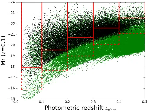
Figure1shows the rest-framer-band absolute magnitudeMr (k-corrected toz =0.1) as a function ofzphotfor galaxies with

r <20.4 in the GAMA fields and for galaxies withr <22.4 in the Stripe 82 area withHerschelcoverage. The red boxes indi-cate the redshift boundaries andMrlimits used to define volume-limited samples. When carrying out the stacking procedure, we further bin galaxies in each redshift slice along theMraxis. The minimum bin width alongMris 0.15 mag but can be increased to

Fig. 1.Rest-framer-band absolute magnitudeMrvs. photometric

red-shiftzphot for DR12 galaxies with r < 20.4 (black dots) and Stripe

82 galaxies withr <22.4 (green dots), in areas withHerschel-SPIRE coverage. For clarity, only 20% of the DR12 sample and 10% of the Stripe 82 sample are plotted. The red boxes indicate the volume-limited subsamples in five redshift slices (solid: DR12; dashed: Stripe 82).

ensure that the minimum number of galaxies in a given redshift andMrbin is 1000.

2.2. Herschel survey 250µm maps

The H-ATLAS survey conducted observations at 100, 160, 250, 350, and 500 µm of the three equatorial fields also observed in the GAMA spectroscopic survey (Driver et al. 2011); these equatorial fields are G09, G12, and G15 centred at a right as-cension of∼9, 12, and 15 h, respectively. For this study, we cut out a rectangle inside each of the GAMA fields with a total area of 95.6 deg2. The version of the data used in this paper is the Phase 1 version 3 internal data release. The SPIRE maps, which have unit of Jy/beam, were made using the methods described by Valiante et al. (in prep.). Large-scale structures and artefacts are removed by running the NEBULISER routine developed by Ir-win (2010). We estimated the local background by fitting a Gaus-sian to the peak of the histogram of pixel values in 30×30 pixel boxes and subtracted this background from the raw map.

As the deeper SDSS Coadd catalogue is located in Stripe 82, we also used maps from the two Herschelsurveys in the Stripe 82 region, i.e. the Herschel Stripe 82 Survey (HerS; Viero et al. 2014) and the HerMES Large-Mode Sur-vey (HeLMS;Oliver et al. 2012). The joint HeRS and HeLMS areal coverage between −10◦ and 37◦ (RA) covers the subset of Stripe 82 that has the lowest level of Galactic dust emission (or cirrus) foregrounds. For this study, we combined 39.1 deg2

in HeRS and 47.6 deg2 _{in HeLMS, which are covered by the}

SDSS Coadd data. The SPIRE data, obtained from theHerschel Science Archive, were reduced using the standard ESA software and the custom-made software package, SMAP (Levenson et al. 2010;Viero et al. 2014). Maps were made using an updated ver-sion of SMAP/SHIM, which is an iterative map-maker designed to optimally separate large-scale noise from signal. Viero et al. (2013) provide greater detail on these maps.

3. Method

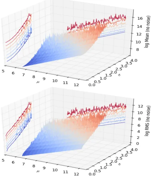
Fig. 2.Top: estimated meanL250 as a function of the intrinsic popu-lation mean (µ) and standard deviation (σ) of logL250. For each set of (µ,σ), we generate∼2000 random numbers representing the 250µm luminosities drawn from the log-normal distribution specified by (µ,σ). The estimates of the mean 250µm luminosity ¯mare derived from these specific realisations of log-normal distributions.Bottom: the estimated standard deviation ofL250 as a function ofµandσ.

dim to be detected at the working wavelength. For a given galaxy sample, we can stack1the 250µm images centred at the positions of the galaxies weighted by luminosity distance squared (D2

L) andkcorrection to derive the mean rest-frame 250µm luminos-ity. To apply thekcorrection at rest-frame 250µm, we used K(z)= νo

νe

!3+β

ehνe/kTdust−1

ehνo/kTdust−1, (1)

whereνo is the observed frequency and νe = (1+z)νo is the

emitted frequency in the rest frame. We assumed a mean dust temperature ofTdust =18.5 K and emissivity indexβ= 2,

fol-lowingBourne et al.(2012).

In this paper, we extend the traditional stacking method to reconstruct the LF. The key assumption is that the rest-frame 250µm luminositiesL250of galaxies in a narrow bin ofzandMr follow a log-normal distribution, i.e. the logarithm of the lumi-nosities, logL250, follow a normal distribution with meanµand

standard deviationσ. In contrast, we used tomdenote the mean of L250andsto denote the standard deviation ofL250. The two

sets of parameters can be related to each other as,

µ=ln (m/p1+s2_/m2_{), σ=} p_{ln (1+s}2_/m2_{). (2)}

With stacking, we can estimate the mean of L250 ( ¯m) and the

standard deviation of L250 ( ¯s). We use mand sto denote the

1 _{We use the IAS library (http://www.ias.u-psud.fr/}

irgalaxies/files/ias_stacking_lib.tgz; Bavouzet et al.

2008;Béthermin et al. 2010) to perform stacking. To avoid introducing bias, we did not clean the image of any detected sources.

Fig. 3.Mean rest-frame 250µm luminosityL250 vs.Mrfor the DR12 (solid squares) and Stripe 82 galaxies (open stars) in five redshift bins. Error bars correspond to the error on the mean.

intrinsic population mean and standard deviation parameters, and ¯mand ¯sto denote estimates2_{of the intrinsic parameters.}

To recover the LF in a given redshift bin, we need to infer µand σas a function of Mr, using combinations of ¯mand ¯s. In Fig.2, we plot the estimated mean and standard deviation of L250, i.e. ¯mand ¯sas a function of the intrinsic population mean

and standard deviation of logL250, i.e.µandσ. To make this plot,

we generated∼2000 random numbers (representing the 250µm luminosities) drawn from a log-normal distribution for each set of (µ,σ) values. The estimates ¯mand ¯swere derived from these specific samples (i.e. realisations) of log-normal distributions. The estimates ¯mand ¯sbecome noisy whenσis large (even in the absence of noise), even thoughmandscan be related toµ andσanalytically (Eq. (2)). This is because ¯mand ¯sare sen-sitive to the large values in the tail of the distribution. To take the effect of realistic noise into account, we injected synthetic galaxies with log-normally distributedL250(drawn from

distri-butions of knownµandσ) at random locations in the map. We can then measure the mean and standard deviation ofL250from

the stacks of synthetic galaxies in the presence of realistic noise and compare with the estimated mean and standard deviation of L250from the stacks of real galaxies. We summarise the main

steps of recovering the 250µm LF using our modified stacking method in Appendix A.

4. Results

Figure3shows the mean rest-frame 250µm luminosityL250as

a function of Mr for the DR 12 and Stripe 82 galaxies. There is good agreement in the overlapping Mrrange; this agreement is generally below 0.1 dex difference. At the faint end, galaxies exhibit a steep correlation betweenL250andMr without signif-icant evolution with redshift. At the bright end, the mean L250

as a function of Mr begins to flatten with significant redshift evolution. As optically red galaxies dominate at the bright end, the redshift evolution can be explained by the evolution in the red galaxy population, which was first observed inBourne et al. (2012). In the two highest redshift bins,z4 andz5, the depth of

2 _{An estimator is a statistic, which is a function of the values in a given}

Fig. 4. 250 µm LF in five redshift bins. Our results are plotted as filled stars (black: Stripe 82; red: GAMA fields), which agree well with previous measurements (green circles:Dye et al. 2010; blue cir-cles: Marchetti et al. 2015). The dashed line is the best fit to our mea-surements (GAMA fields and Stripe 82) and Marchetti et al. (2015).

DR 12 means that we are only able to probe the bright galax-ies with a flattened relation between the meanL250andMr. As explained in Appendix A, our method only works if there is a roughly monotonic relation between the mean L250 and Mr. Therefore, we do not use DR 12 at z > 0.3. Figure 4 shows our reconstructed rest-frame 250 µm LF, using DR 12 in the GAMA fields and the deeper Coadd data in Stripe 82. The lumi-nosity limit reached by our method corresponds to the meanL250

of the galaxies in the faintestMrbin in each redshift slice. Good agreement can be found between our results and previous deter-minations in the overlapping luminosity range. The dashed line in each panel is a modified Schechter function (Saunders et al. 1990) fit to our results (in the GAMA fields and Stripe 82) and measurements from Marchetti et al. (2015),

φ(L)= dn dL =φ

∗L L∗

1−α

exp

"

− 1

2σ2 log 2 10

1+ L L∗

#

, (3)

where φ∗ _{is the characteristic density, L}∗ _{is the}

characteris-tic luminosity, αdescribes the faint-end slope, and σ controls the shape of the cut-off at the bright end. We assume σ and α do not change with redshift. Table 1 lists the best-fit and marginalised error for the parameters in the modified Schechter function. We find strong positive luminosity evolutionL∗₂₅₀(z)∝

(1+z)4.89±1.07and moderate negative density evolutionΦ∗₂₅₀(z)∝

(1+z)−1.02±0.54over 0.02<z<0.5.

5. Conclusion

We study the low-redshift, rest-frame 250µm LF using stacking of deep optically selected galaxies from the SDSS survey on the

Table 1.Best-fit values and marginalised errors of the parameters in the modified Schechter functions.

Parameter Best value Error logL∗

1(z1=[0.02,0.1]) 9.17 0.11

logL∗

2(z2=[0.1,0.2]) 9.37 0.11

logL∗

3(z3=[0.2,0.3]) 9.50 0.12

logL∗

4(z4=[0.3,0.4]) 9.66 0.12

logL∗

5(z5=[0.4,0.5]) 9.87 0.13

logφ∗

1(z1=[0.02,0.1]) –1.60 0.02

logφ∗

2(z2=[0.1,0.2]) –1.60 0.03

logφ∗

3(z3=[0.2,0.3]) –1.70 0.06

logφ∗

4(z4=[0.3,0.4]) –1.59 0.10

logφ∗

5(z5=[0.4,0.5]) –1.92 0.13

σ 0.35 0.01

α 1.03 0.02

Herschel-SPIRE maps of the GAMA fields and the Stripe 82 area. Our method not only recovers the mean 250 µm lumi-nositiesL250of galaxies that are too faint to be individually

de-tected, but also their underlying distribution functions. We find very good agreement with previous measurements. More impor-tantly, our stacking method probes the LF down to much fainter luminosities (∼25 times fainter) than achieved by previous ef-forts. We find strong positive luminosity evolution L∗

250(z) ∝

(1+z)4.89±1.07_{and moderate negative density evolutionΦ}∗

250(z)∝

(1+z)−1.02±0.54_{atz<0.5. Our method bypasses some major}

dif-ficulties in previous studies, however, it critically relies on the input photometric redshift catalogue. Therefore, issues such as photometric redshift bias and accuracy would have an impact. Over the coming years, our stacking method of reconstructing the LF will deliver even more accurate results and also extend to even fainter luminosities and higher redshifts. This is because, although we are probably not going to have any FIR/sub-mm imaging facility that will surpassHerschelin terms of areal cov-erage, sensitivity, and resolution in the near future, our knowl-edge of the optical and near-IR Universe will increase dramati-cally with ongoing and planned surveys such as DES and LSST. In addition, large and deep spectroscopic surveys such as EU-CLID and DESI will further improve the quality of photometric redshift.

Acknowledgements. P.N. acknowledges the support of the Royal Society through

Physics, New Mexico State University, New York University, Ohio State sity, Pennsylvania State University, University of Portsmouth, Princeton Univer-sity, the Spanish Participation Group, University of Tokyo, University of Utah, Vanderbilt University, University of Virginia, University of Washington, and Yale University.

References

Alam, S., Albareti, F. D., Allende Prieto, C., et al. 2015,ApJS, 219, 12

Annis, J., Soares-Santos, M., Strauss, M. A., et al. 2014,ApJ, 794, 120

Bavouzet, N., Dole, H., Le Floc’h, E., et al. 2008,A&A, 479, 83

Beck, R., Dobos, L., Budavári, T., Szalay, A. S., & Csabai, I. 2016,MNRAS, 460, 1371

Béthermin, M., Dole, H., Beelen, A., & Aussel, H. 2010,A&A, 512, A78

Béthermin, M., Le Floc’h, E., Ilbert, O., et al. 2012,A&A, 542, A58

Blanton, M. R., & Roweis, S. 2007,AJ, 133, 734

Bourne, N., Maddox, S. J., Dunne, L., et al. 2012,MNRAS, 421, 3027

Casey, C. M., Berta, S., Béthermin, M., et al. 2012,ApJ, 761, 140

Casey, C. M., Narayanan, D., & Cooray, A. 2014,Phys. Rep., 541, 45

Csabai, I., Dobos, L., Trencséni, M., et al. 2007,Astron. Nachr., 328, 852

Devlin, M. J., Ade, P. A. R., Aretxaga, I., et al. 2009,Nature, 458, 737

Dobos, L., Csabai, I., Yip, C.-W., et al. 2012,MNRAS, 420, 1217

Dole, H., Lagache, G., Puget, J.-L., et al. 2006,A&A, 451, 417

Driver, S. P., Hill, D. T., Kelvin, L. S., et al. 2011,MNRAS, 413, 971

Dye, S., Dunne, L., Eales, S., et al. 2010,A&A, 518, L10

Eales, S., Chapin, E. L., Devlin, M. J., et al. 2009,ApJ, 707, 1779

Eales, S., Dunne, L., Clements, D., et al. 2010a,PASP, 122, 499

Eales, S. A., Raymond, G., Roseboom, I. G., et al. 2010b,A&A, 518, L23

Griffin, M. J., Abergel, A., Abreu, A., et al. 2010,A&A, 518, L3

Hauser, M. G., & Dwek, E. 2001,ARA&A, 39, 249

Lacey, C. G., Baugh, C. M., Frenk, C. S., et al. 2015, MNRAS, submitted [arXiv:1509.08473]

Marchetti, L., Vaccari, M., Franceschini, A., et al. 2016,MNRAS, 456, 1999

Oliver, S. J., Bock, J., Altieri, B., et al. 2012,MNRAS, 424, 1614

Pilbratt, G. L., Riedinger, J. R., Passvogel, T., et al. 2010,A&A, 518, L1

Reis, R. R. R., Soares-Santos, M., Annis, J., et al. 2012,ApJ, 747, 59

Schaye, J., Crain, R. A., Bower, R. G., et al. 2015,MNRAS, 446, 521

Schlegel, D. J., Finkbeiner, D. P., & Davis, M. 1998,ApJ, 500, 525

Symeonidis, M., Vaccari, M., Berta, S., et al. 2013,MNRAS, 431, 2317

Vaccari, M., Marchetti, L., Franceschini, A., et al. 2010,A&A, 518, L20

Appendix A: The modified stacking method

Below we summarise the main steps of recovering the 250µm LF in a given redshift bin using our modified stacking method:

1. Stack the 250µm images centred on the galaxies in a given Mr bin, weighted by luminosity distance squared (D2L) and k-correction. Measure the mean and standard deviation of the rest-frame 250µm luminosityL250, i.e. ¯mand ¯s. Note that

the estimates ¯mand ¯sare affected by instrument noise in the 250µm images.

2. Generaten bootstrap realisations for each sample (i.e. the set of galaxies in a givenMr bin) and repeat Step 1 for all realisations. Form an estimate of the error on ¯mand ¯s, using thenbootstrap realisations.

3. Generate synthetic galaxies3_{with randomL}

250values drawn

from log-normal distributions set by knownµandσvalues and add them to random locations in the map. Theσvalues (i.e. the standard deviation of logLIR) are chosen to sample

linearly between 0.027 and 2.17 with a width of 0.027. The µvalues (i.e. the mean of logLIR) are sampled linearly

be-tween 6.478 and 12.088 with a width of 0.035. Measure the mean and standard deviation ofL250of the synthetic

galax-ies, taking into account the effect of instrument noise in the 250µm images.

4. Repeat Step 3ntimes. Each time sampling different random locations in the maps.

3 _{The number of synthetic galaxies is equal to the number of real}

galax-ies in a givenzandMrbin.

5. By comparing the measured mean and standard deviation of L250of the real galaxies with the mean and standard deviation

estimates of the synthetic galaxies (for allnrepetitions), se-lect all sets ofµandσvalues that give reasonably close mean and standard deviation to the real values usingχ2_statistics.

6. For each set from the accepted µ and σ values, generate log-normally distributed L250and assign them randomly to

galaxies in a given Mr bin. Calculate the resulting distribu-tion funcdistribu-tion ofL250.

7. Repeat Step 6 for all accepted values ofµandσ, so we have multiple realisations of the distribution function of L250for

galaxies in a singleMrbin.

8. Repeat Step 1 to 7 for allMrbins. The 250µm LF is derived by adding up contributions to a givenL250bin from galaxies

in allMrbins. Using the multiple realisations, form a median estimate of the final 250µm LF and its confidence range. For this method to work properly, it is important that the mean r-band luminosity Mr and the mean 250 µm luminosity has a more or less monotonic relation. Otherwise, one could have sit-uations where some sources in a given bin in L250have fainter