A technique based on trade off maps to visualise and analyse relationships between objectives in optimisation problems

(1)

For Peer Review

A Technique Based on Trade-off Maps to Visualise and Analyse

Relationships Between Objectives in Optimisation Problems

Rodrigo Lankaites Pinheiro

ASAP Research Group

School of Computer Science

The University of Nottingham, UK

Dario Landa-Silva

ASAP Research Group

School of Computer Science

The University of Nottingham, UK

Jason Atkin

ASAP Research Group

School of Computer Science

The University of Nottingham, UK

Understanding the relationships between objectives in a multiobjective optimisation problem is important for developing tailored and efficient solving techniques. In particular, when tackling combinatorial optimisation problems with many objectives that arise in real-world logistic scen-arios, better support for the decision maker can be achieved through better understanding of the often complex fitness landscape. This paper makes a contribution in this direction by presenting a technique that allows a visualisation and analysis of the local and global relationships between objectives in optimisation problems with many objectives. The proposed technique uses four steps: first the global pairwise relationships are analysed using the Kendall correlation method; then the ranges of the values found on the given Pareto front are estimated and assessed; next these ranges are used to plot a map using Gray code, similar to Karnaugh maps, that has the ability to high-light the trade-offs between multiple objectives; and finally local relationships are identified using scatter-plots. Experiments are presented for three different combinatorial optimisation problems: multiobjective multidimensional knapsack problem, multiobjective nurse scheduling problem and multiobjective vehicle routing problem with time windows. Results show that the proposed tech-nique helps in the gaining of insights into the problem difficulty arising from the relationships between objectives.

Keywords: multiobjective fitness landscape analysis; trade-off region maps; fitness landscape visualisation; multiobjective combinatorial problems

1 Introduction

The development of solution techniques for multiobjective optimisation problems (MOPs) has wit-nessed many improvements in recent years, partly prompted by real-world applications, but also due to the increasing computational power available; affordable computers are now much more capable of performing the complex computations which are required to solve such problems. Within this field, the study of problems with many-objectives (more than three) calls for special attention: when the number of objectives grows, the number of trade-off solutions may grow exponentially, hence designing algorithms to effectively solve these problems can be very challenging (Fleming et al., 2005; Purshouse

(2)

For Peer Review

and Fleming, 2007). One option to tackle this problem is found in the single-objective problem literat-ure: the design of algorithms that include domain knowledge and are tailored to the specific problem. This approach requires a deeper understanding of the optimisation problem under consideration. In the presence of multiple objectives, it is important to understand the relationships between objectives and the fitness landscape of a given problem. Knowles and Corne (2002) discussed this in the context of the multiobjective quadratic assignment problem, and Castro-Gutierrez et al. (2011) studied the relationships between objectives in the multiobjective vehicle routing problem with time windows.

The multiobjective optimisation literature often focuses on problems in which the multiple object-ives exhibit strongly conflicting natures, as these present an increased challenge for many algorithms, hence being a motivation for applying multiobjective techniques. However, when the number of ob-jectives grows, conflicts could be presented locally rather than globally. Aglobal relationship holds throughout the majority of the search space and is often easy to identify. Alocal relationshipexists in a restricted region of the search space and can be difficult to spot. Understanding local relationships is a useful tool to design tailored algorithms (Garrett and Dasgupta). Additionally, with an increased number of objectives, composite relationships may emerge, i.e. relationships between three or more objectives that occur locally.

It is difficult to assess the multiobjective nature of MOPs and identifying trade-offs is very important for this assessment. However, the existence of multiple objectives may not guarantee the occurrence of trade-offs. Additionally, when tackling multiobjective scenarios, information about trade-offs and relationships between objectives can impact on the choice of solution techniques and algorithmic design – objectives can be grouped or removed, trade-offs can be systematically explored, or the search could be biased towards regions of interest. Additionally, most common benchmark MOPs found in the literature are generated to emulate some sort of behaviour (usually conflicting), hence the fitness landscape is often known beforehand. Examples of this are the ZTD family of functions (Zitzler et al., 2000) and DTLZ test suite (Deb et al., 2002b). However, for real-world optimisation problems, especially combinatorial ones, the fitness landscape is usually unknown and learning its nature may potentially give designers substantial advantages for developing effective specialised algorithms.

Purshouse and Fleming (2003a) discussed some common techniques for analysing and visualising relationships between objectives in MOPs, including scatter plots and parallel coordinates (graphical representations), Kendall correlation (Kendall, 1938) (a quantitative metric), amongst others. Khabza-oui et al. (2004) presented statistical measures. Previous work has also applied some of these techniques to improve the understanding of relationships in specific problems, such as Castro-Gutierrez et al. (2011) who used the Kendall correlation metric to assess the multiobjective vehicle routing problem with time windows and Ishibuchi et al. (2011) who assessed many-objective problems with correlated objectives. However, these techniques are best suited for problems with two objectives and fail to discover insights into problems with a larger number of objectives.

In (Pinheiro et al., 2015), a technique to analyse and visualise relationships (both local and global) between objectives in multiobjective problems was introduced. This technique aims to improve the understanding of the fitness landscape of MOPs by assessing different perspectives of the problem objectives. In the present work, the technique is revisited and is both extended and further investigated, applying it to new problems. In order to be applied, the technique requires an approximation set of non-dominated solutions to be supplied by some means. A novel visualisation tool based on Karnaugh maps (Karnaugh, 1953) is proposed to visualise the relationships between the many objectives. The analysis technique is performed in four steps: first the global pairwise relationships are analysed using the Kendall correlation method; then the ranges of the values found on the given Pareto front are estimated and assessed; next these ranges are used to plot a map using Gray code, similar to Karnaugh maps, that have the ability to highlight the trade-offs between multiple objectives; and finally local relationships are identified using scatter-plots.

It was suggested in (Pinheiro et al., 2015) that the technique could be used to compare the mul-tiobjective natures of different problems and that the information obtained could be used in the design of algorithms. The analysis is extended in this work to two different problems. The technique is first applied to different instances of a multiobjective multidimensional knapsack problem to demonstrate

(3)

For Peer Review

how it can be useful to highlight different multiobjective natures of variations of the same problem. Next, a new set of multiobjective nurse scheduling problem instances is designed, based on the NSPLib (Maenhout and Vanhoucke, 2005) and the technique is applied to show that it can be used to assess the multiobjective aspects of previously unseen instances. The technique is then applied to an existing set of instances of the multiobjective vehicle routing problem with time windows (Castro-Gutierrez et al., 2011), to demonstrate that the technique can help to expand the understanding of that exist-ing dataset. Finally, different problems are compared, to draw conclusions regardexist-ing their common features.

In summary, the contributions of this work are threefold:

1. The usefulness of the analysis technique presented in (Pinheiro et al., 2015) is improved by reducing its reliability on domain knowledge. One weakness of the previous work was the need to define a threshold for the third step of the analysis, because it was exclusively based on domain knowledge or input from the decision-maker. A novel method to calculate better thresholds for the region maps is proposed here, along with a consideration of how to use this information to draw richer conclusions about the multiobjective nature of the given MOP.

2. The technique is shown to facilitate a comparison between the fitness landscapes of different problems, and the usefulness of this information for the crafting of solution algorithms is observed – given two problems with similar fitness landscapes, an efficient solution algorithm for the first problem is more likely to also be efficient for the second one, given that it has similar exploratory capability on both problems.

3. Improved insights on the generation of multiobjective benchmark scenarios are presented. It is shown that in order to generate a MOP benchmark dataset, it may not be sufficient to parametrise constraints to produce scenarios with distinct fitness landscapes. Instead, a combination of parametrised constraints and correlated data is shown to be more effective.

Section 2 surveys related work. Section 3 provides the motivation for this work. Section 4 describes the proposed technique while experimental results applying the proposed technique to three distinct combinatorial problems are presented in Section 6. Finally, Section 7 concludes the paper.

2 Related Work

The topic of analysing fitness landscapes of MOPs is not new to the literature and important progress has been made in the past. Most previous work focuses on adapting single-objective techniques and methods to multiobjective scenarios. Some of the main contributions in this field are outlined here.

Huband et al. (2006) identified the need for properly evaluating MOPs to validate algorithm de-velopment. In their work, they extend the knowledge of several benchmark problems. They assess the problems regarding multiple criteria, including the need for external or medial parameters, the scalable number of parameters and objectives, the problems being dissimilar with regard to para-meter domains and trade-off ranges, the knowledge of the Pareto optima, the optimal geometry, the parameter dependencies, the bias, the mappings and the modality. Although they provide a compre-hensive assessment of the problems studied, the evaluation is specifically useful for the generation of benchmarking scenarios.

Korhonen and Wallenius (2008) surveyed the most common methods used in multiobjective decision-making frameworks, including multivariate statistical methods. They suggest the use of charts and graphs as visual aids in the decision-making process, including bar and line charts to visualise multiple solution vectors. In their work they also raise the importance of developing advanced techniques to further aid the decision-making process. In the same book, Lotov and Miettinen (2008) described techniques for visualising the Pareto optimal set of many-objective problems, including scatterplots and heatmaps.

(4)

For Peer Review

Garrett (2008) and Garrett and Dasgupta adapted single-objective landscape analysis techniques such as analysis of the distribution of Pareto optima, fitness distance correlation, ruggedness, random walk and the geometry of the objective space to obtain insights useful to the tailoring of multiobjective evolutionary algorithms. They apply the proposed techniques to two-objective quadratic and general-ised assignment problems. They conclude that using hybrid algorithms that explore knowledge about the landscape provides performance gains compared to more general approaches.

A graphical approach to evaluate the quality of a Pareto front based on ranks of objectives was proposed by Brownlee and Wright (2012). According to their assessment, the technique may not be suitable for large solution sets as it is based on an individual analysis of solutions.

Verel et al. (2011a) adapted single-objective landscape analysis techniques to set-based multiobject-ive problems with objectmultiobject-ive correlation. Later, Verel et al. (2011b) conducted a study of the landscape of local optima in such problems. Verel et al. (2013) proposed to carry out a priori analysis of a problem by evaluating the problem size, its epistasis, the number of objectives and the correlation values between objectives, to suggest the best way to tackle it. They concluded that, depending on the problem features, different types of algorithms (scalar or Pareto approaches) and sizes of the solution archive should be employed.

Recently, different methods to visualise solutions, such as scatter plots, parallel coordinates and heat maps were reviewed by Walker et al. (2013). They proposed two techniques: a data mining visualisation tool to plot a convex graph, and a new similarity measure of solutions to plot them in a two-dimensional space. Moreover, multiple visualisation techniques for many-objective approxim-ation sets were surveyed by Tusar and Filipic (2015). They also proposed a visualisapproxim-ation method based on orthogonal projections of a section and employed it on four-dimensional approximation sets. Other visualisation techniques include objective wheels, bar graphs and colour stacks, as explored by Anderson and Dror (2001).

Giagkiozis and Fleming (2014) proposed a technique to estimate the Pareto front of continuous optimisation problems, and then used the estimated front to obtain values for the decision variables of interesting solutions. They applied it to convex benchmark problems. The concept involves obtaining an initial solution set (using any multiobjective algorithm) and then calculating a projection matrix of the optimal Pareto set.

Finally, Castro-Gutierrez et al. (2011) assessed the well-known Solomon (Solomon, 1987) dataset of the Multiobjective Vehicle Routing Problem with Time-Windows (MVRPTW) using the objectives pairwise correlation analysis proposed by Purshouse and Fleming (2003a) and concluded that those instances are not suited for multiobjective benchmarking purposes. They then proposed a new set of benchmark instances for the MVRPTW and showed that those instances exhibit an interesting multiobjective nature. These instances are further evaluated in this paper, using the new analysis technique proposed here, showing that the results are consistent with their claim and providing further insights into those datasets.

Therefore, it can be observed that an improved understanding of fitness landscapes of MOPs can help in the development of better solution methods. Additionally, analysis and visualisation of fitness landscapes and relationships in MOPs is a topic of significant interest for researchers. The technique proposed in this paper seeks to make a contribution in this area.

3 Objective Relationships in Multiobjective Optimisation

This research focuses on the investigation of relationships between objectives in MOPs by analysing non-dominated approximation solution sets and their coverage of the objective space. Additionally, the concepts proposed by Purshouse and Fleming (2003a), of conflicting, harmonious and independent objective relationships, are used.

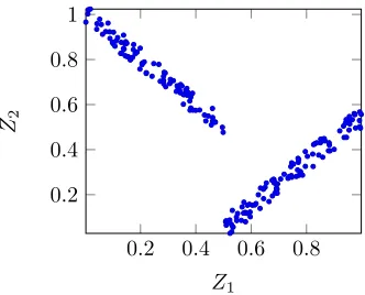
Much of the work in the literature relies on the study of pairwise relationships between objectives (Castro-Gutierrez et al., 2011; Guo et al., 2013; Ishibuchi et al., 2011). However, results obtained solely from this technique can be misleading. Take for instance Figure 1, which shows the scatter plot of two

(5)

For Peer Review

0.2 0.4 0.6 0.8

0.2 0.4 0.6 0.8 1

Z1

[image:5.612.225.391.85.219.2]

Z2

Figure 1: Example of complex relationship between two objectivesZ1andZ2in a 3-objectives optim-isation problem,Z3 is omitted for simplicity.

minimisation objectivesZ1 andZ2 for a scenario with three objectives (Z3is omitted for simplicity). The Kendall correlation value can be calculated as follows: given an approximation solution set and any two objectivesZi andZj wherei=6 j, calculate the number ofconcordant pairsµc anddiscordant pairsµd. A pair of solutions (a, b) is concordant whenZa

i > Z b i and Z

a j > Z

b

j (where Z y

x is the value of objectivexfor solutiony), or whenZa

i < Z b i andZ

a j < Z

b

j. A pair of solutions is discordant when

Za

i > Zib andZja < Zjb, or whenZia < Zib andZja > Zjb. If µis the total number of solutions in the approximation set, then the Kendall correlation coefficientτ can be calculated as follows:

τ= ₁µc−µd 2µ(µ−1)

Considering the global objective space, using techniques such as the Kendall correlation technique, it would be easy to conclude that the objectivesZ1andZ2are independent. However, it is clear that, in fact, the objectives are conflicting whenZ1<0.5 and harmonious whenZ1≥0.5. This misleading loss of information is a consequence of considering the global rather than local objective space, thus identifying onlyglobal relationships between objectives.

(45,68,85),(6,63,99),(34,64,95),

(28,100,48),(98,47,69),(48,62,79),

(72,24,90),(82,79,16),(36,100,97),

(100,87,41),(98,19,87),(85,57,50),

(88,20,73),(91,48,99),(94,31,70),

(56,49,59),(75,93,1),(38,84,85),

(45,78,47)

(a) Non-dominated points.

Z1 -0.30 -0.33

Z2 -0.33

Z3

(b) Scatter-plot matrix and correlation coefficients.

Figure 2: Three-way conflicting objectives

Additionally, common representations fail to highlightcomposite relationships between more than two objectives. Figure 2 shows evidence of that. Figure 2a shows a set of 19 non-dominated points where green values are above 50 and red values are equal to or below 50. It is clear that no point has three values simultaneously above 50. Figure 2b shows the scatter plot and the Kendall correlation

[image:5.612.328.509.470.613.2]

(6)

For Peer Review

coefficients for each pair of objectives. The scatter plot and correlation values do not help to identify the three-way trade-off. Likewise, it is clear that the correlation values do not indicate any strong pairwise correlation.

To better analyse and visualise the multiobjective nature of optimisation problems, techniques are needed that will help in identifying global, local and composite relationships between objectives as well as interesting trade-offs in the fitness landscape.

4 A Four Step Analysis and Visualisation Technique

The analysis technique which was originally proposed in (Pinheiro et al., 2015) is now revisited, refined and enhanced. This is a four-step method to analyse and visualise objectives relationships in MOPs. The following requirements must be met in order to apply the technique:

1. Obtain an approximation to the Pareto optimal set for a subset of instances of the multiobjective problem in hand. This can be obtained by any multiobjective algorithm (MOA), provided that the quality of the solutions is good enough. A combination of different methods is suggested here, to increase the likelihood of obtaining a good quality approximation set. Multiple MOAs are publicly available and frameworks like JMetal (Durillo and Nebro, 2011), ParadiseEO (Cahon et al., 2004) and MOEA Framework (Hadka, 2015) provide efficient implementations of several state of the art algorithms that may be applied to different problem domains.

2. Obtain knowledge of the problem domain and the importance of different objective values. Steps two and three particularly require this, when defining meaningful ranges, quality thresholds and regions of interest.

The aim of the proposed technique is to aid the study of subsets of problem instances, to help the design of more effective tailored algorithms for solving other instances of the same problem. The focus of this work is to investigate the suitability of the technique for that purpose, hence it is applied to three distinct MOPs. Although the need to solve the problem first could be seen as a weakness, there are often similarities between some problem instances, especially for real-world problems, thus insights into one set of instances can give insights into many other instances. Solving many-objective problems is computationally expensive, thus any help in tailoring fast techniques that can provide ‘good-enough’ results is important, and this technique may allow a user to identify similarities between instances which could be exploited. Moreover, the increased understanding of the problem could help to identify strengths and weaknesses in algorithms.

Each step in the analysis brings to light more information regarding any relationships between objectives, the coverage of the feasible region and the trade-off landscapes. The details of the four steps in the proposed technique are presented in the remainder of this section, the results of the analysis of three distinct problems are presented in the next section: a multiobjective multidimensional knapsack problem, a multiobjective nurse scheduling problem and a multiobjective vehicle routing problem with time windows.

4.1 Step 1 – Global Pairwise Relationship Analysis:

The available approximation set of non-dominated solutions is first analysed using Kendall correlation coefficients (Kendall, 1938), to identify global pairwise relationships, as proposed by Purshouse and Fleming (2003a). The existence of strongly conflicting correlations (values< −0.5) immediately in-dicates that a trade-off surface exists. Analogously, the existence of strongly harmonious correlations (values>0.5) indicates that objectives could be aggregated. Objectives identified as independent only prove that the objectives are not globally dependent, but do not imply the absence of local trade-offs in some areas of the fitness landscape.

If independence is detected, the problem could be assessed for the possibility of decomposing the decision variables according to the objectives in order to solve each objective (or groups of objectives)

(7)

For Peer Review

separately, as such an approach has been observed to improve performance (Purshouse and Fleming, 2003b).

4.2 Step 2 – Objective Range Analysis:

Next, the range (the difference between best and worst values observed) of each objective in the approximation set is calculated. The problem domain knowledge or expertise of the decision-maker is then used to assess how to approach each objective; e.g. assign it to a cluster, remove it, etc. This approach assumes that there is some way to categorise solutions into high vs low quality, or acceptable vs unacceptable to the decision-maker. Hence, the availability of a domain-expert or sufficient domain knowledge to determine this, is important.

A meaningful objective is an objective in which the range is large enough such that solutions can be classified into multiple quality categories (good to bad, high to low, acceptable to unacceptable, etc) depending on the problem domain. The existence of this type of objective indicates the presence of a trade-off in the fitness landscape. Analogously, a non-meaningful objective is an objective in which the range is small to the point that its variability can be considered negligible according to the problem domain, thus it is not worth exploring further. Again, the categorisation of solution quality is important, to avoid issues of scaling factors, for example. An objective with a large range of values across the non-dominated solutions, but where all such values are considered by decision-makers to be good (if such is possible), would be a non-meaningful objective. Conversely, even a binary objective where it is important for the objective to have the value of 1 would be meaningful if some of the non-dominated solutions had a value of 0 for the objective.

One way to tackle non-meaningful objectives is to ignore them. With a low enough variability across the approximation set, it is possible that optimising for the other objectives will still result in acceptable values for the non-meaningful objectives. This may be the result of composite relationships or of the characteristics of the data in the scenario. Note that having a small range across the initial solution set does not imply that the range is negligible for the entire objective space. To assess whether this is the case, remove this objective from the MOA, determine a new approximation set, and calculate the ranges of the excluded objective in the new solution set. If the new range is also negligible, then it is likely that the objective can be ignored.

Another option to tackle non-meaningful objectives is to cluster them (Guo et al., 2013). Clustering the objectives will reduce the size of the objective space, but the MOA will still keep some pressure towards optimising these objectives. Arguably the overall results for these objectives may not be as good as solving them separately. However, considering that they all presented small ranges, it is possible that the new solutions will present similar ranges as before.

4.3 Step 3 – Trade-off Regions Analysis:

The third step consists of a quantitative method based on Karnaugh maps (Karnaugh, 1953) to classify the objective space into regions of interest to aid in identifying trade-offs and complex relationships between objectives. A Karnaugh map is a method to visualise and simplify boolean algebra expressions using a truth table. A map fori variables has 2i _{cells. The cells’ labelling follows the Gray code,} therefore any two adjacent cells differ in only one bit. For example, in a three variables scenario, the cells adjacent to cell 0 (0002) are cells 1(0012), 2(0102) and 4(1002). Karnaugh maps are used to group variables because they make it easy to visualise patterns.

Given an approximation set, to build its region map it is necessary to first define, for each objective

Ziwhere (i= 1,2, . . . m), a thresholdti such that values above (assuming a maximisation problem)ti are considered good or acceptable, and values belowtiare considered bad or inadequate. The threshold can be obtained using domain knowledge or empirically – for example, using the average value for each objective as its threshold. Since the threshold value may be important for problems, it can be worth considering alternative values for the threshold, as discussed later.

(8)

For Peer Review

Next, each objective value in each solution is classified as good (✓) or bad (✗) according to the objective’s threshold. For example, a solution (Z1=✓, Z2=✗, Z3 =✓) in a three-objective scenario indicates that forZ1andZ3the objective values are better than their respective thresholds, whileZ2 presents a value which is worse than its threshold.

Aregion map is then drawn. This is similar to a Karnaugh map, but instead of boolean variables, the objectives of the MOP are used. These are arranged such that the cells of the map follow the Gray code (replacing 0’s and 1’s by✓and✗). The map is built with 2m_{regions where each region represents} a single combination of good and/or bad objectives. Each cell in the map represents a regionrk using a binary encoding such that the least significant digit represents objectiveZ1and the most significant digit is objectiveZm. Finally, the region number is identified for each solution (considering✓_{= 0 and} ✗_{= 1) and the number of solutions in each region is determined. The solution of the previous example,}

(Z1=✓, Z2=✗, Z1=✓), falls into regionr2 because 210= 0102. Regionr0represents solutions with good values in all objectives

Z✓

2 Z

✗ 2

Z✓

3 r0 r1 r3 r2

Z✗

3 r4 r5 r7 r6

Z✓ 1 Z ✗ 1 Z ✓ 1 (a) Three Objectives

Z✓

2 Z

✗ 2

r0 r1 r3 r2 Z3✓

Z✓ 4 _r

4 r5 r7 r6

r12 r13 r15 r14 Z ✗ 3

Z✗ 4 _r

8 r9 r11 r10 Z3✓

Z✓ 1 Z ✗ 1 Z ✓ 1 (b) Four Objectives Z✓ 5 Z ✗ 5 Z✓ 2 Z ✗ 2 Z ✓ 2 Z ✗ 2

r0 r1 r3 r2 Z3✓ r16 r17 r19 r18 Z3✓

Z✓

4 _r

4 r5 r7 r6 Z

✓

4 _r

20 r21 r23 r22

r12 r13 r15 r14 Z ✗

3 _r

28 r29 r31 r30 Z ✗ 3

Z✗

4 _r

8 r9 r11 r10 Z3✓

Z✗

4 _r

24 r25 r27 r26 Z3✓

Z✓ 1 Z ✗ 1 Z ✓ 1 Z ✓ 1 Z ✗ 1 Z ✓ 1 (c) Five Objectives

[image:8.612.89.528.246.449.2]

Figure 3: Region map schematics, illustrating the use for 3, 4 or 5 objectives.

Figure 3 shows the region map schematics for 3, 4 and 5 objectives. Each region is labelled according to the Gray code. A shading scheme is used to display the differences between regions, such that regions with lighter tones have a higher number of good objectives than regions with darker tones. The use of these maps makes it easy to spot where solutions are concentrated in the objective space and the existence of trade-offs. When region r0 is not empty, then there exist solutions with good values in all objectives, meaning that the problem could possibly be tackled with single-objective algorithms. Alternatively, that could mean that the threshold could be increased until trade-offs appear. Performing a range analysis in this region could provide further insights into the best approach to take. Conversely, if most solutions fall into regionr2m₋₁, then it is possible that the threshold is set too high and should be lowered for more accurate results. If there are no solutions inr0, but they are scattered throughout the map, then trade-offs have been identified and the map can be used to visualise them.

Threshold Analysis

As previously mentioned, moving the threshold for objectives may sometimes help to clarify and further investigate the trade-offs. Region maps from modified threshold values can be used to determine additional information about the multiobjective nature of the problem, including:

• The maximum threshold such that all solutions are considered good in all objectives. This

(9)

For Peer Review

(10)

For Peer Review

multiple instances of a problem present consistent landscapes, then the information obtained and the algorithmic designed could be more likely to succeed in solving other previously unseen instances of the problem.

The following sections present experimental results from applying the proposed analysis and visu-alisation technique to three distinct MOPs: a multiobjective multidimensional knapsack problem, a multiobjective nurse scheduling problem and a multiobjective vehicle routing with time windows. All of the steps for the proposed analysis are performed for each of the datasets for each problem and the new knowledge obtained from doing so is discussed.

5 Problem Scenarios

In order to illustrate the analysis technique and provide a comparison between different problems, it has been applied to different multiobjective combinatorial problems. This will illustrate different benefits and insights from the technique.

5.1 Multiobjective Multidimensional Knapsack Problem (MOMKP)

In the multiobjective multidimensional knapsack problem (Lust and Teghem, 2010), there aren items (i= 1, . . . , n) withm weightswi

j (j= 1, . . . , m) andp profitscik (k= 1, . . . , p). The aim is to select a set of items to maximise thepprofits while not exceeding the capacitiesWj of the knapsack. Decision variablexi indicates if item iis selected (xi = 1) or not (xi = 0). This problem can be formulated as follows:

maximise n

X

i=1

ci

kxi k= 1, . . . , p

subject to n

X

i=1

wi

jxi ≤Wj j= 1, . . . , m

xi∈0,1 i= 1, . . . , n

Five MMKP datasets are considered here, each of which has five instances, all withm= 4,p= 4,

n= 1000 and Wj= 50000. The first four datasets were generated following the guidelines in Bazgan et al. (2007) and are as follows:

• Set A: Independent random instances wherewi

j∈N [1,1000] andcik ∈N [1,1000].

• Set B: Uncorrelated harmonious instances where

wi

j ∈N [1,1000], ci1 ∈N [1,1000] and cik ∈N [max {cik−1 −100,1} , min{cik−1+ 100,1000}] for

k= (2,3,4).

• Set C: Uncorrelated conflicting instances where wi

j ∈N [1,1000], ci1 ∈N [1,1000] and cik ∈N [max{900−ci

k−1,1}, min{1100−c i

k−1,1000}] fork= (2,3,4).

• Set D: Correlated conflicting instances wherewi

1∈N [max{900− |ci1−c4i|,1},min{1100− |ci1−

ci

4|,1000}],wij∈N [max{900− |cik−c i

k−1|,1},min{1100− |cik−c i

k−1|,1000}],ci1∈N [1,1000] and

ci

k ∈N [max{900−cik−1,1},min{1100−cik−1,1000}] fork= (2,3,4).

(11)

For Peer Review

• Set X: Correlated special set where:

ri_∈ R[0,1]

ci k



      

      

ci

1∈N [900,1000], ci2∈N [ci1,1000], cik∈N [0,100] fork= (3,4). ifri≤0.1

ci

3∈N [900,1000], ci4∈N [c31,1000], cki ∈N [0,100] fork= (1,2). if 0.1< ri≤0.2

ci

1∈N [900,1000], ci3∈N [c11,1000], cki ∈N [0,100] fork= (2,4). if 0.2< ri≤0.3

ci

2, ci3∈N [900,1000] andci1, ci4∈N [0,100]. if 0.3< ri≤0.4

ci

k∈N [0,1000]. ifri>0.4

wi

1=ci1+ci2+ci3

w2i =c i 2+c

i 3+c

i 4

wi

3=ci1+ci3+ci4

w4i =c i 1+c

i 2+c

i 4

SetAcontains only independent objectives. In setBall objectives are harmonious. SetCcontains three pairs of conflicting objectives, (Z2, Z1), (Z3, Z2) and (Z3, Z4), while the weights are uncorrelated. SetDhas conflicting objectives, like setC, but the weights are correlated to the objective values. The fifth setX was tailored to provide a misleading scenario.

5.2 Multiobjective Nurse Scheduling Problem (MONSP)

An extension of the nurse scheduling problem (NSP) presented by Maenhout and Vanhoucke (2007) is also considered. The original problem consists of creating a work plan for a set of nurses, that must be assigned shifts across a time period (week or month) to cover hospital requirements. The problem is composed of a number of hard and soft constraints to be considered when generating each individual schedule. The hard constraints define strict work regulations and the soft constraints define working policies and desirable aspects. For this work the number of objectives is artificially extended using preferences and soft constraint violations as additional objectives.

• Hard Constraints: The NSP has two hard constraints, both of which aim to avoid certain shift patterns. The first forbids the assignment of an afternoon shift before a morning shift. The second forbids the assignment of a night shift before a morning or an afternoon shift.

• Soft Constraints: There are four soft constraints that represent nurses’ preferences. The first defines a minimum and maximum number of working days within the scheduling period. The second defines a minimum and maximum number of consecutive working assignments. The third defines a minimum and maximum number of assignments of each shift type in the scheduling period. The fourth soft constraint defines a minimum and maximum number of consecutive shift assignments of the same type.

• Preferences: The preferences represent the main objectives for the MONSP. Each preference is a numerical value relating to a nurse and a shift. It could represent the nurse preference regarding that shift, the hospital preference to assign that nurse to that shift, the patients’ preferences, or a combination of these.

The MONSP can be defined as follows. Given a set N of nurses, whereN ={n1, n2, . . . , n|N|}, a setD of days whereD ={d1, d2, . . . , d|D|} and a setS of shifts whereS ={s1, s2, . . . , s|S|}, find an assignment of shifts for each daydi ∈ D, such that each nurse nj ∈ N has been assigned a specific shiftsk ∈S and hard constraints are met. Shifts refer to either a given working period (early, day or night shift) or a rest period (free shift). Each tuple (nurse,day,shift) has a set ofmvalues representing different preferences regarding that nurse being assigned to that shift on that day. The different preferences may represent personal preferences, the hospital preferences, patient preferences, costs,

(12)

For Peer Review

[image:12.612.127.483.140.386.2]

etc. The (multiple) objectives to optimise consist of the sum of each type of preference value, and the sum of a set of soft constraints.

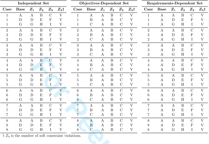
Table 1: Generational patterns for the MONSP using the NSPLib files. Letters represent base files.

Independent Set Objectives-Dependent Set Requirements-Dependent Set Case Base Z1 Z2 Z3 Z4† Case Base Z1 Z2 Z3 Z4† Case Base Z1 Z2 Z3 Z4†

1 A A B C V 1 A A B C V 1 A A B C V

1 D D E F V 1 B A B C V 1 A D E F V

1 G G H I V 1 C A B C V 1 A G H I V

†Z4is the number of soft constraint violations.

NSPLib is a library with problem instances for the NSP (Maenhout and Vanhoucke, 2005). Two types of files are present: base files, which describe the preferences, and case files which specify the constraints. The data from that library was used in this work, with the addition of extra base files to represent the new preference values. Four objectives are considered, so each instance is composed of the existing case file and base file, plus three new objective files. Table 1 presents the details for the different sets, where A to I are different base files (different preference values),Z1 to Z3 are the new preference objective values andZ4 is the count of soft constraint violations.

• Independent Set (IS): There is no correlation between base file and objectives files (all ob-jective files are distinct). The aim is that the fitness landscape will be different for different instances.

• Objective-Dependent Set (ODS): This set uses the same objectives files for all instances, but the base files change. This set assess whether keeping the objectives information across all instances will generate a standardised fitness landscape.

• Requirements-Dependent Set (RDS):This set employs a common base file for all instances but defines different objectives files for each instance. The goal of this scenario is to assess whether keeping a problem base and changing the objectives information has an impact on the fitness landscape of the instances in this set.

Weekly problems with 25, 50 and 100 nurses were generated using random base and objective files following the generational pattern presented. Hence, each set considered in this work is constituted of 75 instances totalling 225 problem instances.

(13)

For Peer Review

5.3 Multiobjective Vehicle Routing Problem with Time Windows

(MOVRPTW)

A Multiobjective Vehicle Routing Problem with Time Windows (MOVRPTW) is defined on a graph

G= (V, E) whereV is the set of vertices representing the depot (vertex 0) and the customers (vertices 1. . . n) where each customer has a demand pi (i = 1, . . . , n). The depot has h identical vehicles available, with capacityQthat must satisfy all demands from all customers. The edge setE denotes all possible connections between all vertices. Each edge (from vertex i to vertex j) has a cost that represents the distance or time, denoted bycij. Each customer must be served during a time window [aij, bij]. If a vehicle arrives early, it must wait until the beginning of the time window. Once the vehicle arrives at the customer, it stays there until the delivery is completed, for a duration known as the service times.

Castro-Gutierrez et al. (2011) proposed a benchmark set for the MOVRPTW. They consider five objectives: number of vehicles (Z1), total travel distance (Z2), makespan (Z3), total waiting time (in case of early arrival) (Z4), and total delay time (Z5). They designed their instances based on different characteristics of the problem and each instance is a combination of these features. The features that constitute an instance are:

• Number of customers: 50, 150 and 250 customers.

• Time window: five different profiles {tw0,tw1,tw2,tw3,tw4} of time windows across eight hours were used. These are defined below in terms of minutes from the start of the working day 0 = 8:00am, 480 = 4:00pm, etc.). Customers are randomly assigned to one time-window:

– tw0: [0,480].

– tw1: [0,160],[160,320],[320,480]. – tw2: [0,130],[175,305],[350,480]. – tw3: [0,100],[190,290],[350,480].

– tw4: all time-windows fromtw0, tw1, tw2 andtw3.

• Demand types: three values for the demandare used{10, 20, 30}, uniformly distributed.

• Vehicle capacity: the capacity of the vehicles are calculated according to aδ parameter such that Q=D+δ/100(D−D), whereD = max

(i=1,...,n)pi and D =

Pn

i=1pi. The dataset considers threeδvalues (δ0 = 60,δ1 = 20,δ2 = 5).

• Service time: three values of service time{10, 20, 30}are used, uniformly distributed. In total, there are 45 instances, and these are publicly available1.

6 Application of the Proposed Technique

To obtain the approximation sets, the MOEA/D (Zhang and Li, 2007) and NSGA-II (Deb et al., 2002a) algorithms were chosen. Initial experiments showed that both algorithms struggled to produce good approximation sets due to the difficulty of tackling many-objective problems, hence to improve the obtained Pareto fronts the following mechanism was applied to all datasets: for each instance, a single-objective genetic algorithm was executed for each single-objective alone, then both NSGA-II and MOEA/D algorithms were executed on each pair and triplet of objectives. All of the non-dominated solutions obtained were then combined into a single archive which was used to initialise further executions of the algorithms: Three runs of MOEA/D and three runs of NSGA-II were then executed, considering all objectives, where half of the individuals for the initial population were randomly drawn from the

1

https://github.com/psxjpc/ – Acessed: 2016-09-22

(14)

For Peer Review

archive and the other half were randomly generated. The final approximation set was formed from all of the non-dominated solutions which were found in the process. Both NSGA-II and MOEA/D used a population of 200 individuals, binary tournament selection and half uniform crossover (Eshelman, 1990) for 1.5×106 _{function evaluations each run.}

6.1 Multiobjective Multidimensional Knapsack Problem

Using the process described above, non-dominated sets were obtained, with approximately 900 com-bined solutions for each instance in setA, 3 for each instance in setB, 550 for each instance in setC, 1500 for each instance in setD and 2500 combined solutions for each instance in setX. Only a few non-dominated solutions were found for instances in set B because the objectives there are strongly harmonious. Therefore, when maximising one of the objectives, the other objectives are also maxim-ised, resulting in insufficient data for some of the analysis steps. However, the results are presented for completeness and illustrate that the number of solutions obtained can have a major impact on the analysis, and that it is important to have a comprehensive set, with enough well-spread solutions.

Z1− Z2

Z1− Z3

Z1− Z4

Z2− Z3

Z2− Z4

Z3− Z4 −1

−0.5 0 0.5 1

Set A Set C Set D Set X

Figure 5: Pairwise correlations for each set of instances.

Step 1 - Global Pairwise Relationships Analysis. The results of this step are in Figure 5. Note that coefficient values for setB are not provided for the reason given above. The figure presents the individual pairwise correlation value for each combination of objectives. As expected for fully independent objectives, setAhas values close to 0. The values for setsC andD are also predictably close to either 1 or −1 indicating global conflicting or harmonious relationships. Set X has values similar toA– they do not reveal a strong global relationship between objectives as they are closer to 0 than to 1 or−1. Also, in set X it is not possible to decompose the decision variables according to the objectives, as every item has all weights and values above zero.

Step 2 - Objective Range Analysis. The results for this step are in Figure 6. The x axis presents the sets grouped by objective. Theyaxis presents the minimum, maximum and average value of each objective as a percentage of the overall maximum value found for the respective objective Considering setB, it can be seen, that the set presents small ranges of less than 0.3% on average. In this dataset, all objectives are harmonious and the solutions found are all located in a small region of the objective space. These few solutions dominated all other solutions explored. Both setsC and D

present similar results to each other with large ranges for each objective (over 60%). This is expected since these are instances with conflicting objectives and present global trade-offs. The large ranges mean that while there are solutions with good values for a given objective, at least one other objective has a poor value.

While the global pairwise relationship analysis (step 1) hinted that setsAandX were similar, the difference between them now becomes clear with the results from step 2. In setA, each objective range

(15)

For Peer Review

(16)

For Peer Review

Z✓ 2 Z ✗ 2 Z✓ 4

0.0% 0.3% 0.9% 0.1% Z✓

3

0.5% 5.3% 17.1% 4.6%

Z✗ 3 Z✗

4

8.7% 7.4% 13.8% 11.6%

4.4% 8.5% 10.5% 6.5% Z✓

3 Z✓ 1 Z ✗ 1 Z ✓ 1

(a) Overall distribution of solutions.

Z✓ 2 Z ✗ 2 Z✓ 4

0% 20% 80% 20% Z✓

3

40% 100% 100% 100%

Z✗ 3 Z✗

4

100% 100% 100% 100%

80% 100% 100% 100% Z✓

3 Z✓ 1 Z ✗ 1 Z ✓ 1

[image:16.612.125.487.83.186.2]

(b) Frequency of instances.

Figure 8: Results for the trade-off regions analysis for Set A.

The range threshold was set to the minimum value such that there are no solutions inr0.

In addition to the distribution of solutions map, the frequency of instances region map is also introduced here, displaying the percentage of instances that contain at least one solution in a region. A value of 100% in a region means that in all instances at least one solution can be found in that region. In setA(Figure 8) the front is well distributed. Solutions can be found in all regions, scattered throughout the objective space, as a result of the independent objectives.

Z✓ 2 Z ✗ 2 Z✓ 4

0.0% 0.0% 0.0% 0.0% Z✓

3

0.0% 20.6% 2.9% 10.6%

Z✗ 3 Z✗

4

0.0% 8.7% 6.6% 6.2%

0.0% 13.3% 8.2% 22.9% Z✓

3 Z✓ 1 Z ✗ 1 Z ✓ 1

Z✓ 2 Z ✗ 2 Z✓ 4

0% 0% 0% 0% Z✓

3

0% 100% 100% 100%

Z✗ 3 Z✗

4

0% 100% 100% 100%

0% 100% 100% 100% Z✓

3 Z✓ 1 Z ✗ 1 Z ✓ 1

Figure 9: Results for the trade-off regions analysis for Set C.

Z✓ 2 Z ✗ 2 Z✓ 4

0.0% 0.0% 0.0% 0.0% Z✓ 3

0.0% 54.1% 3.6% 5.5%

Z✗ 3 Z✗

4

0.0% 6.1% 11.0% 2.0% 0.0% 5.8% 2.0% 10.0% Z✓

3 Z✓

1 Z

✗

1 Z1✓

Z✓ 2 Z ✗ 2 Z✓ 4

0% 0% 0% 0% Z✓

3

0% 100% 100% 100%

Z✗ 3 Z✗

4

0% 100% 100% 100%

0% 100% 100% 100% Z✓

3 Z✓ 1 Z ✗ 1 Z ✓ 1

Figure 10: Results for the trade-off regions analysis for Set D.

The global relationships are clear for setsC (Figure 9) andD (Figure 10). There are no solutions with good values in all objectives and most instances present no solution with good values in three of the objectives. The majority of the solutions are situated whereZ1 and Z3 alone have good values or whereZ2 and Z4 alone have good values, as these are the harmonious pairs. Additionally, it can be observed that almost no solutions are present in conflicting areas. For instance, whereZ1 and Z2 present good values simultaneously. Moreover, solutions in conflicting areas should be close to the chosen threshold.

The set X (Figure 11) does not contain solutions in r0 and there are no solutions in regions r1,

r2,r4 andr8, meaning that no good values can be simultaneously found for three or more objectives.

[image:16.612.121.487.306.571.2]

(17)

For Peer Review

(18)

For Peer Review

The trade-off regions are clear for sets C and D. There is also a noticeable gap in the objective space whenZ1 is in the range from 0 to 0.5 and when the remaining objectives are in the range from 0 to 0.4, approximately. Moreover, the landscape of the objective space appears to be similar for all instances of each of the setsC andD.

Since the data was uniformly generated, these gaps are unlikely to arise from the data itself, and could represent limitations in the solution algorithms, indicating that they did not explore the entire front. It is well known that the performance of some MOEAs is limited when the number of objectives is more than three (Giagkiozis and Fleming, 2012).

SetX presents a unique scenario and patterns and gaps can be identified in the objective space. There is a lack of solutions with values within [0.85,1]. This is again likely to be due to limitations of the solution algorithms. However, it can be seen that the size of the gap is small, confirming that instances with strongly conflicting objectives present a bigger challenge for these algorithms. Several local relationships can also be identified. WhenZ1ranges from 0.5 to 0.8, the three remaining objectives simultaneously conflict and harmonise. Knowing that only two simultaneous objectives present high values (from the region map analysis), it can be concluded that wheneverZ1increases, only one of the other objectives simultaneously increases too.

6.1.1 Discussion

The proposed analysis and visualisation technique can aid in understanding the multiobjective nature of the problem instances considered. Looking at only the correlation coefficients, it could be concluded that: setsAandX do not present interesting multiobjective traits, that setB is inconclusive and that setsC and D present conflicting and harmonious objectives. However, by applying this analysis and visualisation technique, a more comprehensive understanding of these instance sets can be gained.

As fully random instances, datasetAdoes not present relevant global or local pairwise relationships according to the global pairwise analysis (step 1) and the multiobjective scatter plot analysis (step 4). Additionally, the objective range analysis (step 2) shows that even though there is a large set of non-dominated solutions, these are concentrated in a reasonably small area of the search space. For this dataset, the information from the trade-off region maps can be used to interact with the decision-maker to identify which regions are of more interest and then use single-objective optimisation algorithms to find solutions in that region. Since there are solutions in all of the regions of the map, any objective vector could provide an adequate solution.

SetBpresents a completely harmonious case and by analysing the ranges and bearing in mind that the algorithms found just a handful of solutions, it can be concluded that a single-objective algorithm aiming to maximise any of the objectives could provide a good solution.

Sets C and D present similar scenarios, hence the correlation between weights and coefficients does not impact on the nature of the problem. The entire solution set represents a huge trade-off. The algorithms were not successful in expanding along the front and they mainly explored the region surrounding the intersection of the trade-off. Nonetheless, by perceiving that all instances in these sets have similar landscapes and by knowing the approximate boundaries of each objective (by applying single-objective algorithms to each objective alone), the landscape of solutions could be estimated for other instances in those sets. The search could then be directed to the regions of interest after presenting the expected trade-offs to the decision-maker. However, if it is imperative to use an a posteriori approach, the global pairwise analysis and the scatter plots provide sufficient information to make feasible the grouping of harmonious objectives.

Finally, set X presents a quite different picture. By only evaluating the global pairwise analysis (step 1) it could be concluded that there is no strong pairwise relationship between objectives. How-ever, the objectives range analysis (step 2) shows that in fact there are non-dominated solutions that vary greatly in quality. This is an indication of the existence of trade-offs (as can be seen by comparing this set with sets C and D). The trade-off region analysis (step 3) showed the existence of overall trade-offs as it is not possible to have solutions with good values in more than two objectives simultan-eously. Finally, the multiobjective scatter plot analysis (step 4) identified local relationships between

(19)

For Peer Review

objectives and gaps in the objective space, pointing to the existence of local conflicts. Therefore, in-stances in datasetX exhibit a distinctive multiobjective nature perhaps with interesting options for a decision-maker. A sound possibility to tackle this problem would be to use the region map to identify the regions of interest and then locate those regions in the scatter plot. In cases where a selected region contains a local conflict, the algorithm proposed by (Knowles and Corne, 2002) could be used to reach the trade-off front and then expand through it.

6.2 Multiobjective Nurse Scheduling Problem

To assess the MONSP, the instances were initially grouped into the three sets described above: IS, ODS and RDS. However, meaningful dissimilarities were not obvious between the sets, because they presented similar fitness landscapes, meaning that the process to generate the instances did not create sufficiently different scenarios. However, after evaluating the data, a different grouping of instances was identified according to case files:

• Set A:Instances built using the case files 1, 2, 3, 4 and 6.

• Set B:Instances built using the case files 5, 7 and 8.

Z1− Z2

Z1− Z3

Z1− Z4

Z2− Z3

Z2− Z4

Z3− Z4 −1

−0.5 0 0.5 1

IS ODS RDS Cases A Cases B

Figure 13: Pairwise correlations for each set of instances.

The results of the analysis for these new sets A and B are presented here, along with the results for the original sets (IS, ODS and RDS) to validate the claim regarding their similarities.

Step 1 - Global Pairwise Relationships Analysis. Figure 13 presents the results for the pairwise relationships analysis. Note that all solid lines representing the generated sets have similar values on all pairs of objectives. Now it is visible that set B approximately follows the curve of the generational sets, however, set A slightly diverges for (Z1−Z3), (Z1−Z4) and (Z2−Z3). Nonetheless, it is clear that the differences are minimal and that no set presents strong global pairwise relationships. Step 2 - Objective Range Analysis. In the objective range analysis the differences between the generated sets and the new sets A and B becomes evident. Figure 14a compares the ranges between the generated sets. Thexaxis presents the sets grouped by objective. They axis presents the minimum, maximum and average value of each objective as a percentage of the overall maximum value found for the respective objective. The similarity across all sets in the ranges and average values for all objectives is apparent. However, Figure 14b shows that although the average values and ranges are equivalent between sets A and B on Z1, Z2 and Z3, the maximum and minimum values found for set A are roughly 10% lower than for set B. Additionally, for objective Z4 both ranges and average values are noticeably smaller for set A. It can be concluded that grouping the instances based on the generated sets did not present any meaningful differences. However, considering the new sets A and B,

(20)

For Peer Review

Z1 Z2 Z3 Z4

0% 20% 40% 60% 80% 100% P er ce n tage of th e m ax im u m val u e IS ODS RDS

(a) Generational sets.

Z1 Z2 Z3 Z4

0% 20% 40% 60% 80% 100% A B

[image:20.612.119.499.85.247.2]

(b) Distinct cases.

Figure 14: Range analysis results for both the generational sets and the distinct cases. In each line, the central point is the average value for the set, with the top and bottom of the line representing the maximum and minimum values found, respectively.

0 0.2 0.4 0.6 0.8 1

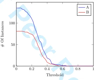
[image:20.612.223.390.300.438.2]

0 50 100 Threshold # O f In st an ce s A B

Figure 15: Threshold analysis showing the number of scenarios with solutions found in regionr0when the threshold decreases.

meaningful differences are apparent. Therefore, from this point on, the analysis considers these case sets.

Step 3 - Trade-Off Region Analysis. The results of the trade-off region analysis for sets A and B are now presented. The threshold analysis is shown in Figure 15, where both curves can be seen to be similar and to converge to roughly the same point, showing that in both cases no solution inr0can be found with more than 60% of the maximum values. This means that to obtain an objective with more than 60% quality, at least one other objective will present an inferior value.

Z✓ 2 Z ✗ 2 Z✓ 4

0.0% 5.6% 8.1% 5.1% Z✓

3

4.1% 6.7% 20.6% 8.4%

Z✗

3 Z✗

4

2.8% 0.3% 0.0% 1.5%

16.4% 4.8% 8.2% 7.5% Z✓

3 Z✓

1 Z

✗

1 Z1✓ (a) Overall Distribution of Solu-tions. Z✓ 2 Z ✗ 2 Z✓ 4

0.0% 63.7% 80.0% 65.9% Z✓

3

63.7% 78.5% 86.7% 88.9%

Z✗

3 Z✗

4

23.7% 9.6% 1.5% 18.5%

91.1% 67.4% 70.4% 68.9% Z✓

3 Z✓ 1 Z ✗ 1 Z ✓ 1

Figure 16: Region maps for Cases A.

[image:20.612.161.449.582.677.2]

(21)

For Peer Review

The region maps for sets A and B are shown in Figures 16 and 17. Sets A and B are similar regarding the regions where solutions can be found, but some differences can be observed. The first difference is that the frequency of solutions is higher in most regions for set B, meaning that the fitness landscapes of instances in B are more alike than the instances in A. In both cases, solutions can be found in all regions of the map, as for the MOMKP independent set (Figure 8). The difference, however, is that in the independent MOMKP set, there were 100% frequencies in most regions while here the values vary greatly. This means that the instances share less in common between themselves than in the independent MOMKP case.

Z✓

2 Z

✗

2

Z✓

4

0.0% 4.5% 6.3% 5.5% Z✓

3

4.2% 3.7% 7.8% 4.7%

Z✗

3 Z✗

4

5.3% 0.7% 0.1% 1.4%

37.1% 7.2% 2.6% 8.7% Z✓

3 Z✓

1 Z

✗

1 Z1✓ (a) Overall Distribution of Solu-tions.

Z✓

2 Z

✗

2

Z✓

4

0.0% 76.5% 92.6% 74.1% Z✓

3

85.2% 92.6% 96.3% 97.5%

Z✗

3 Z✗

4

81.5% 35.8% 7.4% 50.6%

98.8% 87.7% 65.4% 91.4% Z✓

3 Z✓

1 Z

✗

1 Z

✓

1

Figure 17: Region maps for Cases B.

Step 4 - Multiobjective Scatter Plot Analysis. Finally, Figure 18 presents the scatter plot graphs of all individual cases (18a–18h), for set A (18i) and for set B (18j). The Pareto front looks similar in each case, with only minor differences, which are highlighted for sets A and B. A higher concentration of solutions with lowZ3 values when Z1 /0.2 can be observed for set B than for set A, along with a higher concentration of largeZ4 values for the same interval. However, there are no clear trade-off regions and the overall appearance of both sets is closer to the independent MOMKP set than to a scenario where global and local relationships and trade-offs are evident.

6.2.1 Discussion

The NSPLib is a relatively well-known single-objective NSP problem database, that was used here to generate scenarios for the MONSP. A straightforward process to create different sets of instances was followed here, maintaining either the objectives information or the base problem definition across all instances. Then, the proposed analysis technique was applied to assess whether these new instances present significant multiobjective traits or not.

The initial two steps of the analysis revealed that the generated sets do not present meaningful differences between themselves. Hence, by grouping the instances using objective files or base file, generates no dissimilarities in fitness landscapes across different instances. The reason for that be-haviour is that the data is based on a uniform distribution, hence there are no patterns that could result in different landscapes. When grouping the instances by the case files (which describes the soft constraints), slight dissimilarities were noted between two sets, A and B, namely inZ4 ranges, which presented much smaller values for set A.

Additionally, the fairly high ranges presented in step two showed that it is not possible to have near-optimal values in all objectives simultaneously. However, the threshold analysis and the region maps showed that the distribution of solutions is well spread throughout the Pareto front, meaning that solutions can be found in all regions of the solution space and hence the decision maker can decide about the desired quality of each individual objective. Finally, the scatter plot analysis resulted in graphs resembling the independent MOMKP set, with little difference between sets A and B.

It is then concluded that due to the uniform distribution of the data of the NSPLib, the generated sets did not pose any relevant multiobjective difference between themselves. However, some distinct features were found due to different constraint set ups, a scenario which is completely different from that of the MOMKP instances, where all of the differences were due to the data itself while the constraints remained unchanged. What the instances of set B (cases 5, 7 and 8) have in common is

(22)

For Peer Review

(23)

For Peer Review

6.3 Multiobjective Vehicle Routing Problem with Time Windows

Castro-Gutierrez et al. (2011) proposed a new set of benchmark instances for the MOVRPTW after identifying that some instances provided in the literature do not present an interesting multiobjective benchmarking scenario. They proposed different sets based on different time windows (tw0, . . . , tw4) and capacity definitions (δ0, δ1, δ2). These are now considered using the proposed analysis tech-nique, to assess whether changing time windows and capacities impacts on the fitness landscape of the MOVRPTW.

[image:23.612.161.463.255.459.2]

Step 1 - Global Pairwise Relationships Analysis. The global pairwise relationship analysis (Figure 19) corroborates the claim that these instances provide interesting multiobjective challenges, as some pairs of objectives have either high harmonious or conflicting relationships. It is, however, notice-able that changing the time windows andδdoes not greatly impact on the nature of the pairwise global relationships. The only exception is withtw0 which slightly deviates from the other configurations by presenting stronger (conflicting and harmonious) relationships.

Z1− Z2

Z1− Z3

Z1− Z4

Z1− Z5

Z2− Z3

Z2− Z4

Z2− Z5

Z3− Z4

Z3− Z5

Z4− Z5

−1

−0.5 0 0.5 1

tw0 tw1

tw2 tw3

tw4 δ0

δ1 δ2

Figure 19: Pairwise correlation values (yaxis) for each pair of objectives (xaxis). The results for each set of instances are shown in a different colour.

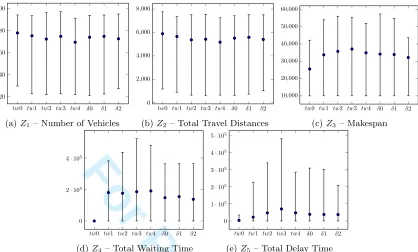
Step 2 - Objective Range Analysis. On the objective range analysis (Figure 20), because the values of individual objectives are similar, the actual values are presented here rather than the relative margin, with a chart for each objective. Excluding Z4 and Z5 for tw0, all objectives present high ranges, again supporting the claim of interesting multiobjective scenarios. The average values found for all setups are similar, but some ranges, namelyZ4 andZ5 present high variance. OnZ4 andZ5, it is clear thattw0 is smaller than the other scenarios. Z5 (20e) is also the objective with the larger discrepancy between sets.

Step 3 - Trade-Off Regions Analysis. The threshold analysis, presented in Figure 21, reveals that there are no instances with solutions inr0 when the threshold is roughly 60% or higher, meaning that if a solution with over 60% quality in at least one criterion is required, then one or more different criteria will present inferior quality. The steepness of the chart is also accentuated if compared to the MONSP, meaning that the instances in the MOVRPTW are more alike than the MONSP instances.

Figure 22 presents the region map and the frequency map using the threshold found. Many regions without solutions are identified, representing trade-offs for the decision-maker. Some global relation-ships can also be observed, for instance, becauseZ1andZ2are harmonious, few solutions can be found whenZ1=✓ andZ2=✗and vice-versa.

Interestingly, because Z3 and Z5 are fairly globally harmonious, a relationship similar to Z1 and

(24)

For Peer Review

tw0 tw1 tw2 tw3 tw4 δ0 δ1 δ2

20 40 60 80 100

(a)Z1 – Number of Vehicles

0 2,000 4,000 6,000 8,000

(b)Z2– Total Travel Distances

10,000 20,000 30,000 40,000 50,000 60,000

(c)Z3 – Makespan

0 2·105

4·105

(d)Z4 – Total Waiting Time

0 1·105

2·105

3·105

4·105

5·105

[image:24.612.99.517.82.334.2]

(e)Z5 – Total Delay Time

Figure 20: Range analysis results for each objective considering instances with different time windows and delta set-ups. In each line, the central point is the average value for the set, with the top and bottom of the line representing the maximum and minimum values found, respectively.

0 0.2 0.4 0.6 0.8 1

0 10 20 30 40

Threshold

#

O

f

In

st

an

ce

s

Figure 21: Threshold analysis showing the number of scenarios with solutions found in regionr0when the threshold decreases.

Z2would be expected, however over 17% solutions are in regions whereZ3=✓andZ5=✗orZ3=✗ andZ5=✓.

Step 4 - Multiobjective Scatter Plot Analysis. Figure 23 presents the scatter plots of all sets and the combined overall scatter plot. The first relevant information shown is that the number of solutions fortw0 is noticeably smaller than for the other time windows. This happens because each customer intw0 must be served in a single time window consisting of the entire day. Hence, there is no waiting time (because there is never an early arrival) and there will rarely be delays. Therefore, taking out two objectives drastically reduces the number of non-dominated solutions.

Additionally, the fitness landscapes of all configurations are alike, meaning that varying the delta and time windows does not impose scenarios with distinct multiobjective natures. Finally, the global

[image:24.612.220.432.389.534.2]

(25)

For Peer Review

Z✓ 5 Z ✗ 5 Z✓ 2 Z ✗ 2 Z ✓ 2 Z ✗ 2 0.0% 0.0% 0.6% 0.2% Z✓

3 17.7% 0.2% 0.7% 0.1% Z

✓ 3

Z✓

4 _0.2% _0.0% _0.3% _0.0% Z

✓

4 _35.2% _0.2% _0.5% _0.1% 1.2% 0.4% 0.4% 0.0% Z

✗

3 _14.8% _0.0% _0.0% _0.0% Z

✗ 3

Z✗

4 _3.9% _2.7% _7.2% _0.2% _Z✓ 3

Z✗

4 _12.7% _0.1% _0.2% _0.0% _Z✓ 3 Z✓ 1 Z ✗ 1 Z ✓ 1 Z ✓ 1 Z ✗ 1 Z ✓ 1 (a) Overall Distribution of Solutions.

Z✓ 5 Z ✗ 5 Z✓ 2 Z ✗ 2 Z ✓ 2 Z ✗ 2 0.0% 4.4% 33.3% 2.2% Z✓

3 97.8% 17.8% 33.3% 4.4% Z

✓ 3

Z✓

4 _20.0% _4.4% _8.9% _17.8% Z

✓

4 _97.8% _20.0% _20.0% _6.7% 53.3% 11.1% 13.3% 28.9% Z

✗

3 _80.0% _0.0% _2.2% _6.7% Z

✗ 3

Z✗

4 _80.0% _55.6% _77.8% _2.2% _Z✓ 3

Z✗

4 _80.0% _55.6% _17.8% _0.0% _Z✓ 3 Z✓ 1 Z ✗ 1 Z ✓ 1 Z ✓ 1 Z ✗ 1 Z ✓ 1 (b) Frequency of instances.

Figure 22: Overall region maps.

pairwise harmonious relationship betweenZ1 andZ2is evident in all graphs.

6.3.1 Discussion

The analysis performed on the benchmark instances of the MOVRPTW (Castro-Gutierrez et al., 2011) corroborates their claim of a challenging multiobjective dataset. The global pairwise relationship analysis clearly showed fairly strong relationships while the range analysis presented high variance in all objectives, meaning that it is not possible to find good solutions in all areas. The region maps presented many areas where no solutions were found, hence the decision-maker must pick the regions of interest. Finally, the scatter plots showed similarities between the setups and where the global relationships stand.

The parametrisation proposed by the authors of those instances was observed to have little to no impact on the fitness landscape, meaning that as a benchmark for the problem it fails to provide diverse scenarios. An algorithm that can successfully exploreδ0 will most likely find no difficulties in exploring δ1 or δ2 due to the similarities of the objective space. Just like with the generational sets of the MONSP, the parameters used to generate the scenarios (delta and time windows) were not sufficient to provide instances with distinct fitness landscapes.

When comparing these scenarios with the previous problems, the fitness landscape resembles the MONSP and the independent set of the MOMKP, with no clear local relationships and a high density of solutions in a region: in this case whenZ1'0.7. However, the global relationships can be clearly observed, especially the harmoniousZ1−Z2andZ3−Z5and the conflictingZ1−Z3andZ1−Z5. These scenarios should represent challenging MOVRPTW instances because of the global relationships, high ranges and regions with no solutions.

It is useful to note that other visualisation techniques might provide additional information. In particular, heatmaps (Korhonen and Wallenius, 2008; Walker et al., 2013) might prove to be a useful tool and the inclusion of heatmaps into the proposed analysis technique is a subject that will be investigated in future work. These were not considered here since the tools in hand were already able to provide sufficient information and the added complexity may be detrimental to the clarity of the analysis. For example the colour scheme of the heatmaps could cause confusion with the colour scheme used in the scatter-plots.

(26)

A technique based on trade off maps to visualise and analyse relationships between objectives in optimisation problems

For Peer Review