Consistent nonparametric specification tests for
stochastic volatility models based on the return
distribution
∗
Yang Zu
†School of Economics
University of Nottingham
H. Peter Boswijk
‡Amsterdam School of Economics
University of Amsterdam
December 31, 2016
Abstract
This paper develops nonparametric specification tests for stochastic volatility
models by comparing the nonparametically estimated return density and
distribu-tion funcdistribu-tions with their parametric counterparts. Asymptotic null distribudistribu-tions of
the tests are derived and the tests are shown to be consistent. Extensive Monte
Carlo experiments are performed to study the finite sample properties of the tests.
The proposed tests are applied in a number of empirical examples.
JEL Classification: C58, C12, C14.
Keywords: nonparametric test, stochastic volatility models.
∗The authors wish to thank the AE and the referee for many helpful comments. The usual disclaimers
apply.
†Corresponding author. Email: [email protected]. School of Economics, University of
Nottingham, University Park, NG7 2RD Nottingham, United Kingdom. Telephone: +44 (0) 115 95 15480.
‡Email: [email protected]. Amsterdam School of Economics, University of Amsterdam,
1
Introduction
In this paper we consider specification tests for a class of parametric stochastic volatility
models, given by
dYt=σtdBt,
dσ2t =b(σt2;θ)dt+a(σt2;θ)dWt,
(1)
where (Bt, Wt)t≥0 is a bivariate standard Brownian motion process, where b and a are
known functions, and where θ is an unknown parameter vector. The model is tested
within a larger class of nonparametric stochastic volatility models
dYt=σtdBt, (2)
where (σt)t≥0 is a stochastic process satisfying certain regularity conditions. The model
(2) is nonparametric in the sense that there is no parametric structure specified for the
volatility process. 1
Model (1) is often used in financial econometrics to describe a logarithmic stock price
process (Yt)t≥0, where (σt)t≥0is an unobserved spot volatility process. It includes popular
models such as the Hull-White model, the Heston model and the GARCH diffusion model,
which motivates the development of specification tests for this class of models. The
extension of the methods developed in this paper to the case where the parametric model (1) is augmented with jumps and leverage effects will be discussed in Section 5.
Let Y be observed discretely at times ti =i∆, i= 0,1, . . . , n. Consider the re-scaled
∆-period return sequence
Xi =
1
√
∆(Yti−Yti−1) = 1
√
∆
Z ti
ti−1
σsdBs, i= 1, . . . , n. (3)
Let (Xi)ni=1 having a stationary density, denoted by q(x), and let q(x;θ) be its
spec-ification implied by the parametric model (1). In this paper we propose to test the
specification (1) by comparing the estimated parametric return density to its
nonpara-metrically estimated counterpart. Stated formally, we are testing
H0 :q(x) = q0(x)∈ {q(x;θ), θ∈Θ}, (4)
where Θ ⊆ Rk is the parameter space, and θ
0 is the true parameter under the null
1Jensen and Maheu (2010) consider a Bayesian semiparametric stochastic volatility model, where the
distribution of return innovations dBtis assumed unknown and modeled nonparametrically. Their model
hypothesis: that is, it satisfies q(x;θ0) =q0(x).
Specification tests based on the stationary marginal return distribution have their
em-pirical justifications — as discussed in Section 3.3 of A¨ıt-Sahalia, Hansen, and Scheinkman
(2010), reproducing the stationary distribution is an important aspect of structural
eco-nomic modelling. The return distribution is also widely used as the basis to formulate
specification tests for continuous-time diffusion processes, see e.g. A¨ıt-Sahalia (1996) and
Gao and King (2004). Admittedly, formulating the test based on q(.;θ) will limit its
power in detecting certain deviations in the functions {b(.;θ), a(.;θ)}2; however, tests
constructed this way would still be an important “first check” because of its empirical
significance in any structural modelling. More detailed information could be obtained by defining test statistics based on the transition distribution of the observed returns. We
discuss this issue in Section 8.
To formulate the test statistic, one can compare either the density functions or the
cumulative distribution functions. It is known from the literature that generally speaking,
density-based tests are more sensitive to local deviations, whereas distribution-based tests
are more sensitive to global deviations (see e.g. Eubank and LaRiccia (1992), Escanciano
(2009) and A¨ıt-Sahalia, Fan, and Peng (2009)), we thus consider both in this paper.
A long-span asymptotic scheme is used in this paper. That is, we consider the
asymp-totics when n → ∞ with fixed ∆. This is because model (1) is often used to describe price processes observed at relatively low frequencies (usually daily); intraday variation
of volatility (the so-called diurnal effect) and prominent microstructure noise effects in
prices observed at ultra high frequencies (see e.g. Andersen and Bollerslev (1998)) make
the model unsuitable for such data. Throughout, we would need (Xi)ni=1 to be a
station-ary and ergodic sequence, and that it isβ-mixing with exponentially decaying coefficients.
We do not impose these properties as high level assumptions; instead, checkable sufficient
conditions for these properties to hold in the parametric model are given in Appendix A.
The stochastic volatility model we consider here is essentially a (partially observed)
two dimensional diffusion process, so our test is related to the vast literature on nonpara-metric tests for diffusion models, such as A¨ıt-Sahalia (1996), Hong and Li (2005), Corradi
and Swanson (2005), Li (2007), Chen et al. (2008), A¨ıt-Sahalia et al. (2010), Kristensen
(2011) and A¨ıt-Sahalia and Park (2012), among others. However, the unobservability of
the volatility process in (1) makes the aforementioned research not directly applicable.
Corradi and Swanson (2011), henceforth CS11, consider a conditional distribution based
nonparametric test for stochastic volatility models, where the authors assume the
ob-served series to be strictly stationary. In our model we assume the obob-served return series
(first difference of the observed series) to be stationary and we allow the observed series
to exhibit unit-root type dynamics. Although CS11’s method can be applied to a range
of interest rate stochastic volatility models, where mean-reversion is often observed, it
does not cover the well known Heston model and GARCH diffusion model, which are
used widely in the option pricing literature to describe the evolution of equity prices. Zu
(2015) analyzes an alternative approach to a similar testing problem, by comparing the
nonparametric kernel deconvolution estimator of the volatility density with its parametric
counterpart.
The contributions of the paper are threefold. First, although it appears that CS11’s
work can be adapted to the equity price stochastic volatility models easily, no formal work has been done so far (according to our knowledge); besides, our the marginal distribution
based tests are by no means a direct adaptation of CS11’s test and the asymptotic theory
is different: CS11 use conditional empirical process techniques while we use a central limit
theorem of U statistics for our density based tests and use empirical process techniques for
our distribution function based test. Second, instead of imposing high level assumptions
that the observed series is stationary and strong mixing as in CS11, we give checkable
conditions in our paper for the necessary probabilistic properties of the model to hold.
Third, it is well-known in the literature that density based tests are more sensitive to
local deviations of the model while distribution function based tests are more sensitive to global type of deviations to the null model; to account for different types of deviations
to the null model, we consider both the density function based test and the distribution
function based test, and study their finite sample power in Monte Carlo experiments.
An alternative way of formulating a test would be to base the test statistic on the
con-ditional distribution of the observed returns. Although one might expect that concon-ditional
distribution based tests are superior to marginal distribution based tests as considered
in this paper, there is no theoretical result nor empirical evidence to support this claim.
Theoretically, we know that there is no uniformly most powerful test in nonparametric
testing problems (see e.g. A¨ıt-Sahalia et al. (2009) p. 1105). Empirically, as we argued earlier in this section, the marginal distribution of the observed returns by itself is an
important object of empirical modelling and its specification would need to be checked
usually in the first place. Therefore we view the tests based on the marginal distribution
and the conditional distribution as complementary to each other — both types of tests
contain information that will shed light on our understanding of the source of (possible)
misspecification of a model. Moreover, we also discuss the possible extension of our tests
to exploit the dependence structure of the model in Section 8.3
3We focus on the model specification test under the real world measure in this paper. As suggested
The structure of this paper is as follows. Sections 2 and 3 discuss nonparametric
and parametric estimation of the return density and distribution functions, respectively.
Section 4 defines the test statistics, derives their asymptotic null distributions and
consis-tency, and discusses using the bootstrap to approximate the null distribution. Section 5
discusses the issue of testing general models and testing models estimated with Bayesian
methods. In Section 6 Monte Carlo evidence for the size and power properties of the
tests are given. In Section 7 we study empirical applications. Section 8 discusses
possi-ble extensions and concludes. Technical assumptions are collected in Appendix A. The
proofs of the theorems are collected in Appendix B.
2
Nonparametric estimation
In this section we discuss the nonparametric estimation of density and distribution
func-tions. In the nonparametric model (2), estimation of the stationary marginal return
density and distribution functions is considered under the direct assumption that the
sequence (Xi)ni=1 is stationary, ergodic and β-mixing with exponentially decaying
coeffi-cients.
Let hn be a bandwidth, and K(.) be a kernel function. It is well known that the
density function q(x) can be estimated by the kernel density estimator
ˆ
q(x) = 1
nhn n
X
i=1 K
x−Xi
hn
.
Under appropriate conditions on the bandwidth parameter and the kernel function, the
consistency and asymptotic distribution of the kernel density estimator are classical
re-sults, we refer the readers to e.g. Pagan and Ullah (1999).
Denote the distribution function of the sequence (Xi)ni=1 byQ(x). LettingI(.) denote
the indicator function, the distribution function Q(x) can be estimated by the empirical
distribution function
ˆ
Q(x) = 1
n
n
X
i=1
I(Xi 6x).
The consistency and asymptotic normality of the empirical distribution function are
clas-sical results in statistics, see e.g. Chapter 19 of Van der Vaart (2000) for the results with independent and identically distributed data. For stationary dependent data, such
properties still hold by application of the Ergodic Law of Large Numbers and the Central
Limit Theorem for dependent data, see Appendix A.5 in Pagan and Ullah (1999) for a
summary.
3
Parametric estimation
Given a parameterization{b(x;θ), a(x;θ)}, to obtain the parametric estimate of the func-tions q(x;θ) and Q(x;θ), we first need an estimate of the parameter vector, denoted as ˆ
θ, and then evaluate the two functions given ˆθ.
Parametric estimation of stochastic volatility model is by no means an easy task; substantial research efforts were devoted to it in the past decades. Here we first briefly
review the existing methods and just assume we have a parametric estimator satisfying
certain conditions. Furthermore, evaluating the two functions given ˆθ is also not trivial,
because the density and distribution functions of the observed returns usually do not have
closed-form expressions and one needs to resort to approximation methods to evaluate
them.
3.1
Parametric estimation of stochastic volatility models
Many efforts have been devoted to the estimation of stochastic volatility models in the
past decades. For a review, see e.g. Renault (2009). Here we do not confine ourselves to
any particular parametric estimation method, but only give conditions that a parametric estimator should satisfy. We will need different assumptions for the density function
based test and the distribution function based test. For the density function based test,
we only need to assume the parametric estimator ˆθn to be
√
n-consistent. We will also
need the parametrization to be smooth.
(P1a) Under the null hypothesis,
|θˆ−θ0|=Op(n−1/2),
and q(x, θ) is Lipschitz in the parameter θ with the Lipschitz constantL(x) square
integrable.
For the distribution function based test, however, stronger assumptions are needed —
the estimator has to satisfy a certain first order asymptotic expansion, which will be a
non-vanishing part of the asymptotic distribution. We also need the parameterization to
(P1b) Under the null hypothesis,
√
n(ˆθ−θ0) =
1
√
n
n
X
i=1
ψθ0(Xi) +op(1),
withPθ0ψθ0 = 0 andPθ0kψθ0k
2 <∞, andQ(x;θ) is differentiable with respect toθ.
3.2
Approximating the parametric density and distribution
func-tion
When no closed-form expressions for the density and distribution functions exist, we can
in principle use an Euler scheme to simulate the process and hence evaluate intractable
functionals of the process.
Given an estimate ˆθ, the parameterization b(., θ) and a(., θ), the observation interval ∆, and the objective variablesXi = √1∆
Rti
ti−1σsdBs, i= 1, . . . , n, to be approximated, we first choose an integermas the steps to simulatewithinthe interval ∆, and another integer
M as the number of ∆-interval returns, such that we simulate the process Y with step
sizeδ = ∆/mform×M steps. Then take first differences to getδ-returns, and aggregate and rescale over everym returns to getM simulated ∆-returns,Xi∗,i= 1, . . . , M. Using a kernel density estimator we can approximate q(x; ˆθ) from the simulated sample with
q∗(x; ˆθ) = 1
M hM M
X
i=1 K
x−Xi∗ hM
,
where K(.) is a kernel function, andhM is the bandwidth parameter.
Standard consistency results for the kernel density estimator and convergence
theo-rems for the Euler scheme simulation of stochastic differential equations imply that when
M → ∞, hM →0 and m → ∞, q∗(x; ˆθ) → q(x; ˆθ) pointwise in x ∈R. The convergence
should be understood as in the probability space of Monte Carlo simulation. For the
tech-nical conditions on the kernel functionK(.), bandwidthhM and the consistency result for
the kernel density estimator, we refer to, e.g. Section 2.6.2 of Pagan and Ullah (1999). For
the convergence result of the Euler simulation method, we refer to Chapter 9 of Kloeden and Platen (1992). The accuracy of this approximation is determined by the number M
and mthat we choose. Because these numbers do not have to be bounded by the sample
size n, they can be chosen very large to make the approximation error arbitrarily small.
The parametric distribution functionQ∗(x; ˆθ) can be approximated analogously using the
empirical distribution function with the simulated data. For this reason, and for
equal to the corresponding q(x;θ) andQ(x;θ).
Remark 1 Euler’s scheme is widely used in the literature to simulate stochastic volatility
models with leverage effects. This includes Andersen and Lund (1997), Bollerslev and
Zhou (2002), A¨ıt-Sahalia and Kimmel (2007) and Barndorff-Nielsen, Hansen, Lunde, and
Shephard (2008). When used with a stochastic volatility model, usually the Euler Scheme
is applied to a finer gridwithin the needed sampling interval, as in the method used in this
paper. This will not cause the “stochastic integral” problem as discussed in Bhardwaj,
Corradi, and Swanson (2008), who advocate the use of a generalized Milstein scheme to
avoid this problem.
4
Test statistics and asymptotic properties
4.1
Asymptotic null distribution and consistency
Define
T0 =nh1/2
Z
R
(ˆq(x)−Kh∗q(x; ˆθ))2dx,
whereKh∗q(x; ˆθ) =
R
RKh(x−y)q(y; ˆθ)dyis the convolution ofKh(x) = K(x/h)/hwith
q(x; ˆθ), the functionK(.) and bandwidth hare the same as used in the definition of ˆq(x).
Using the convoluted return density in the formulation of the test statistic corrects the
bias of the test statistic and delivers better asymptotic properties of the test statistic, we
refer to Fan (1994) for a discussion of this issue in the general density testing problem
with i.i.d. data.
Theorem 1 Under the null hypothesis, and if (SV0)–(SV5) and (N1)–(N4) in Appendix
A and (P1a) are satisfied, then
T0−h−1/2
Z
R
K2(u)du
d
−
→N(0, σ2),
where the variance of the asymptotic distribution σ2 := 2R Rq
2 0(x)dx
R
R K
(2)(v)2
dv and
K(2)(v) denotes the convolution of the kernel function K with itself. Let
ˆ
σ2 = 2
n
n
X
i=1
ˆ
q(Xi)
Z
R
K(2)(v)2dv,
which is a consistent estimator of the variance of the asymptotic distribution, then
T1 =
T0−h−1/2
R
RK
2(u)du
ˆ
σ
d
−
The test statistic T0 is not asymptotically pivotal as its asymptotic null distribution
depends on the unknown density q0(x), which makes an asymptotic test that rejects for
large values of T0 infeasible. This motivates the use of the corresponding studentized
test T1, which is pivotal. However, both T0 or T1 may be used for a bootstrap test, as
analyzed in Section 4.2.
A Cramer-von Mises type statistic can be formulated by comparing distribution
esti-mates:
T2 =n
Z
R
(Qb(x)−Q(x; ˆθn))2dQ(x; ˆθ).
Theorem 2 Under the null hypothesis, and if (SV0)–(SV5) and (N2) in Appendix A
and (P1b) are satisfied, then as n → ∞
T2
d
− →
Z
R
GQI(· ≤x)−GQψTθ0(·)
∂Q(x, θ)
∂θ |θ=θ0
2
dQ(x), (5)
where GQ is a Q-Brownian bridge indexed by F = {I(· ≤ x), x ∈ R} ∪ {ψθ(·)}, with
zero mean and the covariance function Γ(f, g) = limk→∞P∞i=1Cov(f(Xk), g(Xi)) with
f, g∈ F.
The above limiting distribution of T2 is a functional of a Brownian bridge process,
and it depends on the model structure (thus is not model-free) as well as the unknown
parameter values. For this reason, this limit theorem cannot be used directly to define critical values of the test. We discuss an approximation method to obtain test critical
values in Section 4.2.
We then look at the asymptotic power of these tests under fixed alternatives. To be
specific, we consider
H1 :{q(x) =q1(x)=6 q(x;θ),∀θ∈Θ}.
We will need assumptions on the parametric estimator under the alternative model.
(P1a1) Under the alternative hypothesis H1,
|θˆ−θ∗|=Op(n−1/2),
where θ∗ is the pseudo true value of the model corresponding to q1(x).
Theorem 3 Assume Conditions (SV0)–(SV5) and Assumptions (N1)–(N4), and (P1a1)
the standard normal distribution. Then under H1,
P T0−h −1/2R
RK
2(u)du
σ > Z1−α
!
→1,
and
P (T1 > Z1−α)→1.
From the proof of Theorem 3, it is clear that T1 →+∞ asymptotically. This implies that although T1 has an asymptotic standard normal distribution, the test (still) works
by rejecting large positive values of T1 and is thus a one-sided test.
For the distribution based test, we assume that under the alternative hypothesis the
parametric estimator satisfies
(P1b1) Under the alternative hypothesisH1,
√
n(ˆθ−θ∗) = √1
n
n
X
i=1
ψθ∗(Xi) +op(1),
with Pθ∗ψθ∗ = 0 and Pθ∗kψθ∗k2 < ∞, and Q(x;θ) is differentiable with respect to
θ.
Theorem 4 Under the alternative hypothesis, and if (SV0)–(SV5) and (N2) in Appendix
A and (P1b) are satisfied; let α ∈(0,1) be a level of significance, and c1−α be the 1−α
quantile of the limiting distribution in (5), then as n→ ∞,
P(T2 > c1−α)→1.
As with most nonparametric tests, all the three tests are consistent. That is, they
can detect any fixed deviation to the true model as long as the sample size is sufficiently
large. We have already noted from above that the test T0 and T2 are not feasible as
their asymptotic null distribution are not known. We will discuss how to approximate the asymptotic null distributions for these two tests in the next section.
Remark 2 We have thus far considered the validity of the parametric specification of
the return density as in (4). This kind of hypothesis is the so-called “composite
hypothe-sis” in nonparametric goodness of fit tests (see e.g. Chapter 14 of Lehmann and Romano
(2005)). The tests developed can be used to test the validity of a specific density function
(corresponding to a particular value θ0), the so-called “simple hypothesis” in
simple hypothesis is useful because sometimes we may wish to test the validity of a
spe-cific estimated model. In the second empirical application in Section 7, we apply our
methodology to test three estimated models in Eraker et al. (2003), an important paper
in empirical stochastic volatility modelling.
4.2
Bootstrap null distribution
In the literature of nonparametric goodness-of-fit tests, a usual problem is that the
asymp-totic distribution of the density based nonparametric test statistic will provide a poor
approximation of the null distribution in finite samples. For example, Fan (1994) has
found “large” differences between the finite sample null distribution and the asymptotic
approximation. In a related context, A¨ıt-Sahalia et al. (2009) Section 5.2 write that “
... in practical applications, the convergence is slow ... This kind of problem arises in virtually all nonparametric tests in which function estimation is used; thus using the
asymptotic distribution directly is naive.”
On the other hand, the bootstrap could be used by some infeasible nonparametric tests
to approximate the null distribution. In relation to our density based test T0, Neumann
and Paparoditis (2000) have proposed an (i.i.d.) parametric-type bootstrap method to
approximate the asymptotic null distribution of their test statistic. While in relation
to our distribution function based testT2, nonparametric-type block bootstrap has been
considered in Bhardwaj, Corradi, and Swanson (2008), Corradi and Swanson (2011) to
approximate the asymptotic null distribution.
These problems lead us to develop a bootstrap approximation to the null distribution,
although it is more computationally intensive4 than the corresponding asymptotic test,
if available. We use a parametric or model-based bootstrap procedure to approximate
the distributions of the test statistics under the null hypothesis. A parametric-type of
bootstrap has been considered in e.g. Fan (1995), Andrews (1997), Franke, Kreiss, and
Mammen (2002), Andrews (2005), Gao and Gijbels (2008) and A¨ıt-Sahalia, Fan, and
Peng (2009), among others. In contrast to the classical bootstrap, where one generates
bootstrap samples by resampling the available dataset, the parametric bootstrap involves
generating bootstrap samples by first estimating a parametric model and then simulat-ing data from the estimated parametric model (see Section 6.5 of Efron and Tibshirani
(1994)). The dependence of the bootstrap sample on the original data is only through the
estimated parameters. The parametric bootstrap is in particular useful in approximating
the null distribution in a testing context because it always simulates data based on the
4The practical implementation of the parametric bootstrap proposed in this paper depends on the
null model: it will mimic the null model both under the null hypothesis and under the
alternative hypothesis. In contrast, bootstrap procedures that do not exploit the model
structures will usually mimic the data generating process, which is the alternative model,
under the alternative hypothesis. For example, in testing diffusion models, Corradi and
Swanson (2011) use a block bootstrap procedure. Since the block bootstrap procedure
mimics the data generating process under the alternative hypothesis, the bootstrapped
statistic cannot reproduce the null distribution under a misspecified model, and they
further define a re-centered test statistic to make the block bootstrap work.
The parametric bootstrap procedure is as follows (use T0 as an example):
Step 1 Given a parametric estimate ˆθ, and step size ∆, simulaten (original sample size)
discretely observed returns {Xi∗}n
i=1, which is called one bootstrap sample. Notice
this step has to be done using the method in Section 3.2 over a finer grid.
Step 2 With this bootstrap sample, compute the nonparametric estimator ˆq∗(x) and the
parametric estimator ˆθ∗, then compute the test statisticT0∗ analogous toT0. Again,
this involves application of the simulation method of Section 3.2 for each bootstrap
replication.
Step 3 Repeat step 1 and 2 B times to get a bootstrap sample T0∗1, . . . , T0∗B for the statisticT0.
WhenBis large, the empirical distribution ofT∗1
0 , . . . , T ∗B
0 approximates the finite sample
null distribution.
A theoretical justification of the proposed parametric procedure is not given in this
paper. This is a highly non-trivial problem, although it may be solved using the
method-ology developed in Fan (1994) and Andrews (1997). In absence of such results, we use
extensive Monte Carlo simulations to study the power properties of the tests under various
realistic scenarios and across different sample sizes in the next section.
5
Testing more general models
5.1
Models with drift, jumps and leverage effects
Many extensions of the benchmark model (1) have been considered in the literature. For
example, the Heston model (Heston (1993)) allows for correlation between the Brownian
motion processes driving the price and the volatility, the so-called leverage effect. Bakshi
et al. (1997), Bates (2000), Andersen et al. (2002) and Pan (2002), among others, have
Eraker (2004) have considered the model where both the price process and the volatility
process have jumps. A general parametric stochastic volatility models can be written as,
dYt=µdt+σtdBt+ξydNty,
dσt2 =b(σt2;θ)dt+a(σt2;θ)dWt+ξvdNtv,
(6)
where (Bt)t≥0 and (Wt)t≥0 are two Brownian motion processes with correlation coefficient ρ,µis the drift parameter of the price process,Nty andNv
t are Poisson jumps in the price
and volatility process respectively, with jump intensity λy and λv respectively. ξy and ξv
are random jumps sizes usually assumed to follow certain parametric distributions with
unknown parameters. b and a are drift and diffusion functions of the volatility process
respectively, and θ is an unknown parameter vector in b and a.
The model validation methodology developed in this paper can be used to test these
more general continuous-time stochastic volatility models, as long as the observed returns
satisfy the same probabilistic properties as in this paper, namely strict stationarity and
β-mixing with exponentially decaying coefficients. As discussed in Appendix A, in the
benchmark model (1) these properties are implied by our imposed assumptions
(SV0)-(SV5). In the general model (6), checkable conditions for these probabilistic properties
would be difficult to establish. However, our tests and the asymptotic results would still
be valid if these probabilistic properties are imposed as high-level assumptions directly.
Actually, Corradi and Swanson (2005) impose high level assumptions to develop their tests. To be specific, the three test statistics T0, T1 and T2 can be applied in the same
way to test the hypothesis
H0 :q(x) = q0(x)∈ {q(x;θ), θ∈Θ},
where q0(x) now is implied by the general model (6) against the alternative hypothesis
that the distribution of the observed returns does not satisfy this restriction. That is, the developed tests can be used to check the validity of the stationary return distribution
implied by model (6).
5.2
Models estimated with the Bayesian approach
The Bayesian approach has been popular in the literature of estimating of stochastic
volatility models (see e.g. Jacquier et al. (2002), Jacquier et al. (2004), Yu and Meyer
(2006), Chib et al. (2002), Eraker (2001), Eraker et al. (2003) and Eraker (2004), among
others) because of its ability to deal with the latent volatility process. It is thus natural
Bayesian methods.
In principle, the Bayesian paradigm does not allow for model specification tests, as
they involve sharp hypotheses and asymptotic distributions. However, most empirical
researchers only use the Bayesian approach as an estimation method for the parameters,
so the misspecification issue can be analyzed (see e.g. Kleijn and van der Vaart (2012)
and M¨uller (2013)). According to the assumptions used in Theorem 1-3, the models
estimated with Bayesian approaches can be tested with our methodology if the Bayesian
point estimator is √n-consistent (for T0 and T1) and if it satisfies the first-order
expan-sion (P1b) (for T2), both in a frequentist asymptotic sense. It is known that under rather
general conditions (see e.g. Chapter 10 of Van der Vaart (2000)), a sensible Bayesian point estimator (for example the posterior mode estimator) will be equivalent to a
maxi-mum likelihood estimator asymptotically. In this sense, testing models estimated with a
Bayesian approach using our tests is not a problem.
6
Monte Carlo simulations
In this section, we study the finite sample performance of the density-based tests T0 and
T1 and the distribution-based test T2. We use the bootstrap method described in the previous section to determine the null distribution of the test statistic.
The cross-validation method (e.g. Wasserman (2004), Section 20.3) is used to
deter-mine the bandwidth, and we use the Gaussian kernel in all the nonparametric kernel
density estimators. The GMM method of Meddahi (2002) is used to estimate the
para-metric model. The GMM method is less efficient than likelihood based methods, but
it achieves a good compromise between estimation efficiency and computation time. To
save space, for all the simulated size and power results, we only report the results at the
5% significance level.5
6.1
Size of the tests
We simulate 1000 sample paths of daily observations (∆ = 1/252) from the Heston model,
dYt=σtdBt,
dσt2 = 5(0.1−σ2t)dt+ 0.75pσ2
tdWt,
(7)
5The computations in this section are conducted with MatlabR 2012b on the Lisa computing cluster
where the two Brownian motions W and B are independent.6 Within one day, 10 steps
are simulated to reduce the discretization error. We consider the sample sizes 1000, 2000
and 3000, roughly corresponding to 4 years, 8 years and 12 years of daily observations.
With the parameters and sample sizes, the test statistics T0,T1 and T2 are simulated
1000 times. The distribution of these realized test statistics are taken as the true
dis-tribution (except for the Monte Carlo simulation error). For each of the realized 1000
sample paths, we obtain 5 bootstrap samples and compute their resulting test statistics
T0∗, T1∗ and T2∗. Aggregating across 1000 samples yields 5000 bootstrap statistics. Their
sampling distribution is taken as the distribution of the bootstrap method. Note that
this aggregation involves an approximation, based on the assumption that the parameter estimates in each of the Monte Carlo replications are close enough to treat the
corre-sponding bootstrap distributions as identical. This approximation is made to keep the
computation time of the Monte Carlo experiments manageable; a similar approach was
taken by A¨ıt-Sahalia et al. (2009).
Table 1 summarizes the simulated 5% actual size of all the tests for the three sample
sizes. The bootstrap tests seem to have reasonable size properties, especially when the
sample size is large. ForT0 and T2, the actual rejection frequencies approach the nominal
size as the sample size increases, though this is not the case for T1.
T0 T1 T2
n= 1000 0.0277 0.0321 0.0377
n= 2000 0.0372 0.0386 0.0397
n= 3000 0.0406 0.0375 0.0411
Table 1: Size of the bootstrap tests.
6.2
Power of the tests
We study the power performance of the tests under four different sample sizes 500, 1000, 2000 and 3000, and we still use 1000 Monte Carlo replications. We take the Heston model
(7) as the null hypothesis. We evaluate the power functions of the three test statistics
under the three families of alternative models. Each family of models is indexed by τ,
with τ = 0 corresponding to the null model (7).
6Under the so-called in-fill sampling scheme, where ∆→0, an explicit formula of the return density
can be obtained as the variance mixture of the stationary volatility density with a standard normal variable, see e.g. Genon-Catalot et al. (1999). However with the fixed ∆ sampling scheme used in this paper, the return is a variance mixture of the integrated volatility 1/∆qRti
ti−1σ
2
tdt with a standard
normal variable. Since the density of 1/∆qRti
ti−1σ
2
tdt is not the stationary volatility density and not
In the first family of alternative models, the drift functions of the volatility processes
deviate from the Heston model. In the second family of models, the diffusion functions
deviate from the Heston model. In the third family of models, jumps are included in the
volatility process.
6.2.1 Misspecification in the drift function
We evaluate the power function of the three test statistics under the following sequence
of alternative models,
dσ2t ={(1−τ)(α(β−σt2) +τ µ(σ2t)}dt+γpσ2
tdWt, (8)
for τ = 0,0.1, . . . ,1, where µ(σ2t) =σt2[a(b−lnσ2t)] with a = 9, b = 3.5. The functional form of the drift part is motivated by the log SARV model
dYt = σtdBt,
d lnσt2 = κ(θ−lnσt2)dt+γdWt.
By Ito’s lemma, the volatility process of the log SARV model is
dσt2 =σt2
κ(θ−lnσ2t) + 1 2γ
2
dt+γσ2tdWt,
where the drift function is a highly nonlinear function of σ2t and we use this to determine the specification of µ(σ2
t).
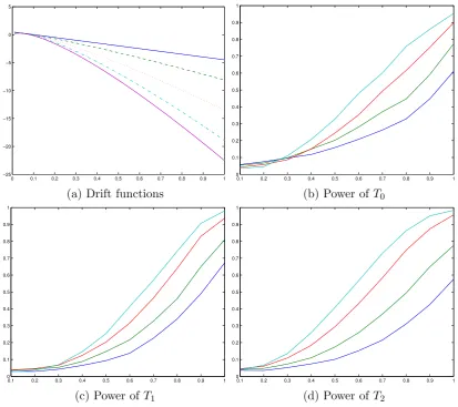
Figure 1 shows the differences of the drift functions between the null model and the
alternative models. It also gives the 5% level power functions of the three tests at the 4
different sample sizes. All the three tests show increasing power as the sample size grows
large, confirming the consistency result of the tests. The performance of the three tests
seems to be similar for this type of deviations in the drift function.
6.2.2 Misspecification in the diffusion function
Here we consider the misspecification in the diffusion function of the volatility process.
The null model is still the Heston model (7). In the alternative model, the drift function
remains the same, but the diffusion function corresponds to a GARCH diffusion process.
dσt2 =α(β−σt2)dt+{(1−τ)γpσ2
t +τ ρ(σ
2
0 0.1 0.2 0.3 0.4 0.5 0.6 0.7 0.8 0.9 1 −25
−20 −15 −10 −5 0 5
(a) Drift functions
0.1 0.2 0.3 0.4 0.5 0.6 0.7 0.8 0.9 1 0
0.1 0.2 0.3 0.4 0.5 0.6 0.7 0.8 0.9 1
(b) Power of T0
0.1 0.2 0.3 0.4 0.5 0.6 0.7 0.8 0.9 1 0
0.1 0.2 0.3 0.4 0.5 0.6 0.7 0.8 0.9 1
(c) Power ofT1
0.1 0.2 0.3 0.4 0.5 0.6 0.7 0.8 0.9 1 0
0.1 0.2 0.3 0.4 0.5 0.6 0.7 0.8 0.9 1
[image:17.595.90.504.71.438.2](d) Power of T2
Figure 1: Power under misspecification of the drift function. (a): drift function with
τ = 0 (solid), τ = 0.2 (dashed), τ = 0.5 (dotted), τ = 0.8 (dash-dotted), τ = 1 (purple solid). (b), (c), (d): n = 500 (blue),n= 1000 (green), n = 2000 (red),n = 3000 (cyan).
for τ = 0,0.1, . . . ,1, where ρ(σ2t) = cσt2 with c = 5. When τ = 1, the alternative model is a GARCH diffusion process.
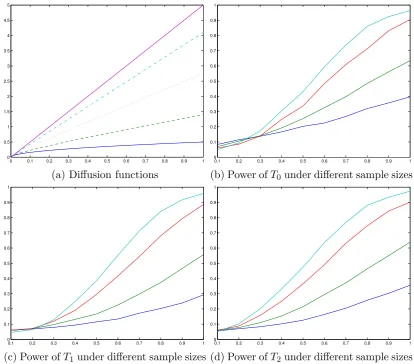
Figure 2 shows the differences of the diffusion functions between the null model and the alternative models. It also gives the 5% level power functions of the three tests at
the 4 different sample sizes. Again all the three tests show increasing power (to 1) as the
sample size grows large. The power of T0 seems to be slightly better than T2 when the
deviation is small, while when the deviation is large, the power seems to be similar.
6.2.3 Jumps in the volatility process
We now consider the power of the three tests against a sequence of models where the volatility process contains jumps
dσ2t =α(β−σt2−)dt+γ
q
σ2
t−dWt+ξ
v
0 0.1 0.2 0.3 0.4 0.5 0.6 0.7 0.8 0.9 1 0
0.5 1 1.5 2 2.5 3 3.5 4 4.5 5
(a) Diffusion functions
0.1 0.2 0.3 0.4 0.5 0.6 0.7 0.8 0.9 1 0
0.1 0.2 0.3 0.4 0.5 0.6 0.7 0.8 0.9 1
(b) Power ofT0 under different sample sizes
0.1 0.2 0.3 0.4 0.5 0.6 0.7 0.8 0.9 1 0
0.1 0.2 0.3 0.4 0.5 0.6 0.7 0.8 0.9 1
(c) Power ofT1under different sample sizes
0.1 0.2 0.3 0.4 0.5 0.6 0.7 0.8 0.9 1 0
0.1 0.2 0.3 0.4 0.5 0.6 0.7 0.8 0.9 1
[image:18.595.89.504.71.435.2](d) Power ofT2 under different sample sizes
Figure 2: Power under misspecification of the diffusion function. (a): drift function with
τ = 0 (solid), τ = 0.2 (dashed), τ = 0.5 (dotted), τ = 0.8 (dash-dotted), τ = 1 (purple solid). (b), (c), (d): n = 500 (blue),n= 1000 (green), n = 2000 (red),n = 3000 (cyan).
where σ2
t− := lims↑tσ
2
s,Ntv is a Poisson process with intensityλv, ξv is the jump size
fol-lowing an exponential distribution, independent of (Wt) and (Bt). We use the Compound
Poisson type, large and infrequent, jump specification for the volatility jumps, which is
a stylized fact observed for daily level equity or equity index data. We consider 5 jump
intensities: 0.5, 1, 1.5, 2, 2.5 and 3. These numbers can be understood as the average
number of jumps in a year. The jump intensity values are based on the estimation result
in Eraker et al. (2003) for the S&P 500 data, where the estimated jump intensity is 1.5 jump per year with a standard deviation of 0.5 jump per year. The jump size ξy is
ex-ponentially distributed with mean 0.2, corresponding to a 20% average sized jump. The
jump size distribution and parameter are also chosen based on the model and estimation
results in Eraker et al. (2003). Figure 3 gives the power functions of the three tests under
different sample sizes. We observe again the consistency of the three tests for this type of
process increases, the tests are more powerful in detecting the deviations. The relative
performance of the three tests seems to be similar to this type of deviations.
0.5 1 1.5 2 2.5 3
0.1 0.2 0.3 0.4 0.5 0.6 0.7 0.8 0.9 1
(a) Power of T0
0.5 1 1.5 2 2.5 3
0.1 0.2 0.3 0.4 0.5 0.6 0.7 0.8 0.9 1
(b) Power of T1
0.5 1 1.5 2 2.5 3
0.1 0.2 0.3 0.4 0.5 0.6 0.7 0.8 0.9 1
[image:19.595.89.504.119.482.2](c) Power ofT2
Figure 3: Power under different volatility jump intensities. (a), (b), (c): n= 500 (blue),
n= 1000 (green), n = 2000 (red),n = 3000 (cyan).
6.2.4 Jumps in the price process
We now consider the power of the three tests when the alternative model have jumps in
the price process.7 To be specific, we consider a sequence of alternative models having a
Poisson-type jump in the price process with jump sizeξty following a normal distribution, while the volatility model is correctly specified:
dYt=σtdBt+ξydNty,
dσt2 = 5(0.1−σ2t)dt+ 0.75pσ2
tdWt,
(11)
whereNty is a Poisson process with jump intensityλy,ξy follows i.i.d. normal distribution
with mean µy and standard deviation σy. We set ρ = −0.4, µy = −0.1 (an average
price jump is -10% on an annual basis) and σy = 0.1. The price jump size distribution
and its parameters are based on the specification used in Eraker et al. (2003) and the
estimation results therein. A negativeµy is in line with empirical observation as most of
the price jumps are downwards. The sequence of models we consider have different jump
intensities: λy = 5,10,15,20,25,30. Figure 4 gives the power functions of the three tests under different sample sizes. We observe again the monotonic increase in power of the
three tests for this type of deviations to the null hypothesis. Again as the jump intensity
of the price process increases, the deviations are easier to identify. The distribution function based test seems more powerful than the density function based test for this
type of deviations.
By comparing the power results for price jump deviations and the volatility jump
deviations in Section 6.2.3, we have also found some interesting results on how the return
distribution is affected differently by these two types of jumps. In Section 6.2.3 we have
seen that the power of the three tests are close to 1 when the volatility jump intensity is
close to 3 (on average 3 jumps a year); while in this section, the power of all the tests
get close to 1 when the jump intensity is close to 30 (on average 30 jumps a year). This
clearly means that the return distribution based tests are more sensitive to volatility jumps, hinting that jumps in volatility have a large effect on the return distribution.
Considering the modelling implication of the two types of jumps we find that the
obtained results are reasonable: volatility jumps, even if they only happen a few times
a year, will bring persistent change to the volatility process as it needs to revert to its
long-run mean for an extended period of time, which will cause substantial distortion
to the return distribution. While price jumps, if they only happen a few times a year,
even when the jump size is large, only add a couple of “outliers” to the tail of the return
distribution and will not have a big influence on the shape of the return distribution. Only
when the jump intensity is high enough (30 here), the tail part will receive enough mass and the change in the return distribution will become obvious. The testing results echo
the comments made in Eraker et al. (2003) that “the volatility jumps bring persistent
change to the returns and price jumps bring transient changes...”, but they also provide
a concrete and transparent illustration of the difference.
6.3
Power performance of the tests in a more general model
Section 5 has discussed that the tests developed in this paper can be used to test more
general models. To study the robustness of the power performance of the three tests in
5 10 15 20 25 0
0.1 0.2 0.3 0.4 0.5 0.6 0.7 0.8 0.9 1
(a) Power of T0
5 10 15 20 25
0 0.1 0.2 0.3 0.4 0.5 0.6 0.7 0.8 0.9 1
(b) Power of T1
5 10 15 20 25
0 0.1 0.2 0.3 0.4 0.5 0.6 0.7 0.8 0.9 1
[image:21.595.89.504.70.434.2](c) Power ofT2
Figure 4: Power under different price jump intensities. (a), (b), (c): n = 500 (blue),
n= 1000 (green), n = 2000 (red),n = 3000 (cyan).
subsection in a model with leverage effect.
To be specific, in the null model (1) the Brownian motions {Wt}t≥0 and {Bt}t≥0 now
correlated with a coefficient ρ=−0.4. We consider the same 4 types of deviations as in (8), (9), (10) and (11) in Section 6.2, the corresponding power plots are given in Figure
1-4 of the online appendix to this paper to save space. The simulation results show that,
7
Empirical applications
7.1
Apple stock, 2000–2014
In this section, we apply our tests to a daily Apple stock price dataset, with the purpose of
illustrating the use of the tests proposed in this paper. The dataset contains the adjusted
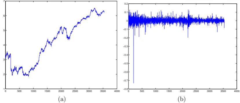
closing prices from January 3rd, 2000 to February 3rd, 2014, making 3543 observations
in total. Figure 5 gives the plot of the log-price levels and log-returns.
0 500 1000 1500 2000 2500 3000 3500 4000 1
2 3 4 5 6 7
(a)
0 500 1000 1500 2000 2500 3000 3500 4000 −0.8
−0.7 −0.6 −0.5 −0.4 −0.3 −0.2 −0.1 0 0.1 0.2
(b)
Figure 5: (a): Log prices of Apple stock, 2000–2014. (b): Log returns of Apple stock, 2000–2014.
The Heston model (7) is fitted to the data, using the GMM approach of Meddahi
(2002). The estimated parameters are ˆα = 17.5119, ˆβ = 0.1793, ˆγ = 2.4715. We then
apply the nonparametric specification tests proposed in this paper to study the validity of
the Heston model. We still use the cross-validation method to determine the bandwidth
and use the Gaussian kernel. Based on 1000 bootstrap samples, the estimatedp-values for
T0,T1 andT2 are 0.009, 0.014 and 0.000 respectively. Thep-values of all the tests provide
strong evidence of rejection of the Heston model. The p-value of the distribution-based
test is smaller than the p-values of the other two tests.
Although it is well-known that the Heston model is misspecified for many return series,
the results of this empirical application provides evidence that the model misspecification
(partly) comes from the misspecification in the marginal distribution of the model. We
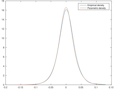
also give a plot of the nonparametrically estimated density of Apple returns and the
cor-responding model implied density in Figure 6. Although the parametric density provides
a reasonable fit to the empirical density, our tests results show that the discrepancy is large enough to reject the model. Also, the parametric density seems to exhibit a slight
[image:22.595.87.502.216.394.2]p-value for the distribution function based test and the known results in nonparametric
tests that the distribution function based tests are in general more sensitive to global
shifts of the whole distribution. The location shift could be caused by a combination
of price jumps and leverage effects, although the skewness and excess kurtosis in the
empirical density (relative to the parametric density) are not very large.
-0.2 -0.15 -0.1 -0.05 0 0.05 0.1 0.15
0 2 4 6 8 10 12 14 16 18
[image:23.595.113.481.174.461.2]Empirical density Parametric density
Figure 6: Nonparametric and parametric density estimates of Apple returns.
7.2
Eraker et al. (2003)’s models of S&P 500 returns
The Heston model is popular in empirical finance and has been used widely in option
pricing. However, the statistical fit of the Heston model has long been questioned; one
reason is that it has limited capacity in modelling the large movements in empirical
returns. Towards a more realistic model for the stock price, Bakshi et al. (1997), Bates
(2000), Andersen et al. (2002) and Pan (2002), among others, have included jump terms in the price process. The empirical results in Bakshi et al. (1997) and Bates (2000) have
also pointed to the possible existence of jump terms in the volatility process. Eraker et al.
(2003) have advanced the empirical literature of stochastic volatility in this direction by
considering stochastic volatility models with jumps in both the price process and the
volatility process. They estimate the model with a likelihood based method implemented
of volatility jumps. To be specific, Eraker et al. (2003) have fitted 20 years of S&P
500 equity index data to four models, namely a stochastic volatility model (SV), which
is essentially the Heston model; a stochastic volatility model with price jumps (SVJ);
a stochastic volatility model with correlated price and volatility jumps (SVCJ); and a
stochastic volatility model with independent price and volatility jumps (SVIJ). Eraker
et al. (2003) have found that the models with jumps in price and volatility (both the
SVIJ and the SVCJ model) have the best fit.
Although Eraker et al. (2003) have used several diagnostics to test the validity of their
models, none of these has considered the validity of the model implied return distribution.
Treating the estimated models as specific models, we apply our tests to study the validity of the model implied return distributions using the methodology discussed in Section 5.
Since the SVIJ model and the SVCJ model exhibit very similar properties in all the
diagnostics in Eraker et al. (2003), with the SVIJ model performing slightly better, we
thus only study the SVIJ model, together with the SV model and the SVJ model. We
acquire the same S&P 500 index data from January 2, 1980 to December 31, 1999, and
test the estimated model with these data.
Since our tests are based on the density function and the distribution function of the
return data, we first give a plot of the empirical density function estimated and all the
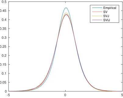
model implied return densities in Figure 7. The empirical density is estimated using a kernel density estimator with the bandwidth selected by the cross-validation method. It
is seen that there are some discrepancies between the empirical density and the model
implied densities, especially at the left tail and around the peak. The SV model implies a
return density with a lower peak than the empirical density, its distance to the empirical
density is also the largest in the left tail. The SVJ model improves upon the SV model
both in the peak of the density and in the left tail. One surprising observation is that the
SVIJ model does not seem to improve the distributional fit of the returns upon the SVJ
model: the peak of the SVIJ model implied density is even slightly further away from
the empirical density than the SV model, but the SVIJ model does seem to improve the fit of the left tail over the SV model, and has a left tail indistinguishable from the SVJ
model. Visual inspection suggests that the SVJ model probably provides the best fit to
the empirical density. We next apply the statistical tests developed in this paper to see
if this is indeed the case.
We apply the three tests to the three estimated models and calculate thep-values of the
tests based on the parametric bootstrap method. Cross-validation is used to determine
the bandwidth and 1000 parametric bootstrap replications are used. Thep-values for the
three tests for the SV model, the SVJ model and the SVIJ model are given in Table 2.
-5 0 5 0
0.05 0.1 0.15 0.2 0.25 0.3 0.35 0.4 0.45 0.5
[image:25.595.96.500.72.395.2]Empirical SV SVJ SVIJ
Figure 7: Empirical density of S&P 500 daily returns and model implied return densities.
T0 T1 T2
SV 0.029 0.033 0.017
SVJ 0.189 0.194 0.129
SVIJ 0.039 0.040 0.022
Table 2: p-values of all the tests for the models in Eraker et al. (2003).
densities. The SV model implied density is too far from the empirical density, thus is
rejected significantly at the 5% level. The SVJ model improves over the SV model, and
we don’t find enough statistical evidence to reject the density implied by it, even using
a 10% significance level. Our tests confirm that the SVIJ model implied return density
is worse than that implied by the SVJ model, it is not favoured by all three tests and is
rejected significantly at the 5% level.
With these test results, we find some new evidence on the statistical fit of the
mod-els considered in Eraker et al. (2003). As discussed in Eraker et al. (2003), page 1274,
“models with only jumps in returns and diffusive stochastic volatility can generate
real-istic patterns of both unconditional and conditional nonnormalities ...”. Our test results
distribution. They also write, “... but they (return jumps) have difficulty capturing the
dynamics of the conditional volatility of returns,” for which jumps in the volatility would
probably be needed. Here, Eraker et al. (2003) have discussed the potential improvement
offered by the SVIJ model. From our evidence, however, we remark that even if the SVIJ
model could potentially improve the fit of the conditional return distribution (dynamics
of conditional volatility), this improvement does not come without any costs: introducing
the volatility jump factor leads to a worse fit of the unconditional distribution relative to
the SVJ model.
8
Conclusion and extensions
We propose three tests for stochastic volatility model specification by comparing the
parametrically and nonparametrically estimated stationary marginal density functions
and distribution functions of the observed returns. The consistency of the three tests are
derived and we have studied their finite sample power property under various alternative
models. In empirical applications, our tests provide some new insights in the model
misspecification issue of some popular stochastic volatility models.
To consider extensions, our approach can be adapted to discrete-time stochastic volatility models easily, as long as the volatility process is stationary and β-mixing as
assumed in this paper. One can then compare the estimated density functions and
distri-bution functions as discussed for continuous-time models analogously. Another possible
extension to consider is to formulate the test statistics based on the conditional
distribu-tion of returns: as discussed in the introductory secdistribu-tion, the stadistribu-tionary marginal return
distribution does not contain information on the dynamics in the data. To exploit the
dependence structure in the model, we could extend our approach to the one-step
con-ditional distribution function and density function of Xi|Xi−1, i = 2, . . . , n, to formulate
Appendix A: Basic setup and probabilistic properties
(N1) (kernel function) The kernel function K is a bounded, symmetric, nonnegative
function on R, satisfying
Z ∞
−∞
K(x)dx= 1,
Z ∞
−∞
xK(x)dx= 0,
Z ∞
−∞
x2K(x)dx= 2k <∞,
where k >0 is a constant, and
Z ∞
−∞
K2(x)dx <∞.
(N2) (density function)q(x) and its second order derivative are bounded and uniformly
continuous on R.
The above assumptions on the kernel function, and the smoothness assumption on the
density function are not the weakest possible. However, Assumptions (N1) and (N2) are
sufficient for the present purpose and simplify the argument in the proof.
(N3) For the process (Xi)ni=1, all two dimensional joint densities of (X1, . . . , Xn) exist, are
bounded and Lipschitz continuous. This implies that the corresponding distribution functions satisfy the same conditions.
(N4) As n → ∞,hn →0 and nhn → ∞.
These set of conditions will be used to derive the asymptotic properties of the test
statis-tics, but together with the mixing conditions we assume throughout, they are also
suffi-cient to make ˆq(x) a (pointwise) consistent estimator ofq(x) for all x∈R.
The tests developed in this paper require the observed return sequence to be
station-ary, ergodic andβ-mixing with exponentially decaying coefficients. In the nonparametric
model, it is sufficient to assume the observed return sequence (Xi)ni=1 to satisfy the above
conditions directly. However, in the parametric model, it is non-trivial to check that
these conditions are satisfied for particular choices of the functions b(x;θ) and a(x;θ). In
the parametric stochastic volatility model (1), we first assume
(SV0) (B, W) is a standard Brownian motion in R2, defined on the probability space
(Ω,F,P), and σ2
0 is random variable defined on the same probability space,
inde-pendent of (B, W).
(SV1) For all θ ∈ Θ, the function b(x) = b(x;θ) is continuous on (0,+∞), and the function a(x) =a(x;θ) is continuously differentiable on (0,+∞), such that
∃K >0, ∀x >0, b2(x) +a2(x)≤K(1 +x2),
and
∀x >0, a(x;θ)>0.
This assumption ensures the existence and uniqueness of an almost surely positive strong
solution to the stochastic differential equation (1) generating the volatility process.
Define, for v0 >0, thescale measure
s(x;θ) = exp
−2
Z x
v0
b(v;θ)
a2(v;θ)dv
,
and thespeed measure
m(x;θ) = 1
a2(x;θ)s(x;θ).
Then the assumption
(SV2)
Z ·
0
s(x;θ)dx=∞,
Z ∞
·
s(x;θ)dx=∞,
Z ∞
0
m(x;θ)dx=M < ∞,
where the · in the integral means an arbitrary point in the domain of s(x;θ), ensures a unique and positive recurrent solution on (0,∞), see Genon-Catalot et al. (1998).
The last condition in (SV2) guarantees the existence of a stationary distribution (for
the volatility process), with density defined as
π(x;θ) = m(x;θ)
M I(x >0).
If the process is initiated from this stationary distribution, i.e., under assumption
(SV3) The initial random variable σ02 has density π(x;θ),
the solution is strictly stationary and ergodic.
Now we give sufficient conditions to ensure that the volatility process is β-mixing
with exponentially decaying coefficients. From Theorem 3.6 of Chen et al. (2010), a
sufficient condition (together with (SV1) and (SV2)) for exponential decay of theβ-mixing
coefficients is that the process is ρ-mixing, so in the following we give the conditions for
the process to beρ-mixing. Also, we note the result that if a diffusion process isρ-mixing,
Genon-Catalot, Jeantheau, and Laredo (2000), Proposition 2.5). Furthermore, β-mixing
andρ-mixing with exponential decay are almost equivalent concepts for scalar diffusions,
as discussed in Chen et al. (2010).
(SV4)
lim
x↓0 a(x;θ)m(x;θ) = 0, xlim↑∞a(x;θ)m(x;θ) = 0.
(SV5) Let
γ(x;θ) =a0(x;θ)−2b(x;θ)
a(x;θ);
the limits of 1/γ(x;θ), as x↓0 and as x↑ ∞, exist.
Appendix B: Lemmas and proofs
The conditions in Appendix A ensure strict stationarity, ergodicity and β-mixing of the
volatility process. Notice that the return sequence (Xi)ni=1 is a sequence of stochastic
integrals of the volatility process with respect to an independent Brownian motionB over
small fixed intervals. By the following lemma from Zu (2015), the return series inherit
the stationarity, ergodicity and the β-mixing properties from the volatility process.
Lemma 1 In the model (1), if the volatility process (σ2
t)t≥0 is stationary, ergodic and β-mixing with a certain decay rate, then the normalized return sequence (Xi)ni=1 is also stationary, ergodic and β-mixing, with a mixing decay rate at least as fast as that of
(σ2t)t≥0.
In all the proofs in this appendix, we take the above mentioned probabilistic properties for the return series as given to avoid repetition. When we use an integral without the
range of integration, the integration is over the full real axisR.
Proof (of Theorem 1) We first derive the asymptotic distribution of T0. Notice that
T0
= nh1/2
Z
(ˆq(x)−Kh ∗q(x; ˆθn))2dx
= nh1/2
Z
(ˆq(x)−Kh ∗q(x))2dx+nh1/2
Z
(Kh∗q(x)−Kh∗q(x; ˆθn))2dx
+nh1/2
Z
(ˆq(x)−Kh∗q(x))(Kh∗q(x)−Kh∗q(x; ˆθn))dx.
Define
T00 =nh1/2
Z
It will be shown later that T00 = Op(1); the second term nh1/2
R
(Kh ∗ q(x) − Kh ∗
q(x; ˆθn))2dx =Op(h1/2) because ˆθn is a
√
n-consistent estimator of θ0 and by the square
integrable assumption on the Lipschitz constant L(x) as in Assumption (P1a), so this
term is dominated byT00; the crossproduct term is clearly dominated byT00 by the
Cauchy-Schwarz inequality. Thus we have that
T0 =T00(1 +op(1)),
and we derive the asymptotic distribution of T00 in the following.
First notice Z 1 n n X i=1
(Kh(x−Xi)−Kh∗q(x))
!2 dx = 1 n2 n X i=1 Z
(Kh(x−Xi)−Kh∗q(x))2dx
+ 2
n2
X
i<j
Z
(Kh(x−Xi)−Kh ∗q(x))(Kh(x−Xj)−Kh∗q(x))dx
:= 1
n2
n
X
i=1
ϕn(Xi, Xi) +
2
n2
X
i<j
ϕn(Xi, Xj),
where
ϕn(u, v) :=
Z
(Kh(x−u)−Kh∗q(x))(Kh(x−v)−Kh ∗q(x))dx.
Next, we show that
1. The sum of the diagonal terms
1
n2
n
X
i=1
ϕn(Xi, Xi) p
−
→(nh)−1
Z
K2(u)du.
2. The sum of the off-diagonal terms
nh1/2 2 n2
X
i<j
ϕn(Xi, Xj)
!
d
− →N
0,2
Z
q02(u)du
Z
(K(2)(u))2du
.
3. Then we show that
T00 −→d N
0,2
Z
q02(u)du
Z
(K(2)(u))2du
,
Step 1 We first compute the order of the mean, E 1 n2 n X i=1
ϕn(Xi, Xi)
!
= 1
nEϕn(X1, X1)
= 1
n
Z Z
(Kh(x−X1)−Kh∗q(x))2dxq(X1)dX1
= 1
nh2
Z Z
K
x−X1 h
2
q(X1)dxdX1(1 +o(1))
= 1
nh
Z Z
(K(u))2q(X1)dudX1(1 +o(1))
= (nh)−1
Z
K2(u)du(1 +o(1)). (12)
Then we compute the order of the variance
Var 1
n2
n
X
i=1
ϕn(Xi, Xi)
!
6 E 1
n2
n
X
i=1
ϕn(Xi, Xi)
!2
= 1
n3Eϕ 2
n(X1, X1) +
2
n4
X
i<j
Eϕn(Xi, Xi)ϕn(Xj, Xj). (13)
We look at the two terms separately. For the first term
Eϕ2n(X1, X1)
=
Z Z
Kh2(x−X1)dx
2
q(X1)dX1(1 +o(1))
= 1
h4
Z Z
K2
x−X1 h
dx
2
q(X1)dX1(1 +o(1))
= 1
h2
Z Z
K2(u)du
2
q(X1)dX1(1 +o(1))
For the second term,
Eϕn(Xi, Xi)ϕn(Xj, Xj)
=
Z Z Z
Kh2(x−Xi)dx
Z
Kh2(x−Xj)dxq(Xi, Xj)dXidXj(1 +o(1))
= 1
h2
Z Z Z
K2(u)du
2
q(Xi, Xj)dXidXj(1 +o(1))
= O 1 h2 . (15)
Use the result in (14) and (15) in (13), we get
Var 1
n2
n
X
i=1
ϕn(Xi, Xi)
!
6 1
n3O
1
h2
+ 2
n4n 2O 1 h2 = O 1
n2h2
. (16)
Use the results in (12) and (16) and apply Markov’s inequality we have
P 1 n2 n X i=1
ϕn(Xi, Xi)−(nh)−1
Z
K2(u)du
> ε ! 6 E n12
Pn
i=1ϕn(Xi, Xi)−(nh) −1R
K2(u)du 2 ε2 = O 1
n2h2
=o(1),
because nh→ ∞. Thus we have proved that
1
n2
n
X
i=1
ϕn(Xi, Xi)−(nh)−1
Z
K2(u)du = op(1).
Step 2 Now we use Theorem A, Appendix 1 in Hjellvik, Yao, and Tjøstheim (1998) to
show
nh1/2 2 n2
X
i<j
ϕn(Xi, Xj)
!
d
− →N
0,2
Z
q02(u)du
Z
(K(2)(u))2du
.
Notice that ϕn(x, y) is a degenerate symmetric kernel, and the mixing condition is
satis-fied.
the same distribution asXi. First we compute
Eϕ2n( ˜Xi,X˜j)
=
Z Z Z
Kh(x−Xi)Kh(x−Xj)dx
2
q(Xi)q(Xj)dXidXj(1 +o(1))
= 1
h2
Z Z Z
K(u)K
u+Xi−Xj
h
dx
2
q(Xi)q(Xj)dXidXj(1 +o(1))
= 1
h2
Z Z
K(2)
Xi−Xj
h
2
q(Xi)q(Xj)dXidXj(1 +o(1))
= 1
h
Z Z
(K(2)(u))2q(Xj+uh)q(Xj)dudXj(1 +o(1))
= 1
h
Z
(K(2)(u))2du
Z
q2(x)dx(1 +o(1)).
then the asymptotic variance is
σn2 = n
2
2 Eϕ
2
n( ˜Xi,X˜j) =
n2
2h
Z
(K(2)(u))2du
Z
q2(x)dx(1 +o(1)). (17)
Then we check the conditions related to the 6 quantities Mni, i= 1, . . . ,6, as defined
in Theorem A, Appendix 1 in Hjellvik, Yao, and Tjøstheim (1998). ForMn1, notice that
for 1> δ >0,
E|ϕn(X1, Xj)ϕn(Xi, Xj)|1+δ
=
Z Z Z
Z
Kh(x−X1)Kh(x−Xj)dx
Z
Kh(x−Xi)Kh(x−Xj)dx
1+δ
q(X1, Xi, Xj)dX1dXidXj(1 +o(1))
=
Z Z Z
1 h4 Z K
x−X1 h
K
x−Xj
h dx Z K
x−Xi
h
K
x−Xj
h dx 1+δ
q(X1, Xi, Xj)dX1dXidXj(1 +o(1))
=
Z Z Z
1
h2K (2)
X1−Xj
h
K(2)
Xi−Xi
h 1+δ
q(X1, Xi, Xj)dX1dXidXj(1 +o(1))
= h2
Z Z Z
1
h2K
(2)(u)K(2)(v)
1+δ
q(Xj +uh, Xj+vh, Xj)dudvdXj(1 +o(1))
= 1
h2δ
Z
|K(2)(u)|1+δdu
2Z
q(Xj +uh, Xj+vh, Xj)dXj(1 +o(1))
= O
1
h2δ
.
have
n2M
1 1+δ
n1 /σ 2
n=O
h h2δ/(1+δ)
=Oh11+−δδ
=o(1).
Similarly, we can show that
E|ϕn(X1, Xj)ϕn(Xi, Xj)|2(1+δ) = O
h2 h4(1+δ)
=O
1
h4δ+2
,
E|ϕn(X1, Xj)ϕn(Xi, Xj)|2 = O
1
h2
,
E|ϕn(X1, Xi)ϕn(Xj, Yk)|2(1+δ) = O
1
h4δ+2
,
which further imply that
n32M 1 2(1+δ)
n2 /σ 2
n =O
1
n1/2hδ/(1+δ)
=o(1),
n32M 1 2
n3/σ 2
n=O
1
n1/2
=o(1).
n32M 1 2(1+δ)
n4 /σ 2
n =O
1
n1/2hδ/(1+δ)
=o(1),