Uncertain information combination for decision making in smart grid BDI agent systems

1

Uncertain Information Combination for Decision Making in Smart Grid

BDI Agent Systems

Sarah Calderwood, Kevin McAreavey, Weiru Liu, Jun Hong

School of Electronics, Electrical Engineering and Computer Science,

Queen’s University Belfast, United Kingdom

{scalderwood02, kevin.mcareavey, w.liu, j.hong} @ qub.ac.uk

Abstract

In a smart grid SCADA (supervisory control and data acquisition) system, sensor information (e.g. temperature, voltage, frequency, etc.) from heterogeneous sources can be used to reason about the true system state (e.g. faults, attacks, etc.). Before this is possible, it is necessary to combine information in a consistent way. However, information may be uncertain or incomplete while the sensors may be unreliable or conflicting. To address these issues, we apply Dempster-Shafer (DS) theory to model the information from each source as a mass function. Each mass function is then discounted to reflect the reliability of the source. Finally, relevant mass functions (after evidence propagation) are combined using a context-dependent combination rule to produce a single combined mass function used for reasoning. We model a smart grid SCADA system in the belief-desire-intention (BDI) multi-agent framework to demonstrate how our approach can be used to handle the combined uncertain sensor information. In particular, the combined mass function is transformed into a probability distribution for decision-making. Based on this result, the agent can determine which state is most plausible and insert a corresponding AgentSpeak belief atom into its belief base. These beliefs about the environment affect the selection of predefined plans, which in turn determine how the agent will behave. We also identify conditions when a combination should occur to ensure the reactiveness of the agent.

Keywords-Dempster-Shafer theory; information fusion, context-dependent combination; BDI; AgentSpeak; uncertain beliefs.

1. Introduction

Supervisory control and data acquisition (SCADA) systems [1] are deployed in a variety of environments including power [2] and water treatment [3]. Such systems monitor and control machinery and devices through gathering and analysing real time sensor information. In a power setting, sensors independently gather information about the environment such as temperature, voltage,

frequency, wind speed/direction, etc. to help pinpoint faults, perform network modelling, simulate power operation and preempt outages. Complex SCADA systems can be modelled using the Belief-Desire-Intention (BDI) multi-agent framework [8] for programming intelligent agents. Each agent in the BDI framework is modelled by its (B)eliefs (its current belief state), (D)esires (what it wants to achieve) and (I)ntentions (desires it has chosen to act upon). However, BDI implementations cannot deal with information which is uncertain or incomplete (e.g. due to noisy measurements) while the sensor themselves may be unreliable or conflicting (e.g. due to malfunctions). As such, it is important to accurately model and combine this information to ensure higher-level decision making in an uncertain dynamic environment.

2

The remainder of our work is organized as follows. In Section 2, we introduce the preliminaries on DS theory and AgentSpeak. In Section 3, we provide a smart grid scenario and discuss how uncertain information can be modelled. In Section 4, we provide an outline of a context-dependent combination rule and in Section 5 we discuss how to handle uncertain beliefs in AgentSpeak. Section 6 provides details of our implementation in AgentSpeak. In Section 7, we discuss related work. Finally, in Section 8 we draw our conclusions.

2. Preliminaries

In this section, we begin by introducing the preliminaries on Dempster-Shafter theory [4] followed by the preliminaries on the AgentSpeak framework [9] for BDI agents.

2.1. Dempster-Shafer theory

Dempster-Shafer (DS) theory is capable of dealing with incomplete and uncertain information. The frame of discernment Ω = {ω1,…,ωn} is defined as a mutually exclusive and exhaustive set of possible hypotheses where one is true at a particular time. A mass function is a mapping m : 2Ω _{→ [0,1]} that satisfies the conditions m(∅) = 0 and ΣA⊆Ω m(A)

= 1. Intuitively, m(A) defines the proportion of evidence that supports A, but none of its strict subsets.

To reflect the reliability of a source we apply a discounting factor α 𝜖 [0,1] using Shafer’s discounting technique [4] for a mass function m over

Ω. A discounted mass function mα _{is defined for each}

A⊆Ω as:

where α = 0 represents a totally reliable source and α = 1 represents a totally unreliable source. Once a mass function has been discounted it can then be treated as fully reliable.

When considering a set of independent and reliable sources, several ways of combining mass functions have been proposed. One of the best known rules to combine mass functions is Dempster’s rule of combination [4], denoted mi ⨁

mj, which is defined as:

with c a normalization constant, given by c = 1/1-K(mi, mj) with K(mi, mj) = ΣB⋂C=∅ mi(B)mj(C). The effect of the normalization constant c, with

K(mi, mj) the degree of conflict between miand mj, is to redistribute the mass value assigned to the empty set. As such, Dempster’s rule is not well suited to combine mass functions with a high degree of conflict. In this paper, we use the K(mi, mj) value as a conflict measure to determine the context for using Dempster’s rule. Dubois and Prade’s

disjunctive consensus rule [7], on the other hand, denoted mi ⨂ mj, is defined as:

Notably, the disjunctive rule omits normalisation and incorporates all conflict. As such, this rule is suitable to combine mass functions with a high degree of conflict.

The ultimate goal of representing and reasoning about uncertain information is to draw conclusions from it. Smet’s pignistic model [11] allows decisions to be made on individual hypotheses. A mass function m on Ω is transformed into a pignistic probability distribution such that:

To ensure compatible sources will return strictly compatible mass functions (i.e. mass functions defined over the same frame), we use evidential mapping [12] on frames Ωe and Ωh where Γ : Ωe x 2Ωh

→ [0,1] is an evidential mapping from Ωe and Ωh that satisfies the conditions ω ϵ Ωe, Γ(ωe, ∅) = 0 and

ΣH⊆Ωh Γ(ωe, H) = 1. Furthermore, if we have frames

Ωe and Ωh, with me a mass function over Ωe and Γ an evidential mapping from Ωe to Ωh, then a mass function mh over Ωh is an evidence propagated mass function from me with respect to Γ and is defined for each H ⊆ Ωh in [12] as:

where:

Γ∗_{(E, H) =}

{

∑ Γ(ωe, H) |E| , ωe∈E

𝑖𝑓 𝐻 ≠ ⋃ HE and ∀ωe∈ E, Γ(ωe, H) > 0,

1 − ∑ Γ∗_{(E, H}′₎

H′_{∈ HE} ,

if H = ⋃ HE and ∃ωe∈ E, Γ(ωe, H) = 0,

1 − ∑ Γ∗_{(E, H}′_{) + ∑} Γ(ωe, H) |E| ωe∈E

H′∈ HE

,

if H = ⋃ HE and ∀ωe∈ E, Γ(ωe, H) > 0, 0, otherwise

such that HE = {H’⊆ Ωh | ωe ∈ E, Γ(ωe, H’) > 0} and ⋃ HE = { ωh ∈ H’ | H’ ∈ HE}.

(mi⊗ mj )(A) = ∑ mi(B)mj(C) B∪C=A

m∝_{(A) = {} (1−∝) ∙ m(A), if A ⊂ Ω,

α + (1 − α) ∙ m(A), if A = Ω

BetPm(ω) = ∑ m(A)_|A|

A⊆ Ω,ωϵA

mh(H) = ∑ me(E)Γ∗(E, H) E⊆ Ωe

(mi⊕ mj)(A)

= { 𝑐 ∑B∩C=Ami(B)mj(C), if A ≠ 0,

3

2.2. AgentSpeak

We use S to denote a finite set of symbols for predicates, actions, and constants, and V to denote a set of variables. Following convention, elements from S and V are written using lowercase letters and uppercase letters, respectively. We use the standard first-order logic definition of a term and t as a compact notation for t1,…,tn. From [9], the syntax of the AgentSpeak language is defined as follows:

Definition 1 If b is a n-ary predicate symbol then

b(t) is a belief atom.

Definition 2 If b(t) and c(s) are belief atoms, then

b(t), ¬b(t) and b(t)∧c(s) are beliefs. If g(t) is a belief atom, then !g(t) and ?g(t) are goals with !g(t)

an achievement goal and ?g(t) a test goal.

Definition 3 If b(t) is a belief atom and !g(t) and ?g(t) are goals, then +b(t), -b(t), +!g(t), -!g(t), +?g(t) and -?g(t) are triggering events where + and

– denote addition and deletion events, respectively.

Definition 4 If a is an action symbol and t are terms, then a(t) is an action.

Definition 5 If e is a triggering event, l1,…,lm are belief literals and h1,…,hn are goals or actions, then e:

l1 ∧…∧ lm ← h1,…,hnis a plan where l1 ∧…∧ lmis the

context and h1,…,hnis the body such that ; denotes sequencing.

An AgentSpeak agent A can now be represented as a tuple (Bb, Pl, E, A, I)1 _{where respectively we can} specify an agent by its belief base (a set of belief atoms), plan library (a set of plans to describe how the agent can react to events based on their current beliefs), event set, action set (the primitive actions to which the agent has access) and intention set.

3. Smart grid Scenario

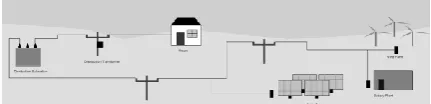
In this section, we introduce a smart grid SCADA system (focusing on solar and wind renewable energy sources) to illustrate our approach. Our scenario consists of six agents: a solar park, a wind farm, a battery storage plant, a distribution substation, a distribution transformer and a house (as shown in Figure 1). The solar park will generate and distribute electric power through high voltage transmission lines to a distribution substation. Here, a transformer will reduce high voltage electric power to low voltage electric power to be distributed across low level distribution lines. A distribution 1 _{For simplicity, we omit three selection functions SE, SO and SI.}

transformer will then convert electric power to lower levels to serve residential loads. However, if a fault or an attack occurs within the solar park or the solar park cannot supply enough electric power to meet demand, electric power will be generated and distributed from a nearby wind farm or provided from a battery storage plant. Each agent also contains a number of sources with various levels of granularity to monitor the overall health of the grid. In the subsection that follows we discuss in further detail the information that may be collected from sources and how it will be modelled.

Figure 1. A smart grid scenario using solar and wind energy sources.

3.1 Modelling uncertain sensor information

In a smart grid SCADA system, sensor information such as temperature, voltage and frequency etc. is obtained from heterogeneous sources to represent the current state of the environment. Notably, given this type of scenario, sensor information will be used to determine if the state of the environment is normal i.e. fully operational or if a fault (with a sensor or component) or security attack is likely to occur. Considering the latter, cyber-attacks can have a negative impact on secure, reliable smart grid SCADA systems, causing blackout and brownouts, issues with instability and unreliability etc. As a result it becomes necessary to identify potential attacks on the system e.g. sensor information may be violated through tampering which leads to disruption in power generation or distribution. As such, we first need to properly model information. For the purpose of illustration, we provide numerical information collected from temperature sensors from the set Ωs = {0,…,40}. In addition, we obtain general estimations from experts such that we have Ωe = {normal, abnormal} to represent normal or abnormal temperature levels. Unfortunately, information from these types of sources may be uncertain due to noisy sensor measurements or experts may not be competent in giving estimations.

4

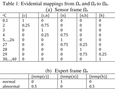
belief base. Table 1 provides the evidential mappings we consider for Ωs and Ωe to Ωh.

Table 1: Evidential mappings from Ωs and Ωe to Ωh.

(a) Sensor frame Ωs

o_{C {c} {c,n} {n} {n,h} {h}}

0,1 2 3 4 5,…,26 27 28 29 30,…,40 1 0.25 0 0 0 0 0 0 0 0 0.75 1 0.25 0 0 0 0 0 0 0 0 0.75 1 0.75 0 0 0 0 0 0 0 0 0.25 1 0.75 0 0 0 0 0 0 0 0 0.25 1

(b) Expert frame Ωe

{temp(c)} {temp(n)} {temp(h)} normal abnormal 0 0.5 1 0 0 0.5

Once information has been obtained it will be modelled as mass functions. Since sources may be unreliable a discounting factor will be applied to derive discounted mass functions that can then be treated as fully reliable.

Example 1. Consider two independent sources S1 and S2 that are located within the solar park and an expert estimation S3. These sources are 85%, 70% and 60% reliable, respectively. Information has been obtained such that S1:[30oC], S2:[26oC, 28oC] and

S3:[normal (70% certain)]. By modelling the (uncertain) information as mass functions we have

m1({30}) = 1, m2({26,…,28}) = 1 and

m3({abnormal}) = 0.7, m3(Ω) = 0.3. By applying the discount factors (i.e. α = 0.15, 0.3 and 0.4

respectively) for S1, S2and S3 we have the following discounted mass functions:

m₁0.15_{({30}) = 0.85, m} 1

0.15_{(Ω) = 0.15,}

m₂0.3_{({26,…,28}) = 0.7, m} 2

0.3_{(Ω) = 0.3,}

m₂₃0.4_{({abnormal}) = 0.42, m} 2 3

0.4_{(Ω) = 0.58.}

We now obtain the following evidence propagated mass functions from the discounted mass functions considering the evidential mappings in Table 1.

Table 2: Evidence propagated mass functions.

m1 m2 m3

m({temp(c)}) m({temp(n),temp(h)}) m({temp(h)}) m(Ω) 0 0 0.85 0.15 0 0.7 0 0.3 0.21 0 0.21 0.58

4. Context-dependent combination

Within the literature we have found existing combination rules are either too restrictive (losing valuable information) or too permissive (resulting in ignorance). To exploit the benefits of different

combination approaches, we use a context-dependent combination rule from [13] to combine a set of mass functions in DS theory. This combination rule determines the context for when we should use Dempster's rule and then resort to Dubois and Prade's rule for a set of relevant mass functions. In particular, we identify a partition of a set of mass functions using a conflict measure in DS theory. This ensures we find subsets with a low degree of conflict. Each element in this partition is called a largely partially maximal consistent subset (LPMCS) and identifies a subset to be combined using Dempster's rule. Once the set of LPMCSes are created and each LPMCS has been combined using Dempster's rule, we then combine the set of highly conflicting LPMCSes using Dubois and Prade's rule. Furthermore, we firstly use heuristics on the quality and similarity of mass functions to ensure LPMCSes are based on high quality information. Specially, we identify the highest quality mass function (using these heuristics) as a reference mass function. Secondly, using the reference mass function we then find the mass function that is closest (i.e. agreement) based on a similarity (distance) measure. Thirdly, the most similar mass function is combined with the reference mass function using Dempster’s rule. Fourthly, the second and third steps are repeated where the combined mass function (the new reference mass function) is combined with its most similar mass function until a threshold level of the conflict measure (i.e. K(mi, mj)

where mi may be m1⨁m2, a reference mass

function and mj is m3, its closest mass function) in DS theory has been exceeded. An LPMCS will therefore contain those mass functions that can be combined before exceeding the threshold.

Example 2. Given the evidence propagated mass functions from Table 2 and a conflict threshold of 0.15, we combine them using the context-dependent combination rule. We obtain the set of LPMCSes {{m1}, {m2, m3}} where m1 ⨂ (m2 ⨁ m3) results in

m({temp(c), temp(h)}) = 0.063, m({temp(n),temp(h)})=0.405, m(Ω) = 0.323, m({temp(h)})=0.209.

5. Handling uncertain beliefs in BDI

5

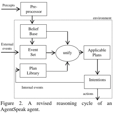
combination that will be added to the agent’s belief base.

Figure 2. A revised reasoning cycle of an AgentSpeak agent.

Classical AgentSpeak is not capable of modelling and reasoning with uncertain information. As such, it becomes necessary to reduce the uncertain information modelled by a mass function to a classical belief atom which can be modelled in the agent’s belief base.

After executing our context-dependent combination rule to obtain a combined mass function and then transforming it into a pignistic probability distribution, the sensor preprocessor of an agent can determine which state is the most plausible by checking if a state exceeds a specified pignistic probability threshold.

Example 3. Assume a pignistic probability threshold of 0.5. After applying pignistic transformation to the result in Example 2, we obtain the following: P(temp(n))=0.31, P(temp(c))=0.139, P(temp(h))=0.551. The solar park agent believes it is more plausible that the temperature is classified as hot than cold or normal

as P(temp(h)) > 0.5. This means the AgentSpeak agent’s belief base is revised with this new belief atom (i.e. temp(h)) and an applicable plan will be selected for this state.

To minimize the computational cost associated with combination we have a condition where the combination rule will only be applied when information obtained from any source has changed significantly (using a distance measure) from a previous reading. However, if no change occurs we also find it necessary to combine and revise information after some specified interval of time.

6. Implementation

In this section we focus specifically on the solar park agent to illustrate how the result of the context-dependent combination rule from Section 4 will aid

plan selection. We use Jason [10], an open-source implementation of the AgentSpeak interpreter to implement the scenario as it implements AgentSpeak’s operational semantics and provides a suitable platform for the development of multi-agent systems.

Example 4. Consider a solar park agent A within the smart grid. Assume the solar park contains four solar panels and a single combiner and inverter. Four solar panels will capture the sun’s energy using photovoltaic cells. The stronger the sunlight the more electric power is produced. The direct current travels along wires connecting the solar panels. The current from all panels is collected via a combiner box. An inverter will convert the direct current power of the four solar panels to alternating current to run the AC loads at household levels. Various sensors are distributed within the solar park to record temperature (e.g. ambient, internal combiner, solar panel temperature), frequency, current, and voltage for monitoring and decision-making purposes.

Each agent’s belief base contains dynamic information such as the result of the combination rule and static information such as that agent’s location. The solar park agent’s belief base may contain the following belief atoms:

(i) temp(n): the temperature is normal (as a result of combining relevant mass functions from temperature sensors);

(ii) freq(n): the frequency is normal (as a result of combining relevant mass functions from frequency sensors);

(iii)solar_park_loc(A,500): agent A’s own location within the smart grid

The solar park agent can perform the following primitive actions:

(i) supply_power: the power is being supplied to the smart grid;

(ii) convert_power: the power is converted from direct DC to AC by the inverter. Each agent has their own individual goals that they strive to achieve individually depending on their state as well as an overall system goal. In the solar park setting, the goal of this agent is to achieve a safe and efficient supply of electrical power to meet consumer demand. The solar park agent also requires communication with other agents to ensure they fulfil their overall goal. This might involve sub-goals such as running the combiner to distribute power when we obtain a normal temperature reading or stopping a combiner and generating an alert when the temperature is classified as e.g. cold or hot. The following AgentSpeak plans are a selection from the solar park agents plan library:

P1: +!prepare_to_start_solar_park_ : true ← calibrate_inverter; calibrate_combiner; !start_solar_park.

environment Percepts

External events

Pre-processor

Belief Base

Event Set

Applicable Plans

Plan Library

Intentions

Internal events

6

P2: +!start_solar_park : not supplying_smart_grid & calibrated_combiner & calibrated_inverter ← !run_combiner; !run_solar_panel_1; !run_solar_panel_2, !run_solar_panel_3; !run_solar_panel_4.

P3: +!run_solar_panel_1 : temp(n) ← collect_protons; !run_combiner; …

P4: +temp(h) : true ← !generate_alert; !stop_combiner; !stop_inverter; !run_windfarm;…

The initial goal of the solar park agent is !prepare_to_start_solar_park. As such, the context within plan P1 is believed to be true and the agent takes the primitive actions to calibrate the components (i.e. inverter and combiner) and execute a new sub-goal !start_solar_park. The plan P2 should be taken when the agent obtains the goal

!start_solar_park and believes that each of the components have been calibrated and power is not being supplied to the smart grid. These steps include new sub-goals such as !run_inverter, !run_combiner and !run_solar_panel_1. The plan P3 should be taken if the agent obtains the goal

!run_solar_panel_1 and believes that the current temperature level is normal. These steps involve a new sub-goal !run_combiner and a primitive action

collect_protons. Plan P4 should be taken when the agent obtains the belief that the current temperature level is high. In this situation, the steps involve new sub-goals !generate_alert, !stop_combiner, !stop_inverter and !run_wind_farm with the aim of supplying power from the wind farm.

These plans can be further refined to account for the real complexity in a working smart grid e.g. considering other combined sensor information results, status of other components and further primitive actions to be taken. Further plans for the solar park agent and a selection of plans for the other agents can be found in the Appendix.

Within Jason we extend the environment class and customize it to handle the actions of each of the agents of the smart grid SCADA system. The environment class revises an agent’s belief base as a result of an action that has been taken and/or communication with other agents.

Within the system, we implement our approach from Section 3 and Section 4, where we initially handle uncertain sensor information through discounting mass functions in relation to their reliability factor then applying evidence propagation using evidential mappings to derive compatible mass functions. After applying the context-dependent combination rule to the set of compatible mass functions, a belief atom is derived and is added into that agent’s belief base. The most applicable AgentSpeak plan that meets the context of the agent’s actions is then selected.

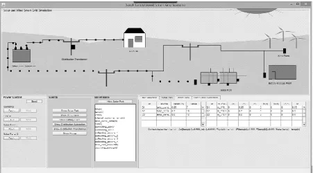
In the customized environment class, there is a GUI showing the entire smart grid scenario (as shown in Figure 3). All six agents have control over their own area and are connected through power lines that distribute electric power from one location to another until it reaches the consumer. The belief base of each agent is shown in the belief base panel (located on bottom panel). The user selects from a choice of buttons which agent’s belief base to display at any one time. The environment also receives input from the buttons on the power control panel (located on bottom panel). Here, the user can introduce a fault into a component within an agent so that it can react to this type of event e.g. introduce a fault within the combiner of the solar park agent. This helps to stimulate the real faults that may occur and ensures the appropriate actions are taken for e.g. recovery, stopping a component etc. The user selection (sensor information) panel (located on the bottom panel) contains a number of sensors for each agent in a user selection tab. The user can select the number of sensors it would like for an agent before generating the smart grid and a number of tabs, each relating to an agent. Each tab contains two tables. The first table shows all the sources evidence i.e. source id, source type, reliability and value. The second table shows the evidence propagated mass function that has been obtained based on the evidential mappings held within the system. In Figure 3, it shows the solar park agent handles three temperature sensors. As the value of temperature changes this will update the mass functions in the second table, thus updating the result of the context-dependent combination rule if the conditions stated in Section 5 have been met. Below these tables, the result of both the context-dependent combination rule and its resulting pignistic probability distribution is stated, alongside the single result used for deriving the belief atom. For example, the frequency is

normal therefore a belief atom temp(n) is inserted into the belief base (as shown in Figure 3).

6.1 Testing Scenarios

The following behaviours can be seen within the implementation to replicate the behaviour of a real-life smart grid.

7

Assume the solar park is working in a normal state. A cyber-attack (tampering sensor information from frequency sources) has caused a number of sensors to record outside of their acceptable ranges for normal operation. As a result, the context-dependent combination rule has been executed and a new belief atom has been derived and used to revise its belief base. The solar park will cease to generate and distribute electric power until the issue has been resolved. The wind farm can instead generate and distribute electric power to the grid (as shown in Figure 4).

Figure 4. The smart grid scenario acquiring power from the wind farm.

The sensors will continually update temperature measurements and the context-dependent combination rule will execute when required on a set of compatible mass functions. The belief base will be revised accordingly when a newly derived belief atom differs from that currently held.

For the solar park agent, we assume that sensor measurements relating to solar panel temperature, internal combiner temperature, frequency, voltage and current are being combined and their corresponding belief atoms are inserted into the belief base (i.e. solar_panel_temp(n), internal_combiner_temp(n), volt(n), freq(n) and

curr(n) respectively).

7. Related Work

In the literature, several approaches consider uncertainty modelling and reasoning within a BDI multi-agent setting. In [14], an agent collects (uncertain) percepts which are fed into a probabilistic graphical model (PGM). An agent’s epistemic state is revised after uncertainty propagation. The classical belief base is revised with belief atoms derived from using a threshold. In [15], the authors use the BDI architecture CanPlan to consider an uncertain belief base where an agent reasons about uncertainty on its own. Specifically, the beliefs of an agent are modelled as a set of epistemic states with a Global Uncertain Belief Set (GUB) allowing the agent to reason about different forms of uncertainty. Contrary to those approaches, our work focuses on modelling and combining uncertain sensor information which is not considered in [14,15]. Furthermore, our work addresses the problem of handling multiple sources of (possibly heterogeneous) information which are often describing the same subject, i.e. different viewpoints. In [15], the authors solely model and reason about uncertain beliefs.

8. Conclusion

8

when to use Dempster's rule of combination and when to resort to Dubois and Prade's disjunctive rule). An AgentSpeak belief atom is then derived to revise the belief base of the agent. In conclusion, we have found it is important to model and combine uncertain sensor information correctly to reflect the true state of the environment as this aids decision making as appropriate plans can be selected. Not only is this work advantageous to the smart grid SCADA system, it can be similarly applied to other SCADA applications dealing with uncertain sensor information and needing to reach a meaningful conclusion.

References

[1] S. Boyer, “SCADA: supervisory control and data acquisition,” International Society Of Automation, 2009.

[2] N. Arghira, D. Hossu, I. Fagarasan, S.S. Iliesc and D.R. Costianu, “Modern SCADA philosophy in power system operation – A survey” UPB Scientific Bulletin, Series C: Electrical Engineering, 73(2):153-166, 2011.

[3] C. Daneels and W. Salter, “What is SCADA?”, In

Proceedings of the 7th International Confererence on Accelator and Large Experimental Physical Control Systems, pages 339-343, 1999.

[4] G. Shafer, “A mathematical theory of evidence,” Princeton University Press, 1976.

[5] J. Ma, W. Liu and P. Miller, “Event modelling and

reasoning with uncertain information for distributed sensor networks” In Proceedings of the 4th International Conference on Scalable Uncertainty Management, pages 236-249, 2010.

[6] A. Hunter and W. Liu, “A context-dependent

algorithm for merging uncertain information in possibility theory,” IEEE Transactions On Systems, Man and Cybernetics, vol. 38, no. 6, pp 1385-1397, 2008.

[7] D. Dubois and H. Prade, “On the combination of evidence in various mathematical frameworks,” Reliability data collection and analysis, pp. 213-241, 1992.

[8] M. Bratman, “Intention, plans and practical reason,”

Harvard University Press, 1987.

[9] A.S. Rao, “AgentSpeak(L): BDI agents speak out in a

logical computable language” In Proceedings of the 7th European Workshop on Modelling Autonomous Agents in a Multi-Agent World, pages 42-55, 1996.

[10] R.H. Bordini, J.F. Hübner and M. Wooldridge, “Programming multi-agent systems in AgentSpeak using Jason”, volume 8, John Wiley & Sons, 2007.

[11] P. Smets, “Decision making in the TBM: the

necessity of the pignistic transformation” International Journal on Approximate Reasoning, 38(2):133-147, 2005.

[12] W. Liu, J. Hughes and M. McTear, “Representing

heuristic knowledge in DS theory” In Proceedings of the 8th International Conference on Uncertainty in Artificial Intelligence, pages 182-190, 1992.

[13] S. Calderwood, K. Bauters, W. Liu and J. Hong, “Adaptive uncertain information fusion to enhance plan selection in BDI agent systems” In Proceedings of the 4th International Workshop on Combinations of Intelligent Methods and Applications, 2014.

[14] Y. Chen, J. Hong, W. Liu, L. Godo, C. Sierra, “Incorporating PGMs into a BDI architecture” In Proceedings of the 16th International Conference on Principles and Practice of Multi-Agent Systems, 2013.

[15] K. Bauters, W. Liu, J. Hong, C. Sierra, “Can(Plan)+: Extending the Operational Semantics of the BDI Architecture to deal with Uncertain Information”, In Proceedings of the 30th International Conference on Uncertainty in Artifical Intelligence, 2014.

Acknowledgements

This work has been funded by EPSRC PACES project (Ref: EP/J012149/1).

Appendix

A. Selection of agent plans

The following plans are continued from those given for the solar park agent in Section 6.

P5: +!run_solar_panel_2 : temp(n) ← collect_protons_2; !run_combiner; …

P6: +!run_combiner : temp(n) & internal_combiner_temp(n) & collecting_protons_1 & collecting_protons_2 ← !run_inverter; combine_input; …

P7: +!run_inverter : temp(n) & freq(n) & combining_input ← convert_power; supply_power;

P8: +!stop_combiner : temp(h) & internal_combiner_temp(h) & not supplying_power ← !maintain_combiner;… P9: +!maintain_combiner: temp(h) & stopped_combiner ← replace_wires; calibrate_combiner;…

P10: +! stop_inverter : temp(h) & internal_inverter_temp(h) & not supplying_grid ← !maintain_inverter;…

P11: +maintain_inverter : temp(h) & internal_inverter_temp(h) & stopped_inverter ← replace_inverter; calibrate_inverter;…

P12: +! freq(l) : collecting_protons_1 & collecting_protons_2 combining_input & converting_power & supplying_power ← !run_wind_farm;…

P13: +!generate_alert : freq(l) | freq(h) ← send_message; sound_alarm;…

9

P15: +fault_solar_panel_1: not collecting_protons_1 & not solar_panel_temp(n) ← maintain_solar_panel_1;…

Agent: Distribution Substation

Assume the distribution substation consists of two step-down transformers with one being used as a replacement when needed, two incoming power cables and sensors measuring incoming and outgoing voltage, internal substation and internal transformer temperature, incoming and outgoing frequency.

P16: +!prepare_to_start_distribution_substation : true ← calibrate_step_down_transformer_1; !start_distribution_substation;…

P17: +!start_distribution_substation: not distributing_low_volt_power & not obtaining_high_tran_power & calibrated_step_down_transformer_1 ← !run_step_down_transformer_1;…

P18: +!run_step_down_transformer_1 : internal_substation_temp(n) & internal_transformer_temp(n) & incoming_volt(n) & outgoing_volt(n) & obtaining_high_tran_power ← step_down_power; distribute_low_volt_power;…

P19: +internal_substation_temp(h) : step_down_power & internal_transformer_temp(n) ← switch_off_heater; switch_on_air_con;…

P20: +internal_substation_temp(l) : step_down_power & internal_transformer_temp(n) ← switch_on_heater; switch_off_air_con;…

P21: +fault_cable_1 : true ← disconnect_cable_1; connect_cable_2; !maintain_cable_1;…;

P22: +!maintain_cable_1 : disconnected_cable_1 ← replace_cable_1;

P23: +internal_transformer_temp(h) : not stepping_down_power & incoming_volt(n) ← !stop_step_down_transformer_1;

calibrate_step_down_transformer_2; !run_step_down_transformer_2

P24: +!run_step_down_transformer_2 : calibrated_step_down_transformer_2 & obtaining_high_tran_power ← step_down_power; distribute_low_volt_power;…

P25: +! stop_step_down_transformer_1 : internal_transformer_temp(h) & not stepping_down_power ← !maintain_step_down_transformer_1;…

P26: +!maintain_step_down_transformer_1 : stopped_step_down_transformer_1 ←

replace_internal_component;

calibrate_step_down_transformer_1;…

P27: +fault_cable_1 : wind(h) ← disconnect_cable_1; connect_cable_2; !maintain_cable_1;…

Agent: Distribution Transformer

Assume the distribution transformer consists of sensors measuring incoming and outgoing voltage, internal transformer temperature, incoming and outgoing frequency, oil absorbance.

P28: +!prepare_to_start_distribution_transformer : true ← calibrate_transformer; !start_distribution_transformer;…

P29: +!start_distribution_substation: not distributing_lower_volt_power & not obtaining_high_dist_power & calibrated_transformer ← !run_transformer;… P30: +!run_step_down_transformer : internal_transformer_temp(n) _oil-absorbance(n) & incoming_volt(n) & outgoing_volt(n) & obtaining_high_dist_power ← reduce_power; distribute_lower_volt_power;…

P31: +oil_absorbance(h) : reducing_power ← replace_transformer;…

Agent: Wind Farm

Assume the wind farm contains three wind mills where the wind will turn the rotor blades. The blade will then turn a shaft inside the nacelle which is attached to a gearbox to increase rotation speed. The generator converts rotational energy to electrical energy for transmission to the grid. Sensors will measure wind speed and direction.

P32: +!prepare_to_start_wind_farm : true ← calibrate_generator_1; calibrate_generator_2; calibrate_generator_3; !start_wind_farm.

P33: +!start_wind_farm : not supplying_grid & calibrated_generator_1 & calibrated_generator_2 & calibrated_generator_3 ← !run_wind_mill_1; !run_wind_mill_2, !run_wind_mill_3;…

P34: +!run_wind_mill_1 : wind_speed(n) wind_direction(n) ← move_blades_1; !run_nacelle_1; rotate_tower_head_1(90);… P35: +!run_wind_mill_2 : wind_speed(n) wind_direction(n) ← move_blades_2; !run_nacelle_2; rotate_tower_head_2(45);… P36: +!run_wind_mill_3 : wind_speed(n) wind_direction(n) ← move_blades_3; !run_nacelle_3; rotate_tower_head_3(180);…

10

P38: +!run_nacelle2 : moving_blades_2 ← !run_gearbox_2; turns_shaft_2;…

P39: +!run_nacelle_3 : moving_blades_3 ← !run_gearbox_3; turns_shaft_3;…

P40: +!run_gearbox_1 : turning_shaft_1 ← !run_generator_1; increase_rotation_speed_1;…

P41: +!run_gearbox_2 : turning_shaft_2 ← !run_generator_1; increase_rotation_speed_2;… P42: +!run_gearbox_3 : turning_shaft_3 ← !run_generator_3; increase_rotation_speed_3;… P43: +!run_generator_1 : increased_rotation_speed_1 ← convert_rotational_power_1; supply_grid;… P44: +!run_generator_2 : increased_rotation_speed_2 ← convert_rotational_power_2; supply_grid;…

P45: +!run_generator_2 : increased_rotation_speed_2 ← convert_rotational_power_2; supply_grid;…

P46: +wind_speed(l) : not supplying_grid ← !stop_wind_mill_1; !stop_wind_mill_2, !stop_wind_mill_3; !run_solar_park; !run_battery_storage;…

P47: +fault_blade_1: wind_speed(h) & wind_direction(h) ← !stop_wind_mill_1; rotate_tower_head_2; rotate_tower_head_3;…

Agent: House

Assume the house is a grid-connected residential solar PV system that consists of a solar panel, an inverter and a meter (measuring electric power production and consumption). Sensors will measure temperature, voltage and frequency.

P48: +!prepare_to_start_house_ : true ← calibrate_inverter; calibrate_meter; !start_house.

P49: +!start_house : not supplying_grid & calibrated_inverter & calibrated_meter ← !run_solar_panel_1;…

P50: +!run_solar_panel_1 : temp(n) ← collect_protons; !run_inverter; …

P51: +!run_inverter: temp(n) & freq(n) & volt(n) & collecting_protons ← convert_power; !run_meter;…

P52: +!run_meter: temp(n) & freq(n) & volt(n) & converting_power ← measure_usage; use_appliance;…;

P53: +fault_meter : not measuring_usage ← !generate_alert;…;

P54: +volt(h) : collecting_protons & converting_power & using_appliance ← supply_grid;…

P55: +volt(l) : collecting_protons & converting_power & not using_appliance ← obtain_power_from_grid,…

P56: +fault_inverter : collecting_protons & not converting_power ← !generate_alert; !stop_inverter; obtain_power_from_grid;…

P57: +!stop_inverter : ← temp(h) & not converting_power & not supplying_grid ← !maintain_inverter;…

P58: +generate_alert : not measuring usage | not converting_power ← send_message_home_owner; flash_light_on_meter; send_message_utility;… P59: +maintain_inverter : temp(h) & stopped_inverter ← replace_inverter; calibrate_inverter;…