Information Fusion for Pattern Classification in Complex Interconnected Systems

University of Connecticut

OpenCommons@UConn

Doctoral Dissertations University of Connecticut Graduate School

1-19-2016

Information Fusion for Pattern Classification in

Complex Interconnected Systems

Nayeff Najjar

[email protected]

Follow this and additional works at:https://opencommons.uconn.edu/dissertations

Recommended Citation

Najjar, Nayeff, "Information Fusion for Pattern Classification in Complex Interconnected Systems" (2016).Doctoral Dissertations. 1334.

Information Fusion for Pattern Classification in

Complex Interconnected Systems

Nayeff Najjar, PhD University of Connecticut 2017

Typical complex interconnected systems consist of several interconnected components with several heterogeneous sensors. Classification problems (e.g., fault diagnosis) in these systems are chal-lenging because sensor data might be of high dimension and/or convey misleading or incomplete information. So, this thesis performs optimal sensor selection and fusion to lower computational complexity and improve classification accuracy.

First, the thesis presents the novelUnsupervised Embeddedalgorithm for optimal sensor selection. The algorithm uses the minimum Redundancy Maximum Relevance (mRMR) criterion to select the candidate list of sensors, then usesK-means clustering algorithm and entropy criterion to select the optimal sensors. The Unsupervised Embedded algorithm is applied to heat exchanger fouling severity level diagnosis in an aircraft.

Second, the thesis presents a fusion algorithm for classification improvement called the

Better-than-the-Best Fusion (BB-Fuse) algorithm, which is analytically proven to outperform the best

sensor Correct Classification Rate (CCR). Using confusion matrices of individual sensors, the BB-Fuse selects the optimal sensor-class pairs and organizes them in a tree structure where one class is isolated at each node. The BB-Fuse algorithm was tested on two human activity recognition data sets and showed CCR improvement as expected.

Using the confusion matrices is a limitation of the BB-Fuse algorithm because of high computa-tion complexity and pertinence to specific classifiers. So, the thesis next presents theDecomposed

Sensor-Class Pair Tree with maximum Admissible-Relevance for Fusion (D∗-Fuse) algorithm,

which is a novel sensor-class pair selection and fusion algorithm. Instead of using the confusion matrices, the D∗-Fuse algorithm uses a novel classifier-independent information-theoretic crite-rion (i.e., Admissible-Relevance (AR) criterion) to obtain the sensor-class pair. As a result, any classifiers can be used with the D∗-Fuse Tree.

In comparison to other sensor selection algorithms in literature, the novel AR criterion has two major advantages. First, the AR criterion ensures selection of non-redundant sensors by selecting optimal sensor-class pairs. This pair selection ensures that the selected sensors carry signatures about different classes; i.e., they convey non-redundant classification information. Second, the AR criterion outputs a general fusion tree that suggests an order in which the sensors should be used.

Information Fusion for Pattern Classification in

Complex Interconnected Systems

Nayeff Najjar

B.S., King Fahd University of Petroleum and Minerals, 2005 M.S., Widener University, 2008

M.S., University of Connecticut, 2016

A Dissertation

Submitted in Partial Fullfilment of the Requirements for the Degree of

Doctor of Philosophy at the

University of Connecticut

Copyright by

Nayeff Najjar

Approval Page

Information Fusion for Pattern Classification in

Complex Interconnected Systems

Presented by Nayeff Najjar

Major Advisor

Prof. Shalabh Gupta

Associate Advisor

Prof. Peter Luh

Associate Advisor

Prof. Rajeev Bansal

University of Connecticut 2017

Acknowledgments

I would like first to express my appreciations to the highness of King Abdullah bin Abdulaziz (RIP), the previous king of Saudi Arabia. King Abduallah initiates a scholarship program through which thousands of Saudi students have the opportunity to join top universities worldwide and; especially the United States of America. I been lucky to gain on of these scholarships using which I continued my higher education and for that I feel grateful.

Next, I would like to thank my advisor, Dr. Shalabh Gupta. Dr. Gupta’s mentoring through my PhD work helped me to improve my academic skills. In his lab, he encouraged teamwork and gave me the opportunity to improve my leadership and communication skills. It was not possible to develop my PhD theory without his kind directions and advice. Thank you Dr. Gupta.

Besides that, I would like to express my gratitude to my mother, Thuraiyah Najjar, and father, Abdularahman Najjar, for all encouragements and support. My mother was my first teacher and her contribution to my personality is invaluable and so was my father.

Through my life, many of family members and friends have been generous with encouragements, kind wishes and advices. I would like to seize this opportunity to thank all of them; especially, my father in law, Jameel Itraji and my uncle, Ghazi Najjar.

Last but not least, I would like to thank my wife, Israa Itraji. The years I spent in my PhD work were hard and time consuming. Her patience and persistent support were vital for me to be successful in my PhD.

TABLE OF CONTENTS

List of Figures x

List of Tables xii

Chapter 1: Introduction 1

1.1 Background and Motivation . . . 1

1.2 Outline and Contributions . . . 2

1.3 List of Publications . . . 4

Chapter 2: Unsupervised Embedded Sensor Selection for Classification Algorithm 6 2.1 Introduction . . . 6

2.1.1 Application . . . 7

2.1.2 Approach and Contributions . . . 9

2.2 Literature Review . . . 11

2.2.1 Sensor Selection Algorithms . . . 11

2.2.2 Fault Diagnosis Algorithms . . . 11

2.3 System Description . . . 12

2.3.1 Primary and Secondary Heat Exchangers . . . 13

2.3.3 Heat Exchanger Fouling Diagnosis Architecture . . . 19

2.4 Optimal Sensor Selection Methodology . . . 19

2.4.1 Information-theoretic Measures . . . 21

2.4.2 Data Partitioning for Symbol Sequence Generation . . . 22

2.4.3 minimum Redundancy Maximum Relevance (mRMR) . . . 24

2.4.4 Embedded Algorithm . . . 27

2.4.5 Unsupervised Embedded Algorithm . . . 27

2.5 Data Analysis for Fouling Diagnosis . . . 28

2.5.1 Feature Extraction . . . 29

2.5.2 Classification . . . 30

2.5.3 Sensor Fusion . . . 31

2.6 Results and Discussion . . . 31

2.7 Conclusions . . . 36

Chapter 3: BB-Fuse: Optimal Sensor-Class Pair Selection and Fusion Algorithm for Classification 39 3.1 Introduction . . . 39

3.2 Literature Review . . . 41

3.2.1 Voting Methods . . . 41

3.2.2 Bayesian Fusion Methods . . . 42

3.2.3 Boosting Methods . . . 43

3.2.4 Decision Tree Methods . . . 43

3.3 Mathematical Preliminaries . . . 44

3.4 BB-Fuse Algorithm . . . 46

3.4.1 Objective . . . 46

3.4.2 BB-Fuse Training Phase . . . 47

3.4.3 BB-Fuse Testing Phase . . . 52

3.5.1 BB-Fuse Optimality . . . 52

3.5.2 BB-Fuse Complexity . . . 60

3.6 Results and Discussion . . . 61

3.6.1 Application I: Human Activity Recognition . . . 61

3.6.2 Application II: User Identification . . . 65

3.7 Conclusions . . . 67

Chapter 4: D∗-Fuse: Optimal Sensor-Class Pair Selection and Fusion Algorithm for Classification 70 4.1 Introduction . . . 70

4.1.1 Basics of Information Theory . . . 72

4.2 Literature Review . . . 74

4.2.1 MD Criterion . . . 74

4.2.2 MR Criterion . . . 76

4.3 D∗-Fuse Algorithm . . . 78

4.3.1 Objectives . . . 78

4.3.2 D∗-Fuse Training Phase . . . 79

4.3.3 D∗-Fuse Testing Phase . . . 84

4.4 Results and Discussion . . . 84

4.4.1 Application I: Simulated Data . . . 84

4.4.2 Application II: Gesture Phase Segmentation . . . 88

4.4.3 Application III: Human Activity Recognition Dataset . . . 92

4.5 Conclusions . . . 96

Chapter 5: Conclusions 98 5.1 Unsupervised Embedded Algorithm . . . 98

5.2 BB-Fuse Algorithm . . . 100

Appendix A: Matters Relevant to Information Theory 104

A.1 Maximum Entropy Distribution . . . 104

A.2 Calculation of Mutual Information . . . 105

A.3 Fano’s Inequality . . . 106

Appendix B: Machine Learning Algorithms 108 B.1 Principal Component Analysis (PCA) . . . 109

B.2 Linear Discriminant Analysis . . . 109

B.3 k-Nearest Neighbor Classification Algorithm . . . 110

Appendix C: Fusion Algorithms 112 C.1 CaRT and C4.5 . . . 112

C.2 Bayes Belief Integration . . . 114

C.3 Majority Voting . . . 115

C.4 Adaptive Boosting . . . 116

C.5 Borda Count Voting . . . 117

C.6 Condorcet Count Voting . . . 118

LIST OF FIGURES

1.1 Research Themes Summary and Connections . . . 4

2.1 Environmental Control System (ECS) Schematics . . . 8

2.2 An Illustration of the Plate Fin Heat Exchanger . . . 9

2.3 Heat Exchanger Fouling Diagnosis Algorithm whered= 1,2. . .5 . . . 10

2.4 Normalized Flow vs Secondary Heat Exchanger Impedance . . . 14

2.5 Stochastic time series data of three critical sensors for five different day types . . . 17

2.6 An illustration of the Maximum Entropy Partitioning . . . 25

2.7 An example of using the K-means clustering algorithm and the entropy criterion to rank sensors . . . 28

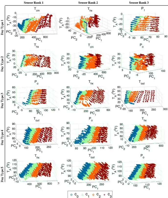
2.8 Top three unsupervised embedded optimal sensors’ principal components 1 and 2 vs the ambient temperature for day types1,2, . . .5 . . . 34

3.1 Decision Tree Types;

C

3.2 An Illustration of the Grafting and Node Merging Operations on One-vs-the-Rest Trees; where

C

3.3 The Structure of a BB-Fuse Tree (

T

3.4 An Example of the BB-Fuse Tree Construction . . . 51

3.6 Placement of (a) Inertial Measurement Units (IMUs), (b) Subject Acceleration Devices, (c) Reed Sensors and (d) Object Acceleration Devices in Application I

Dataset [116, 117] . . . 62

3.7 The BB-Fuse Tree for Application I. . . 64

3.8 Thex, yandz axes for the Android Phones. . . 66

3.9 The BB-Fuse Tree for Application II. . . 67

4.1 EntropyH(C), Conditional EntropyH(C|S)and Mutual InformationI(C;S). . . 74

4.2 Venn Diagrams for Maximum Dependency (MD) and Maximum Relevance (MR) criteria . . . 75

4.3 D∗-Fuse Tree

T

4.4 Admissible Relevance (AR) Venn Diagram . . . 80

4.5 D∗-Fuse Tree for Application I . . . 85

4.6 Sample Means and Variances for the Simulated Data . . . 86

4.7 The4main Gesture Phases [122]. The Hold Phase is not shown and it is simply a pause before or after the Stroke Phase. . . 89

4.8 D*-Fuse Tree for Application II . . . 90

4.9 2ndOrder Gaussian Mother Wavelet . . . 93

LIST OF TABLES

2.1 List of Critical Sensors in the ECS . . . 8

2.2 Input Parameters and Fouling Classes . . . 18

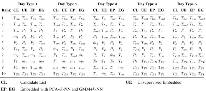
2.3 Decreasingly Sorted Candidate List and Optimal Sensor Sets . . . 32

2.4 Confusion Matrices of the Optimal Sensors with PCA +k-NN for Classification . . 35

2.5 Confusion Matrices for the Optimal Sensors with GMM +k-NN for Classification 36 2.6 Classification Results for the Top Three Optimal Sensors Obtained using the UE Algorithm . . . 37

2.7 Computation Time for Various Procedures Used for Heat Exchanger Fouling Di-agnosis . . . 38

3.1 Description of Sensing Devices, Modalities, and Locations for Application I Dataset 63 3.2 Application I: Confusion Matrices for Different Methods . . . 64

3.3 Application I: Description of the Optimal Sensors . . . 64

3.4 Application I: CCRs for Different Methods . . . 65

3.5 Application I: Execution Times . . . 65

3.6 Application II: Description of the Optimal Sensors. . . 67

3.7 Confusion Matrices for the User Identification from Walking Activity Dataset . . . 68

3.8 Application II: CCRs for Different Methods . . . 68

4.1 Sensor Data Distribution for Application I . . . 85

4.2 Optimal Sensors and CCRs for Application I . . . 85

4.3 Confusion Matrices for Application I . . . 87

4.4 Sensor Definition . . . 89

4.5 Optimal Sensors and CCRs for Application II . . . 90

4.6 Confusion Matrices for Application II . . . 91

4.7 Class and Sensor Set Definition for Application III . . . 92

4.8 Optimal Sensor Sets for Application III . . . 94

4.9 Confusion Matrices for Application III . . . 95

4.10 CCRs for Various Sensor Selection and Fusion Algorithms for the Human Activity Recognition Dataset . . . 96

CHAPTER

1

INTRODUCTION

1.1

Background and Motivation

Classification problems arise in a plethora of modern applications including security, entertain-ment, surveillance, medical, engineering, geoscience and many other applications [1–9]. Most modern systems (e.g., aerospace, automobile and robotic systems) can be described as complex interconnected systems, where the components are interconnected via electrical, mechanical or wireless connections. Typically, several heterogeneous sensors are scattered all over these systems for monitoring and control purposes (e.g., fault diagnosis and prognosis, activity recognition and situation awareness). Accurate classification could be challenging in these systems due to various types of complexities including data, operational, and system complexities. First of all, the data could be complex because of the multitude of heterogeneous sensors which makes the analysis computationally expensive. Second, operational complexity stems from the fact that the system response may vary with respect to ambient conditions; in turn, class signatures vary from one ambient condition to another which may confuse the classifiers. Last but not the least, system complexity is due to the interconnections between the components; as a result, sensors may carry redundant, misleading or complementary classification information.

obtaining a unified, robust and reliable classification decision using information fusion techniques. In this regard, there are three themes in this thesis as introduced next where the details are in Chapters 2,3 and 4.

1.2

Outline and Contributions

The first theme addresses the problem of optimal sensor set selection with application to heat exchanger fouling diagnosis in the Environmental Control System (ECS) of an aircraft. The ECS is a complex interconnected system that controls the temperature, humidity level and pressure of the cabin air of an aircraft. One of the major components in the ECS is the heat exchanger which exchanges the heat with the ram air. The heat exchanger is prone to the fouling phenomenon, which is the accumulation of debris on the surface of the heat exchanger. Fouling reduces the efficiency of the heat exchanger, might occur unexpectedly and may lead to cascading failures of other expensive components. Subsequently, it is required to perform periodic maintenance of the heat exchanger. Unfortunately, this maintenance incurs high financial and time costs. This motivates the design of an automated heat exchanger fouling diagnosis algorithm.

Heat exchanger fouling diagnosis is challenging because the ECS sensor readings vary with respect to ambient temperatures and altitudes of airports across the world. Furthermore, the ECS is prone to various sources of uncertainties such as measurement noises and vibrations. Moreover, fouling diagnosis is difficult and computationally expensive due to the large number of hetero-geneous sensors. So, the thesis presents theUnsupervised Embedded sensor selection algorithm, which is an automated method that selects optimal, non-redundant sensor set for data reduction and reliable fouling diagnosis.

This algorithm is of two steps. In the first step, the algorithm uses the popular

minimum-Redundancy-Maximum-Relevance(mRMR) [10] algorithm to select a candidate list of sensors. In

the second step, the algorithm uses K-means clustering algorithm to cluster the data, and then ranks the sensors based on the average entropy of the clusters of each sensor.

Rate (CCR). Most information fusion algorithms that are available in literature lack the analytical guarantee of CCR improvement. This thesis presents a novel algorithm called the

Better-than-the-Best Fusion(BB-Fuse) algorithm, which is analytically proven to improve the CCR. The BB-Fuse

algorithm exploits the fact that different sensors isolate different classes with different accuracies. Subsequently, the BB-Fuse algorithm uses the confusion matrices that result from different sensors to search for the optimal sensor-class pairs. Finally, the BB-Fuse organizes them in a fusion tree that isolates one class at a time.

The first and the second themes addressed the sensor selection problem and the fusion problem for CCR improvement; however, both of the above algorithms have certain limitations. In regards to the first theme, the Unsupervised Embedded algorithm is computationally efficient and performs better in comparison to existing sensor selection algorithms; however, it relies on the mRMR algorithm which is criticized in literature for subtracting the minimum redundancy criterion [11].

In regards to the second theme, the BB-Fuse algorithm guarantees CCR improvement; however, it relies on the confusion matrices of the sensors. The confusion matrices are not only expensive to compute but also pertain to specific classifiers. In other words, there would be a different optimal fusion tree if different classifiers are used because the optimal sensor-class pairs would differ.

To address the above limitations, the third theme presents the Decomposed Sensor-Class Pair

Tree with maximum Admissible-Relevance for Fusion(D∗-Fuse) algorithm, which is a novel

sensor-class pair set selection and fusion algorithm. Similar to the BB-Fuse, the D∗-Fuse algorithm utilizes the fact that sensors differ in the quality with which they can isolate individual classes. However, the D∗-Fuse algorithm depends on an information-theoretic sensor-class pair selection criterion (called the Admissible Relevance (AR) criterion) instead of the confusion matrices of individual sensors. Subsequently, any set of classifiers can be trained at the nodes of the resultant sensor-class tree structure.

The D∗-Fuse algorithm has two major improvements over the mRMR. First, the D∗-Fuse algo-rithm selects optimal “sensor-class” pair set rather than selecting “sensor” set only. As a result, sensor redundancy between the optimal selected sensors does not exist since the selected sen-sors carry information that isolate different classes. Second, the D∗-Fuse algorithm outputs a tree

Theme 1:

Unsupervised Embedded Algorithm (Optimal Sensor Selection Algorithm)

Theme 2: BB-Fuse Algorithm (Optimal Sensor-Class pair Selection and Fusion Algorithm)

Them 3: D*-Fuse Algorithm (Optimal Sensor-Class pair Selection and Fusion Algorithm)

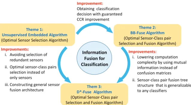
Improvements:

i. Lowering computation complexity by using mutual information instead of confusion matrices

ii. Sensor-class pair fusion tree structure that is generalizable to any classifiers

Improvement:

Obtaining classification decision with guaranteed CCR improvement

Improvements:

i. Avoiding selection of redundant sensors ii. Optimal sensor-class pairs

selection instead of only sensors

iii. Constructing general sensor fusion architecture

BB-Fuse: Better-than-the-Best Fusion

CCR: Correct Classification Rate

D*-Fuse: Decomposed Sensor-Class Pair Tree with Maximum

Admissible-Relevance for Fusion

Information Fusion for Classification

Figure 1.1: Research Themes Summary and Connections

structure to fuse the optimal sensors. Figure 1.1 summarizes the three research themes and the connections between them.

1.3

List of Publications

Journal Papers

1. N. Najjar, S. Gupta, J. Hare, S. Kandil, and R. Walthall, “Optimal sensor selection and fusion for heat ex-changer fouling diagnosis in aerospace systems,”IEEE Sensors Journal, vol. 16, no. 12, pp. 4866–4881, 2016.

2. N. Najjar, C. Sankavaram, J. Hare, S. Gupta, K. Pattipati, R. Walthal, and P. D’Orlando, “Health assess-ment of liquid cooling system in aircrafts: Data visualization, reduction, clustering and classification,”SAE International Journal of Aerospace, vol. 5, no. 1, pp. 119–127, 2012.

3. N. Najjarand S. Gupta, “BB-Fuse: An information fusion algorithm for n-class classification problems,”IEEE Transactions on Pattern Analysis and Machine Intelligence, Submitted.

Conference Papers

4. N. Najjarand S. Gupta, “Better-than-the-Best Fusion algorithm with application in human activity recogni-tion,” in Proceedings of SPIE Multisensor, Multisource Information Fusion: Architectures, Algorithms, and Applications 2015, SPIE, 2015, pp. 949805-1 – 949805-10.

5. N. Najjar, J. Hare, P. D’Orlando, G. Leaper, K. Pattipati, A. Silva, S. Gupta, and R. Walthall, “Heat exchanger fouling diagnosis for an aircraft air-conditioning system,” inProceedings of SAE 2013 AeroTech Congress and Exibition- Technical Paper 2013-01-2250, SAE International, 2013.

6. N. Najjar, C. Sankavaram, J. Hare, S. Gupta, K. Pattipati, R. Walthall, and P. D’Orlando, “Health assessment of liquid cooling system in aircrafts: Data visualization, reduction, clustering and classification,” in Proceed-ings of SAE 2012 Aerospace Electronics and Avionics Systems Conference- Technical Paper 2012-01-2106, SAE International, 2012, pp. 119–127.

7. J. Wilson,N. Najjar, J. Hare, and S. Gupta, “Human activity recognition using lzw-coded probabilistic finite state automata,” inProceedings of 2015 IEEE International Conference on Robotics and Automation (ICRA), IEEE, 2015, pp. 3018–3023.

8. J. Hare, S. Gupta,N. Najjar, P. D’Orlando, and R. Walthall, “System-level fault diagnosis with application to the environmental control system of an aircraft,” in Proceedings of SAE 2015 AeroTech Congress and Exhibition- Technical Paper 2015-01-2583, SAE International, 2015.

9. A. Silva,N. Najjar, S. Gupta, P. D’Orlando, and R. Walthall, “Wavelet-based fouling diagnosis of the heat exchanger in the aircraft environmental control system,” inProceedings of SAE 2015 AeroTech Congress and Exhibition- Technical Paper 2015-01-2582, SAE International, 2015.

Patents

10. N. Najjar, S. Gupta, J. Hare, G. Leaper, P. D’Orlando, R. Walthall, and K. Pattipati,Optimal sensor selection and fusion for heat exchanger fouling diagnosis in aerospace systems, 14/700,769, (Submitted).

11. J. Hare, S. Gupta,N. Najjar, P. D’Orlando, and R. Walthall,System level fault diagnosis for the air manage-ment system of an aircraft, 14/687,112, (Submitted).

12. A. Silva,N. Najjar, S. Gupta, P. D’Orlando, and R. Walthall,Wavelet-based analysis for fouling diagnosis of an aircraft heat exchanger, 14/689,467, (Submitted).

CHAPTER

2

UNSUPERVISED EMBEDDED SENSOR SELECTION FOR

CLASSIFICATION ALGORITHM

2.1

Introduction

Optimal sensor set selection is essential for classification in complex interconnected systems. Pri-marily, optimal sensor set selection reduces the data and in turn computational complexity. Fur-thermore, it increases classification accuracy because some sensors might convey misleading or partial classification information. Optimal sensor set selection can sometimes be counter intu-itive in complex interconnected systems because of direct or feedback interconnections between the components. Hence, automated data-driven optimal sensor selection is desirable in complex interconnected systems.

Recent literature has developed several sensor selection algorithms that are categorized into two main types based on their evaluation criteria. The first in this category are theWrapper Algorithms

that depend on the evaluation of the Correct Classification Rate (CCR)1 _{for each sensor using a}

specified classifier [12–14]. Wrapper algorithms usually lead to a high CCR but are computation-ally expensive if the number of sensors is large because they rely on thecross-validationalgorithm to calculate the CCR. Besides that, the wrapper algorithms cannot be generalized to any classifier.

The second type are theFilter Algorithmsthat evaluate the performance of each sensor based on an evaluation function. Recently, many filter algorithms have been developed using the concepts of information theory [10, 15]. Filter algorithms do not depend on the classifier, are computationally less expensive, and may perform as good as the wrapper algorithms [13].

In addition, there exist the Embedded Algorithmsthat take advantage of both the wrapper and the filter algorithms. The embedded algorithms use a filter to select a candidate list of sensors and then apply a wrapper on this list to rank the optimal sensor set [10]. Embedded algorithms are less expensive than wrappers and more accurate than filters; yet they are pertinent to the specified classifier [16]. Several search methods have been suggested for the above algorithms, such as the forward and backward search [10, 15]. Dash and Liu [17] compared different such search methods. This theme presents a modified embedded sensor selection algorithm which is called the Un-supervised Embedded algorithm. The first step of the algorithm usesminimum Redundancy

Max-imum Relevance (mRMR) criterion [10] as a filter to initiate a candidate list. Subsequently, the

second step of the algorithm is clustering based sensor ranking, which relies onK-means clus-tering method instead of a specific classifier to rank the sensors in the candidate list. This method has low computational complexity, faster execution, and it does not depend on a specific classifier. Once the optimal set of sensors is selected, different machine learning tools can be applied for data analysis and fusion to make classification decisions.

2.1.1 Application

For applicatin, this theme uses theEnvironmental Control System (ECS) of an aircraft as an ex-ample of a complex interconnected system. The ECS is a system which regulates temperature, pressure and humidity of the cabin air of an aircraft. The ECS consists of various components such as the primary and secondary heat exchangers, turbines, compressor, condenser, and water extractor as schematically shown in Fig. 2.1 where the sensros are defined in Table 2.1. These components are interconnected through various mechanical and pneumatic connections. In addi-tion, various sensing devices (more than 100 parameter recorded) such as temperature, pressure and flow sensors are mounted at different locations in the ECS [18, 19].

Figure 2.1:Environmental Control System (ECS) Schematics Table 2.1:List of Critical Sensors in the ECS

S Description S Description

˙

m1 PD mass flow rate m˙2 SD mass flow rate

T1 PD air temperature T2 SD air temperature

P1 PD air pressure P2 SD air pressure

Pi SHX input pressure Po SHX output pressure

Thx SHX output temperature TcmCompressor output temperature ToutECS output temperature Tcn Condenser output temperature TF DFlight deck zone temperature TZjZoneZj∀j= 1. . . nztemperature

S: Sensor SHX: Secondary heat exchanger PD: Primary bleed air duct SD: Secondary bleed air duct

nz: The number of zones in the cabin

Heat exchangers are critical components of the ECS of an aircraft. Typically, several plate fin heat exchangers are used in an ECS, which consist of plates and fins stacked over each other as shown in Fig. 2.2. Plate fin heat exchangers are used in this application because of their compact design, light weight and high efficiency. Often, physical objects (e.g., debris) accumulate on the fins of the heat exchanger due to particulates and other contaminants present in the air stream. This phenomenon is known asfoulingwhich obstructs the flow of the cooling medium through the heat exchanger and hence degrades its efficiency.

In absence of an automated fouling diagnosis methodology, heat exchanger necessitates peri-odic and expensive maintenance [20]. On top of maintenance costs, fouling diagnosis incurs fi-nancial losses that result from the aircraft flight interruption that last several days. Besides, fouling may occur unexpectedly and, in extreme cases, can lead to damage of other expensive components (i.e., cascading failures). As such, early fouling diagnosis is of utmost importance to facilitate

Condition Based Maintenance(CBM)2 _{and to avoid cascading failures.}

2.1.2 Approach and Contributions

A high fidelity ECS Simulink model that is provided by our industry partner was used for data generation. To reduce system modeling uncertainty, the Simulink model was validated using actual flight test data operating under nominal conditions. System validation is an iterative process in which actual flight data is compared with Simulink output data; after that, the Simulink model is tuned to minimize the residuals. Next, the Simulink model output data is compared with actual flight data again and so on. The process terminates when the residuals are within acceptable tolerance.

The Simulink model inputs include the ambient temperature, altitude, occupant count and air-craft state (on-ground or flying). In addition, heat exchanger fouling condition can be injected into

Figure 2.2: An Illustration of the Plate Fin Heat Exchanger 2_{Condition Based Maintenance (CBM) is to perform maintenance only when necessary}

Parametric Combinations of OCC & Ambient Temperature Various

Fouling Conditions

Simulink Model

Training Data Set of m_sensors

Optimal Sensor Selection

Data from Optimal Sensors ݏ_ଵכ,ݏ_ଶכand ݏ_ଷכ Optimal Sensors ݏଵכ,ݏଶכand ݏଷכ Feature Extraction ݏଵכFeatures ݏଶכFeatures ݏଷכFeatures

Training Phase for Day Type ݀

׊ ݀=1, 2, 3, 4, 5

OCC & Ambient Temperature Unknown Fouling Condition c Unlabeled Data of m_sensors Pick Optimal Sensors’ Data

Data from Optimal Sensors ݏ_ଵכ,ݏ_ଶכand ݏ_ଷכ

Feature Extraction

Testing Phase for Day Type _݀

׊ ݀=1, 2, 3, 4, 5 Classifier Training Classifier 1 Classifier 2 Classifier 3 ݏଵכFeatures ݏଶכFeatures ݏଷכFeatures Majority Vote Fusion Ƹܿ ଵ Ƹܿ ଶ Ƹܿ ଷ Ƹܿ Enhanced Decision Classifier 1 Classifier 2 Classifier 3 Simulink Model

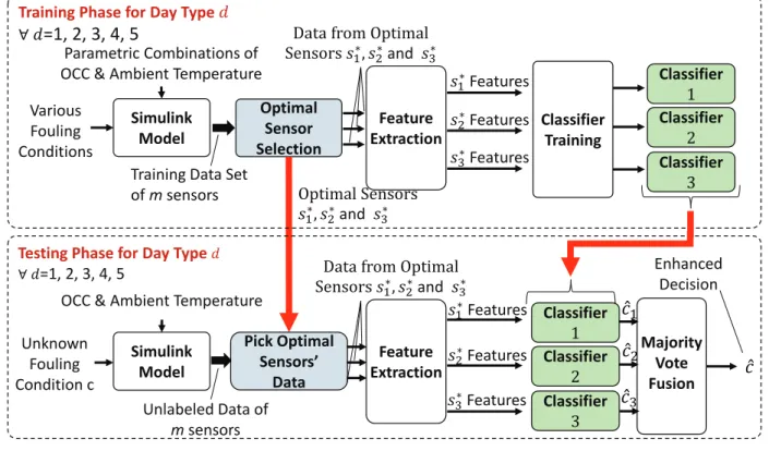
Figure 2.3: Heat Exchanger Fouling Diagnosis Algorithm whered= 1,2. . .5

the Simulink model by varying the flow impedance through the heat exchanger. The Simulink model outputs time series data of more than 100 sensor parameters.

To accommodate the system behavior under various input conditions, the ambient temperatures and passenger loads are tabulated as discussed in the Section 2.3.2. After that, fouling classes are defined based on the air-flow through the heat exchanger. Then, the validated Simulink model of the ECS is used to generate sensor data for nominal and different fouling conditions of the heat exchanger while considering various sources of uncertainties in the system. After data generation, machine learning algorithms are applied to obtain a fouling decision. The heat exchanger fouling diagnosis algorithm is shown in Fig. 2.3.

The main contributions are below:

• Optimal sensor set selection for fouling diagnosis using a novel Unsupervised Embedded

Algorithm, that uses the mRMR criteria as a filter and the K-means clustering method for

ranking.

distributions and to estimate the mutual information in the mRMR criteria.

2.2

Literature Review

2.2.1 Sensor Selection Algorithms

Sensor/feature selection for classification has gained interest in literature. Han et al. [21] studied feature selection problem for chillers. Namburu et al. [22] used genetic algorithm for sensor se-lection and applied SVM, PCA, and Partial Least Squares (PLS) for fault classification in HVAC systems. Optimal sensor selection for discrete-event systems with partial observations was per-formed by Jiang and Kumar [23]. Gupta et al. [24] discussed stochastic sensor selection with application to scheduling and sensor coverage. Joshi and Boyd [25] used convex optimizationto perform sensor selection. Hero and Cochran [26] provided a review of the methods and applica-tions of sensors management. Xu et al. [27] used sensor configuration, usage and reliability costs for sensor selection for PHM of aircraft engines. Shen, Liu and Varshney [28] considered the problem of multistage look-ahead sensor selection for nonlinear dynamic systems.

2.2.2 Fault Diagnosis Algorithms

Several techniques have been proposed in recent literature for fault detection, diagnosis and prog-nosis (FDDP) of air-conditioning systems, in particular,Heating, Ventilating and Air Conditioning

(HVAC) systems [29–31]. Katipamula and Brambley introduced a two-part survey of FDDP of HVAC systems [32, 33]. Buswell and Wright [34] accounted for uncertainties in model-based approaches to minimize false alarms in fault diagnosis of HVAC systems. Fault diagnosis ofAir

Handling Units(AHU) was presented in [35–37]. Pakanen and Sundquist [38] developed an

On-line Diagnostic Test(ODT) for fault detection of Air Handling Units(AHU). Qin and Wang [39]

performed a site survey on hybrid fault detection and isolation methods forVariable Air Volume

(VAV) air conditioning systems. Rossi and Braun [40] designed a classifier that uses temperature and humidity measurements for fault diagnosis of theVapor Compression Air Conditioners. Zhao et al. [41] utilized exponentially-weighted moving average control charts and support vector

re-gression for fault detection and isolation in centrifugal chillers. Najjar et al. [42] developed a tool for data visualization, reduction, clustering, and classification of the actual data obtained from flight test reports of theLiquid Cooling System(LCS) in aircrafts. Shang and Liu [43] used the

Un-scented Kalman Filter(UKF) to diagnose sensor and actuator faults in theBleed Air Temperature

Control System. Gorinevsky and Dittmar [44] addressed fault diagnosis of the Auxiliary Power

Unit(APU) using a model-based approach. Isermann [45] provided a review of model-based fault detection and diagnosis methods.

Heat exchanger fouling diagnosis has become a critical research issue in recent years. Lingfang et al. [46][47] developed a method of fouling prediction based on SVM. Najjar et al. [48] presented the fouling severity diagnosis of the Plate Fin Heat Exchanger using the principal component analysis (PCA) and the k-nearest neighbor classification (k-NN). Kaneko et al. [49] introduced a statistical approach to construct predictive models for thermal resistance based on operating conditions. Shang and Liu [50] proposed a method to detect heat exchanger fouling based on the deviation of valve commands from the actual valve positions. Riverol and Napolitano [51] used

Artificial Neural Networks(ANN) to estimate the heat exchanger fouling. Garcia [52] usedNeural

Networksandrule based techniques to improve heat exchanger monitoring. Adili at al. [53] used

genetic algorithms to estimate the thermophysical properties of fouling.

2.3

System Description

The Environmental Control System (ECS) is an air conditioning system that regulates temperature, pressure and humidity of the cabin air. In order to meet the health and comfort requirements of the passengers, the ECS supplies air to the cabin at moderate temperatures and pressures [54]. Figure 2.1 shows a simplified system diagram of the main ECS components, namely: i)primary

heat exchanger, ii)secondary heat exchanger, iii)air-cycle machine(ACM), iv)condenser, and v)

water extractor.

The ACM in turn consists of acompressorand twoturbines: a)first stage turbineand b)second

various sensing devices such as temperature and pressure sensors [54] are mounted at different locations of the ECS. Table 2.1 shows a list of critical sensors, as also shown in Fig. 2.1.

The primary heat exchanger is supplied with hot bleed air through two ducts, namely, the pri-mary bleed air duct and the secondary bleed air duct, where air flow in each duct is controlled by a valve (not shown in Fig. 2.1). These ducts are then merged together to drive the bleed air to the primary heat exchanger. As shown in Fig. 2.1, hot bleed air is cooled in the primary heat exchanger, using ambient ram air as a sink, to a temperature below the auto-ignition temperature of fuel as a safety measure in case of a fuel leak. Air that comes out of the primary heat exchanger flows into the compressor section of the ACM where it gets compressed and thus heated. Air then flows out of the compressor into the secondary heat exchanger where it is cooled again using ram air as the sink. Air then flows through the hot side of the condenser heat exchanger where moisture is condensed out of the air-flow and collected by the water extractor. Air then flows into the first stage turbine where it gets expanded and cooled. Cold air out of the turbine flows through the cold side of the condenser heat exchanger into the second stage turbine where it gets further expanded and cooled providing the air at the desired cabin supply temperature and pressure [55].

2.3.1 Primary and Secondary Heat Exchangers

The heat exchangers used in the ECS under consideration are thecross-flow plate fin heat exchang-ersthat are built from light weight plates and fins stacked over each other, as shown in Fig. 2.2. By definition, the direction through which the hot-air flows is called the hot-sidewhile the direction through which the ram air flows is called thecold-sideof the heat exchanger. The fins are placed alternatively in parallel to the hot air flow and the cold air flow, hence the name cross-flow plate

fin heat exchanger. Plate fin heat exchangers are desirable for their compact sizes, high efficiency,

and light weight. The function of the heat exchanger is to transfer heat from the hot air to the ram air. The temperature can be set to the desired value by controlling the flow of the ram air in the cold-side of the heat exchanger. Debris accumulates on the fins of the heat exchangers due to several factors including chemical reactions, corrosion, biological multiplications and freezing. This phenomenon is known as foulingand it obstructs the ram air flow. Fouling lowers the heat

efficiency of the heat exchanger because the deposited material has low thermal conductivity and hinders the transfer of heat [43, 53]. A detailed description of fouling substances and cleaning methods can be found in [43, 58]. In this regard, this chapter focuses on the fouling diagnosis of the secondary heat exchanger. The heat transfer rateΨ˙ (W atts) through the heat exchanger [59] is given by Eq. (2.1) as follows

˙

Ψ =κ·Ah·(Tavg,h−Tm) =κ·Ac·(Tm−Tavg,c) (2.1)

whereκis the overall heat transfer coefficient (W/(m2K)),Tm is the metal temperature (K), and

T_avg,x and A_x are the average air temperature (K) and the total heat transfer area (m2) at the x -side, respectively. The subscriptxis eitherhfor the hot-side orcfor the cold-side. The total heat transfer areas of the hot and cold sides are calculated as follows

Ax =WhWcNx[1 + 2nx(lx−εx)] (2.2)

whereWh, Wc,lx, and εx are the fin dimensions (m) as shown in Fig. 2.2, andNx andnx are the

number of fin layers and fin frequency per unit length at thex-side, respectively [60, 61].

The heat transfer is also calculated as a function of the input and the output temperatures of the heat exchanger, as follows

˙

Ψ = ˙mhcp,h(Ti,h−To,h) = ˙mccp,c(To,c−Ti,c) (2.3)

wherem˙_x, c_p,x, andT_i,x andT_o,xare the mass flow rate (kg/s), specific heat (J/(kgK)), and the input and output temperatures of thex-side, respectively [59].

The input-output pressure drop at the cold-side of the heat exchanger is modeled as

∆P =Pin,c−Pout,c

= 1

βzcm˙

2

c (2.4)

where Pin,c and Pout,c are the input and the output pressures (kP a) for the cold-side, β is a

dimensionless correction factor andzcis the flow impedance (kP a·s2/kg2) which is varied in the

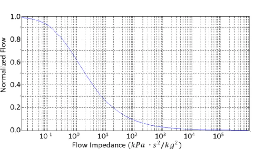
simulation to represent different fouling conditions. The plot of the flow vs the flow impedance is shown in Fig. 2.4. A change inzc affects m˙c and thus affects the heat transfer and the output

temperatures of hot and cold air streams as computed using Eq. (2.1)-(2.3). This also affects the sensor readings of all other sensors in the ECS.

2.3.2 Data Generation Process

This chapter utilizes an experimentally validated high-fidelity Simulink model of the ECS provided by an industry partner. The model is used to generate dynamic data for various sensor locations around the ECS system for fouling diagnosis. It is important to note that the model represents the ECS performance for a specific aircraft and has been validated to match experimental results from lab testing and flight data for this specific ECS. For this chapter, the model is exercised to generate time series of sensor data for various ground operating conditions (e.g., ambient temperature, oc-cupant count, etc.). Ground operating conditions are chosen because typically more debris exists in the aircraft vicinity while on the ground as opposed to in-flight operation. Data generated for this study includes a large number (>100) of sensor outputs.

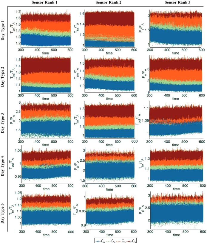
Figure 2.5 shows the stochastic time series data plots of three critical sensors under various uncertainties for different day types. The structure of the data is explained below. Let us denote the sensor suite by a set

S

generating a data sequencez_j = [z_j(1), ...z_j(600)], ∀j = 1,2, . . . m. The system reaches steady state after 300 seconds, thus the data from301to600 seconds is used for analysis; however this interval could be reduced for higher sampling rates.

It is to be noted that the system behavior and the sensor data are affected by several input parameters, which affect the accuracy of fouling diagnosis. This chapter considers variations in two main input parameters: the ambient temperature for different day types and the load corresponding to different occupant counts on the aircraft. Besides the heat exchanger fouling itself results in variations in sensor data. Thus the objective is to capture the effects of fouling under different input conditions. Specifically, the data is generated by varying the aforementioned parameters as described below.

•Ambient Temperature (TA)

As expected, the ambient temperature is the most critical external parameter that affects sensor readings. The effect of ambient temperature could be misinterpreted and could lead to false di-agnosis of heat exchanger fouling. Thus, to incorporate the effect of ambient temperature, sensor data is categorized into five different day types: i) extremely cold, ii) cold, iii) medium, iv) hot and v) extremely hot day types. The temperature ranges for each day type are shown in Table 2.2(a). Each day type is further partitioned into eight uniformly spaced temperature values.

•Occupant Count (OCC)

The occupant count also affects ECS sensor readings due to passengers adding heat load that the ECS reacts to in order to maintain the desired cabin conditions. The number of occupants is grouped into four categories: i) Low Load, ii) Medium Load, iii) Heavy Load, and iv) Very Heavy Load based on the percentage occupancy in the cabin. Table 2.2(b) shows these four load categories. Since OCC has relatively less influence on the sensor readings, only the middle point of each category is used for data generation.

C

0 C1 C2 C3

Sensor Rank 1 Sensor Rank 2 Sensor Rank 3

D a y T y p e 1 D a y T y p e 2 D a y T y p e 3 D a y T y p e 4 D a y T y p e 5

Table 2.2: Input Parameters and Fouling Classes (a) Day Types

Day Type Tamb(oF)

Extremely cold -30 – 0 Cold 0 – 30 Medium 30 – 60 Hot 60 – 90 Extremely hot 90 – 120

(b) Passenger Load Categories

Load Type OCC

Low Load 0% – 60% Medium Load 60% – 75% Heavy Load 75% – 95% Very Heavy Load 95% – 100%

(c) Fouling Classes Class Flow Green (c0) 80% – 100% Yellow (c1) 60% – 80% Orange (c2) 40% – 60% Red (c3) 0% – 40%

•Heat Exchanger Fouling (zc)

Fouling of the secondary heat exchanger is modeled as an increase in the ram air-flow impedance (zc) on the cold side of the heat exchanger. When the flow impedance is increased, the air-flow

decreases simulating blockage due to heat exchanger fouling. This lowers the effectiveness of the heat exchanger. For this chapter, four fouling classes have been defined based on the flow through the cold-side of the secondary heat exchanger as follows: i)Green Class(c0)- i.e., 80-100

%flow, ii)Yellow Class(c1)- i.e., 60-80%flow, iii)Orange Class(c2)- i.e., 40-60%flow, and iv)

Red Class(c3)- i.e., 0-40%flow. The reason to introduce Yellow and Orange classes is to avoid

direct confusion between the Green and Red classes. The model is run for different values of flow impedance and the resulting flow through the heat exchanger is observed. The plot in Fig. 2.4 is used to determine the range of impedance values for each of the above classes that are defined based on the flow. Table 2.2(c) shows the impedance intervals associated with each class. Each class is further partitioned into eight uniformly spaced flow values for data generation.

Thus, for each day type stochastic time series data are generated for various combinations of the above parameters to represent each fouling class. The model is run for different combinations of the values of ambient temperature (8) (within each day type), occupant counts (4), and impedance values (8) (within each fouling class), resulting in a set consisting of a total number of8×4×8=

256runs of time series data. Furthermore, for each day type, similar data sets are generated for all the fouling classes, thus leading to a total of4×256=1024runs of time series data. Subsequently, the above data sets are generated for all five day types. Let Γ = {γ1, ...γ1024} denote the set of

parametric combinations and let t ∈ {1,2, ...T} denote the set of discrete time indices, where T = 600is the length of the time series data. Then, for each day type the entire data for each

sensors_j ∈

S

2.3.3 Heat Exchanger Fouling Diagnosis Architecture

Figure 2.3 shows the Heat exchanger fouling diagnosis architecture that consists of a training and a testing phase. The training phase consists of generating stochastic data for each sensor in the ECS (total 109 sensors) as described above. This sensor data is labeled with the fouling class information and is used for optimal sensor selection for each day type separately, as described in Section 2.4. From the data of optimal sensors, some useful features are extracted using PCA and GMM methods and classifiers (k-NN) are trained to identify the fouling classes, as described in Section 2.5.

In the testing phase, an unlabeled time series data is generated for an unknown parametric con-ditionγ ∈Γwhere the fouling severity is also considered as unknown. Subsequently, the optimal sensors identified in training phase are used for feature extraction and classification using trained classifiers. To further improve the classification accuracy, the results of the top three optimal sen-sors are fused using the majority vote.

2.4

Optimal Sensor Selection Methodology

Since a large number of sensors are available in the ECS mounted at different locations, the underlying processes of data generation, storage, and analysis become cumbersome. Therefore, an optimal sensor selection methodology is needed to rank the most relevant sensors in terms of the

best classification performance for heat exchanger fouling diagnosis. This is formally stated in the following problem statement.

Optimal Sensor Selection Problem: Given the sensor set

S

sen-sors, and the class set

C

is to select a set

S

S

S

classification accuracy and are ranked accordingly in decreasing order.

As discussed in the introduction, two commonly used sensor selection methods are: i) the

wrapper method and ii) the filter method. Since the wrapper algorithms rank the sensors based

on their correct classification rate (CCR), a feature extractor and a classifier have to be designed, trained, and applied to all sensors in order to compute their CCRs, thus making the whole process computationally expensive. Furthermore, the wrapper algorithms cannot be generalized to any classifier [12–14]. On the other hand, the filter algorithms evaluate the performance of each sensor based on an information theoretic measure [10, 15]. Filter algorithms are computationally less expensive and do not depend on the choice of a classifier, but they may not perform as good as the wrapper algorithms [13].

To circumvent this difficulty, the embedded algorithms take advantage of both the wrapper and the filter algorithms by using a filter to select a candidate list of sensors and then applying a wrapper on this list to rank and select the optimal set of sensors [10]. Embedded algorithms are less expensive than wrappers and more accurate than filters; yet they are pertinent to the specified classifier [16]. In this regard, this section presents a detailed description of the optimal sensor set selection methodology based on theembedded algorithm. In addition, a novel algorithm for sensor selection is presented, called the unsupervised embedded algorithm, that relies on the K-means clustering approach. This method has the advantage that it does not depend on the choice of a classifier and enables faster execution with very low computational complexity.

Both the embedded and the unsupervised embedded algorithms are based on the minimum

Re-dundancy Maximum Relevance (mRMR) [10] criteria for the filter algorithm as a precursor step

re-duction and produces a candidate list of top ranked sensors. Before describing the optimal sensor selection techniques, some useful information-theoretic quantities are defined below.

2.4.1 Information-theoretic Measures

Definition 2.4.1 (Entropy) Entropy H(X) is defined as a measure of uncertainty in a random

variableX such that

H(X) =−

|X|

X

i=1

pilnpi (2.5)

whereX is a random variable whose outcomes belong to the set

X

associated probability distribution defined asp(X =xi) = pi ∀i= 1,2, . . .|

X

According to Shannon [62], the entropyH(X)qualifies to be a measure of uncertainty because it satisfies the following three conditions:

• H(X)is a continuous function ofpi.

• If the random variable X is uniformly distributed (i.e., pi = _|X1_|, ∀i = 1,2, . . .|

X

H(X)is a monotonically increasing function of|

X

• If an event X = xi is split into two posterior sub-events, then the original entropy can be

expressed as a weighted sum of the entropies of the sub-events.

The higher the entropy is, the higher is the uncertainty in the random variable. On the other hand, the entropy reaches its lowest value,H(X) = 0, whenp(X)is a delta distribution.

Suppose now that we have two random variables: X defined as above, andY whose outcomes belong to the set

Y

Y

Furthermore, suppose that the joint probability distribution is defined aspi,j =p(X =xi, Y =yj)

follows: H(X, Y) =− |X| X i=1 |Y| X j=1 p_i,jlnp_i,j (2.6) H(X|Y) =− |X| X i=1 |Y| X j=1 p_i,jlnp(X =x_i|Y =y_j) =H(X, Y)−H(Y) (2.7)

Definition 2.4.2 (Mutual Information) The mutual information between two random variables

XandY is defined as

I(X, Y) =H(X)−H(X|Y)

=H(X) +H(Y)−H(X, Y) (2.8)

The subtraction ofH(X|Y)fromH(X)represents the information gained about the random vari-ableX given the information about the random variableY [15]. The next section presents a parti-tioning approach for transformation of the continuous data to the symbolic domain for computation of the information-theoretic quantities as needed in the filter method.

2.4.2 Data Partitioning for Symbol Sequence Generation

Consider the data matrixZj of size|Γ| ×T for any particular sensorsj, j = 1,2, ...m, generated

under different parametric conditions as described in Section 2.3.2. The encoding of the underlying dynamics of this sensor data is achieved by partitioning [63] of the sensor observation space using an appropriate partitioning method. LetRj ⊂

R

within which the observed sensor data Zj is circumscribed. Let Σ = {α1, α2, . . . α|Σ|} be the

symbol alphabet that labels the partition segments, where the number of segments is |Σ|, where

2 ≤ |Σ| < ∞. Then, the symbolic encoding of Rj is accomplished by introducing a partition {ϕ1_j,· · · , ϕ|_jΣ|}consisting of|Σ|mutually exclusive (i.e.,ϕ`<sub>j</sub> ∩ϕk<sub>j</sub> = ∅, ∀` 6= k), and exhaustive (i.e., S|Σ|

r=1ϕrj = Rj) cells. Each cell is encoded with a symbol from the alphabet Σ. For each

different cells of the partition, accordingly the corresponding symbol is assigned to each point of the trajectory. Let z_j(γ_r) _, [Z_j(r,1), Z_j(r,2), . . . Z_j(r, T)] be the rth row of the data matrix Z_j for a givenγr ∈Γ. Then, for each sensorsj ∈

S

are transformed into a symbol sequence [64]˜zj(γr),[ ˜Zj(r,1), . . .Z˜j(r, T)]as

[Zj(r,1), . . . Zj(r, T)]→[ ˜Zj(r,1), . . .Z˜j(r, T)] (2.9)

whereT is the data length, Z˜j(r, t) ∈ Σ, ∀t = 1, ...T and Z˜j is the symbolic data matrix. Note:

As mentioned earlier, this chapter uses only the steady state part of the data for fouling diagnosis analysis (i.e.,∀t= 301,302, . . .600).

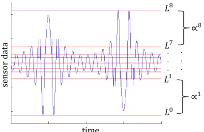
To do the above symbolization, this chapter uses the maximum entropy principle [65] based partitioning to create a partition of the observed sensor data space, which is finer in the information dense regions and coarser in the low information regions as described below.

Definition 2.4.3 (Maximum Entropy Principle, Jaynes [65]) The maximum entropy principle states

that the probability distribution that unbiasedly estimates the distribution of a random variableX

under a given set of constraints is the distribution that maximizes the entropyH(X).

In other words, the unbiased estimate of the probability distribution of a random variableXshould satisfy the following optimization problem:

P∗ =       p∗₁ .. . p∗ |X|       = arg max P H(X); H(X) = − |X| X i=1 pilnpi subject to: |X| X i=1 pi = 1 (2.10)

The optimization problem in Eq. (2.10) can be solved using the Lagrange multiplier as shown in Appendix A.1. As a result, the entropy is maximized for the uniform distribution (i.e., p∗_i =

1

|X|, ∀i= 1, ...|

X

readings. Considering the data matrix Z_j = [Z_j(r,1), Z_j(r,2), . . . Z_j(r, T)]_r=1,...|Γ|for sensor s_j, the goal is to find the partition that results in maximum entropy distribution (i.e., the uniform distribution). The partition cells are defined by the partitioning levels

L

floor(|Γ| × T /|Σ|), ∀r = 1,2, ...|Σ|). The second step is to sort the entire data into a vector

wj = [wj(1), wj(2), . . . wj(|Γ| ×T)], such that

wj(`)∈ {Zj(r, t)∀r= 1,2. . .|Γ|, t= 1,2, . . . T} ∀` = 1,2, . . .|Γ| ×T (2.11)

& wj(1)≤wj(2). . .≤wj(|Γ| ×T) (2.12)

Then the partitioning levels are defined as follows:

L0_j =wj(1) (2.13)

Lq_j =wj(q·η∗)∀q= 1, . . .|Σ| −1, and (2.14)

L|_jΣ|=w_j(|Γ| ×T) (2.15)

The algorithm counts the samples from the bottom and defines the partitioning levels at the multi-ples ofη∗while setting the first and the last levels at the min and the max of the original data. This procedure generates a partition that is finer in the regions of high data density and coarser in the regions of low data density, as shown by an illustrative example in Fig. 2.6. Subsequently, a unique symbol from the alphabetΣis assigned to all the data points in each cell of the partitioning. This process transforms each data matrix inZj into a symbol matrixZ˜j, as shown in Eq. (2.9).

In the above manner, the maximum entropy partitioning is constructed for all sensors and the corresponding data are transformed into symbol sequences. Subsequently, the candidate list of sensors is selected and ranked according to the filter criteria as described next.

2.4.3 minimum Redundancy Maximum Relevance (mRMR)

Based on mutual information, the mRMR criterion [10] evaluates and ranks the sensors that best describe the classes and simultaneously avoid sensors that provide redundant information by means

Figure 2.6: An illustration of the Maximum Entropy Partitioning

of the following two conditions: i) Maximum Relevance and ii) Minimum Redundancy, as de-scribed below.

Let us define the random variablesCandSj,j = 1, ...m, as follows:

• C: A random variable whose sample space is the set of all symbol sequences and its outcome belongs to the class set

C

• Sj: A random variable whose sample space is the symbolized data matrix˜zj for sensorsjand

its outcome belongs toΣ.

Then the Maximum Relevance criteria is defined as follows.

Definition 2.4.4 (Max Relevance) The Maximum Relevance criterion aims to find the set

U

S

U

1| = m∗, m∗ < m, that has the maximum average mutual information between its

sensors and the random variableC, such that

U

U

U

The Maximum-Relevance criterion does not account for the information redundancy between sensors. Thus, the Minimum Redundancy criteria is defined as follows.

S

U

2| = m∗, m∗ < m, that minimizes average mutual information between its sensor

pairs, such that

U

U

U

The mRMR criterion combines the above two criterion as follows.

Definition 2.4.6 (minimum Redundancy Maximum Relevance) The minimum Redundancy

Max-imum Relevance (mRMR) criterion aims to find the set

S

S

S

optimizeJ1 andJ2simultaneously, such that

S

U⊆S,|U|=m∗J(

U, C

J(

U, C

U, C

U

The evaluation of the mRMR criteria requires: a) computation of I(Sj, C) and I(S`, Sj), ∀`, j = 1,2, . . . m, and b) finding the solution of the optimization function in Eq. (2.18). The mutual information quantities are computed from the symbol sequences of each sensor data, as described in Appendix A.2. The optimization problem based on the mRMR criterion is a com-binatorial problem, which can be solved using theForward Selection search method [10]. Note: this information-theoretic method of sensor selection is more efficient and several orders of mag-nitude faster as compared to the full wrapper method that requires computation of the CCRs for all sensors.

Forward Selection Search

The forward selection search is a greedy search algorithm that is used to find a (sub)optimal solu-tion of the mRMR optimizasolu-tion problem in Eq. (2.18). To be specific, the algorithm starts with an empty set of sensors, then keep adding sensors that maximize the mRMR criteria until the desired number ofmsensors is obtained. The details [66] of the algorithm are shown in Algorithm 1.

Result:An optimal set of sensorsS∗={s∗<sub>`</sub>, ∀`= 1,2, . . . m∗}.

Initialization:S={s1, s2, . . . sm},S∗=∅,`= 1

while`≤m∗do

• Step 1: Find the sensors∗_` ∈Sthat maximizes the criterion in Eq. (2.18) for a single sensor

• Step 2: UpdateS→S−s∗_`

• Step 3: UpdateS∗_→S∗_∪s∗

`, `→`+ 1

end

Algorithm 1:The Forward Selection Search Algorithm

2.4.4 Embedded Algorithm

As mentioned earlier, anembedded wrapper and filteralgorithm is used to tradeoff between the low complexity of filter algorithms and the accuracy of wrapper algorithms in the optimal sensor set selection procedure. In other words, an embedded algorithm uses a filter algorithm first to select a

candidate list(CL) of sensors; subsequently, a wrapper algorithm (which uses a specific classifier)

is deployed to select or rank theoptimal set of sensors[10] from the candidate list. The embedded algorithms also have several deficiencies including being classifier specific and requiring tuning the classifier beforehand for each sensor separately. To circumvent these disadvantages, the paper proposes the unsupervised embedded algorithm as described next.

2.4.5 Unsupervised Embedded Algorithm

The unsupervised embedded algorithm also relies on a filter algorithm (e.g., the mRMR) to select the candidate list (CL) of m sensors. Then the data Zj corresponding to each sensor sj ∈ CL,

which consists of the data of all classes, are clustered intonclusters using theK-means clustering algorithm [67], where n is equal to the number of fouling classes (for this paper n = 4). Lets call these clusters as{

O

O

O

cluster

O

C

entropy H(Oi), i = 1, . . . n, of the class distribution within each cluster is computed using Eq.

(2.5). Then, the weighted entropy sensorsj is calculated as

H_j = n X i=1 |

O

ŶĞdžĂŵƉůĞŽĨĂďĂĚƐĞŶƐŽƌ_ݏ݆ ŶƚƌŽƉLJܪ݆_ŝƐŚŝŐŚ ܱ௠௜ ĂŶĚܱ௠௝ ĂƌĞƚŚĞĐůƵƐƚĞƌƐƌĞƐƵůƚĞĚĨƌŽŵ<Ͳ ŵĞĂŶƐĨŽƌŐŽŽĚĂŶĚďĂĚƐĞŶƐŽƌƐ׊ ݅ǡ ݆с ϭ͕Ϯ͕͙ϭϬ͕ŵсϭ͕Ϯ͕ϯ͕ϰ

ܱ

ܱ

ܱ

ܱ

Đ

Đ

Đ

Đ

ܱ

ܱ

ܱ

ܱ

džĂŵƉůĞŽĨ

<

ͲŵĞĂŶƐŝŶZ

^ƉĂĐĞ

Đ

Đ

Đ

Đ

(a) High-ranking, low-entropy sensor

ŶĞdžĂŵƉůĞŽĨĂďĂĚƐĞŶƐŽƌݏ݆ ŶƚƌŽƉLJܪ݆_ŝƐŚŝŐŚ ܱ௠௜ ĂŶĚܱ௠௝ ĂƌĞƚŚĞĐůƵƐƚĞƌƐƌĞƐƵůƚĞĚĨƌŽŵ<Ͳ ŵĞĂŶƐĨŽƌŐŽŽĚĂŶĚďĂĚƐĞŶƐŽƌƐ׊ ݅ǡ ݆с ϭ͕Ϯ͕͙ϭϬ͕ŵсϭ͕Ϯ͕ϯ͕ϰ

ܱ

ܱ

ܱ

ܱ

ܱ

ܱ

ܱ

ܱ

džĂŵƉůĞŽĨ

<

ͲŵĞĂŶƐŝŶZ

^ƉĂĐĞ

(b) Low-ranking, high-entropy sensor

Oi: a cluster∀i= 1,2,3,4 ci: classes∀i= 0,1,2,3

Figure 2.7: An example of using the K-means clustering algorithm and the entropy criterion to rank sensors

where|Γ| ·T =

n

P

i=1

|

O

Finally, the sensors are ranked according to their entropies such that the sensor that has the lowest entropy is ranked the highest and so on. In this fashion the candidate list is re-ranked and a possible list of top ranked sensors is selected for further analysis. This process ranks the sensors in the order such that the sensors that have the least uncertainty between classes in their data clusters are ranked the highest, thus facilitating a better classification decision.

Figures 2.7(a) and 2.7(b) show examples of a high and low rank sensors, respectively. As seen in the figures, when the average entropyH_j for a sensor s_j ∈

S

between samples that belong to different classes are high while the within-class distances (i.e., distances between samples that belong to the same class) are low. Therefor, low entropy sensors are expected to achieve higher CCRs.

2.5

Data Analysis for Fouling Diagnosis

Once an optimal sensor set is obtained, different machine learning methods are applied for analysis of sensor data for fouling diagnosis. These methods consists of the feature extraction and the classification steps as described below.

2.5.1 Feature Extraction

Two methods of feature extraction are applied in this chapter; namely, the Principal Component

Analysis(PCA) and theGaussian Mixture Model(GMM) as described below.

Principal Component Analysis (PCA)

The Principal Component Analysis (PCA) is a data reduction method. Given a data matrix X

of dimension L ×m, where L > m, whose columns are data vectors (e.g., sensor data). The objective of PCA is to transform the data matrixX into a matrixX0 of sizeL×m0, where m0 < m. The columns of X0 hold theScore Vectors (also known as the Principal Components). This transformation is accomplished using the Karhunen-Lo´eve(KL) algorithm which is summarized in Appendix B.1. For implementation to the heat exchanger data, consider the sensor dataZj for a

specific sensorsj for a specific day type. The nominal data corresponding to classc0 is extracted

fromZj and averaged to get a time series data¯z0j as follows:

¯z0_j = 1 256

X

γ∈{γ1...γ256}

z0_j(γ) (2.20)

Thereafter, the steady state part of¯z0_j is partitioned intom = 10segments, each of lengthL= 30. These data segments are organized to form a L × m data matrix X0. Following the steps of the KL algorithm, the m × m0 transformation matrix Ω is then obtained, where m0 = 2 and is kept fixed. Subsequently, the scores (or principal components) of any observation sequence zj(γ) ∀γ = 1,2, . . .|Γ| are generated by reorganizing the sequence into anL×m matrixX by

breakingz_j(γ)intom segments of lengthLeach. The scores of this sequence are then computed using Eq. (B.1) in Appendix B.1. These scores consist of L points each of which are m0 = 2

dimensional. In the training phase these scores are labeled with fouling class and are sent to the classifier for training, while in the testing phase they are unlabeled and are sent to the trained classifier for decision on the fouling class.

Gaussian Mixture Model (GMM)

Consider sensor data z_j(γ_r) = [Z_j(r,1), Z_j(r,2), . . . Z_j(r, T)] for some γ_r ∈ Γ. The Gaussian Mixture Model (GMM) is a statistical model ofz_j(γ_r)represented as a sum ofRdifferent Gaussian distributions as p(zj(γr)|

M

G

whereM = {ρ1, ρ2, . . . ρR, µ1, µ2, . . . µR, σ1, σ2, . . . σR}is the set of weightsρ`s, meansµ`s and variances σ`s, ` = 1, . . . R, and z is a random variable. The function

G

G

The parametersρ`, µ` andρ`,∀` = 1,2, . . . R, are estimated from the data using theExpectation

Maximization(EM) algorithm [68]. Subsequently,

M

implementation to the heat exchanger data, a GMM is constructed from sensor data withR = 2. For each observation sequencezj(γr)∀r = 1,2, . . .|Γ|inZj, the feature set

M

as

M

2.5.2 Classification

Once the features are obtained as the principal components or the parameter set of the GMM, they are processed by a classifier to make a decision on the heat exchanger fouling severity. This section describes thek-Nearest Neighbor (k-NN) algorithm that is used as the classification technique.

k-Nearest Neighbor (k-NN)

The k-Nearest Neighbor (k-NN) classification algorithm is popular for its simplicity, efficiency and low complexity. The k-NN classifier is explained in Appendix B.3. For implementation,

thek-NN classifier is applied on the feature space generated by PCA and GMM for each sensor in the candidate list and each day type. For each observation sequence z_j(γ_r), the PCA based features (i.e., principal components) are L = 30 dimensional vectors in m0 = 2 dimensional feature space while the GMM based features (i.e. the pa