Representing Meaning with a Combination of Logical and Distributional Models

of Logical and Distributional Models

I. Beltagy

The University of Texas at Austin

Stephen Roller

The University of Texas at Austin

Pengxiang Cheng

The University of Texas at Austin

Katrin Erk

The University of Texas at Austin

Raymond J. Mooney

The University of Texas at Austin

NLP tasks differ in the semantic information they require, and at this time no single seman-tic representation fulfills all requirements. Logic-based representations characterize sentence structure, but do not capture the graded aspect of meaning. Distributional models give graded similarity ratings for words and phrases, but do not capture sentence structure in the same detail as logic-based approaches. It has therefore been argued that the two are complementary.

We adopt a hybrid approach that combines logical and distributional semantics using probabilistic logic, specifically Markov Logic Networks. In this article, we focus on the three components of a practical system:11)Logical representationfocuses on representing the input problems in probabilistic logic; 2)knowledge base construction creates weighted inference rules by integrating distributional information with other sources; and 3)probabilistic in-ference involves solving the resulting MLN inference problems efficiently. To evaluate our approach, we use the task of textual entailment, which can utilize the strengths of both logic-based and distributional representations. In particular we focus on the SICK data set, where we achieve state-of-the-art results. We also release a lexical entailment data set of 10,213 rules extracted from the SICK data set, which is a valuable resource for evaluating lexical entailment systems.2

∗Computer Science Department, The University of Texas at Austin. E-mail:{beltagy, roller, pxcheng}@cs.utexas.edu.

∗∗Linguistics Department, The University of Texas at Austin. E-mail:[email protected]. 1 System is available for download at:https://github.com/ibeltagy/pl-semantics.

2 Available at:https://github.com/ibeltagy/rrr.

1. Introduction

Computational semantics studies mechanisms for encoding the meaning of natural language in a machine-friendly representation that supports automated reasoning and that, ideally, can be automatically acquired from large text corpora. Effective semantic representations and reasoning tools give computers the power to perform complex applications like question answering. But applications of computational semantics are very diverse and pose differing requirements on the underlying representational for-malism. Some applications benefit from a detailed representation of the structure of complex sentences. Some applications require the ability to recognize near-paraphrases or degrees of similarity between sentences. Some applications require inference, either exact or approximate. Often, it is necessary to handle ambiguity and vagueness in meaning. Finally, we frequently want to learn knowledge relevant to these applications automatically from corpus data.

There is no single representation for natural language meaning at this time that fulfills all of these requirements, but there are representations that fulfill some of them. Logic-based representations (Montague 1970; Dowty, Wall, and Peters 1981; Kamp and Reyle 1993), like first-order logic, represent many linguistic phenomena like negation, quantifiers, or discourse entities. Some of these phenomena (especially negation scope and discourse entities over paragraphs) cannot be easily represented in syntax-based representations like Natural Logic (MacCartney and Manning 2009). In addition, first-order logic has standardized inference mechanisms. Consequently, logical approaches have been widely used in semantic parsing where it supports answering complex natural language queries requiring reasoning and data aggregation (Zelle and Mooney 1996; Kwiatkowski et al. 2013; Pasupat and Liang 2015). But logic-based representations often rely on manually constructed dictionaries for lexical semantics, which can result in coverage problems. And first-order logic, being binary in nature, does not capture the graded aspect of meaning (although there are combinations of logic and proba-bilities). Distributional models (Turney and Pantel 2010) use contextual similarity to predict the graded semantic similarity of words and phrases (Landauer and Dumais 1997; Mitchell and Lapata 2010), and to model polysemy (Sch ¨utze 1998; Erk and Pad ´o 2008; Thater, F ¨urstenau, and Pinkal 2010). But at this point, fully representing structure and logical form using distributional models of phrases and sentences is still an open problem. Also, current distributional representations do not support logical inference that captures the semantics of negation, logical connectives, and quantifiers. Therefore, distributional models and logical representations of natural language meaning are com-plementary in their strengths, as has frequently been remarked (Coecke, Sadrzadeh, and Clark 2011; Garrette, Erk, and Mooney 2011; Grefenstette and Sadrzadeh 2011; Baroni, Bernardi, and Zamparelli 2014).

For logic-based semantics, one of the challenges is to adapt the representation to the assumptions of the probabilistic logic (Beltagy and Erk 2015). For distributional lexical and phrasal semantics, one challenge is to obtain appropriate weights for inference rules (Roller, Erk, and Boleda 2014). In probabilistic inference, the core challenge is formulating the problems to allow for efficient Markov Logic Network (MLN) inference (Beltagy and Mooney 2014).

Our approach has previously been described in Garrette, Erk, and Mooney (2011) and Beltagy et al. (2013). We have demonstrated the generality of the system by applying it to both textual entailment (RTE-1 in Beltagy et al. [2013], SICK [preliminary results] and FraCas in Beltagy and Erk [2015]) and semantic textual similarity (Beltagy, Erk, and Mooney 2014), and we are investigating applications to question answering. We have demonstrated the modularity of the system by testing both MLNs (Richardson and Domingos 2006) and Probabilistic Soft Logic (Broecheler, Mihalkova, and Getoor 2010) as probabilistic inference engines (Beltagy et al. 2013; Beltagy, Erk, and Mooney 2014).

The primary aim of the current article is to describe our complete system in detail— all the nuts and bolts necessary to bring together the three distinct components of our approach—and to showcase some of the difficult problems that we face in all three areas, along with our current solutions.

The secondary aim of this article is to show that it is possible to take this general approach and apply it to a specific task—here, textual entailment (Dagan et al. 2013)— adding task-specific aspects to the general framework in such a way that the model achieves state-of-the-art performance. We chose the task of textual entailment because it utilizes the strengths of both logical and distributional representations. We specifically use the SICK dataset (Marelli et al. 2014b) because it was designed to focus on lexical knowledge rather than world knowledge, matching the focus of our system.

Our system is flexible with respect to the sources of lexical and phrasal knowledge it uses, and in this article we utilize PPDB (Ganitkevitch, Van Durme, and Callison-Burch 2013) and WordNet, along with distributional models. But we are specifically interested in distributional models, in particular, in how well they can predict lexical and phrasal entailment. Our system provides a unique framework for evaluating distributional models on recognizing textual entailment (RTE) because the overall sentence represen-tation is handled by the logic, so we can zoom in on the performance of distributional models at predicting lexical (Geffet and Dagan 2005) and phrasal entailment. The eval-uation of distributional models on RTE is the third aim of our article. We build a lexical entailment classifier that exploits both task-specific features as well as distributional information, and present an in-depth evaluation of the distributional components.

We now provide a brief sketch of our framework (Garrette, Erk, and Mooney 2011; Beltagy et al. 2013). Our framework is three components. The first is the logical form, which is the primary meaning representation for a sentence. The second is the distri-butional information, which is encoded in the form ofweightedlogical rules (first-order formulas). For example, in its simplest form, our approach can use the distributional similarity of the wordsgrumpyandsadas the weight on a rule that says ifxis grumpy, then there is a chance thatxis also sad:

∀x.grumpy(x)→sad(x)|f(sim(grumpy~ ,sad~ ))

similarity score to an MLN weight. A more principled, and in fact, superior, choice is to use an asymmetric similarity measure to compute the weight, as we discuss subsequently.

The third component is inference. We draw inferences over the weighted rules using MLNs (Richardson and Domingos 2006), a Statistical Relational Learning tech-nique (Getoor and Taskar 2007) that combines logical and statistical knowledge in one uniform framework, and provides a mechanism for coherent probabilistic infer-ence. MLNs represent uncertainty in terms of weights on the logical rules, as in this example:

∀x.ogre(x)⇒grumpy(x)|1.5

∀x,y.(friend(x,y)∧ogre(x))⇒ogre(y)|1.1 (1)

which states that there is a chance that ogres are grumpy, and friends of ogres tend to be ogres too. Markov logic uses such weighted rules to derive a prob-ability distribution over possible worlds through an undirected graphical model. This probability distribution over possible worlds is then used to draw infer-ences.

We publish a data set of the lexical and phrasal rules that our system queries when running on SICK, along with gold standard annotations. The training and testing sets are extracted from the SICK training and testing sets, respectively. The total number of rules (training + testing) is 12,510—only 10,211 are unique with 3,106 entailing rules, 177 contradictions, and 6,928 neutral. This is a valuable resource for testing lexical en-tailment systems, containing a variety of enen-tailment relations (hypernymy, synonymy, antonymy, etc.) that are actually useful in an end-to-end RTE system.

In addition to providing further details on the approach introduced in Garrette, Erk, and Mooney (2011) and Beltagy et al. (2013) (including improvements that improve the scalability of MLN inference [Beltagy and Mooney 2014] and adapt logical constructs for probabilistic inference [Beltagy and Erk 2015]), this article makes the following new contributions:

r

probabilistic logic (Sections 4.1, 4.2), arguing for the use of a closed-word assumption (Section 4.3).

r

assumption about entity coreference. For example,An ogre is not snoring andAn ogre is snoringare not contradictory unless we assume that the two ogres are the same. Handling such coreferences is important to detecting many cases of contradiction (Section 4.4).

r

r

in particular WordNet (Princeton University 2010) and the paraphrase collection PPDB (Ganitkevitch, Van Durme, and Callison-Burch 2013) (Section 5.3).

r

r

the SICK data set (10,211 rules). This is a valuable resource for testing lexical entailment systems on entailment relations that are actually useful in an end-to-end RTE system

(Section 5.1).

r

(Paperno, Pham, and Baroni 2014) on the task of phrasal entailment (Section 5.2.5).

r

MLN weights (Section 6.3).

r

inference relations?” (Levy et al. 2015) has been studied before on a variety of lexical entailment data sets. For the first time, we study it on data from an actual RTE data set and show that distributional information is useful for lexical entailment (Section 7.1).

r

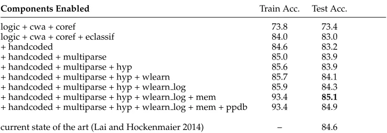
2014, the best result was achieved by systems that did not compute a sentence representation in a compositional manner. We present a model that performs deep compositional semantic analysis and achieves state-of-the-art performance (Section 7.2).

2. Background

Logical Semantics.Logical representations of meaning have a long tradition in lin-guistic semantics (Montague 1970; Dowty, Wall, and Peters 1981; Alshawi 1992; Kamp and Reyle 1993) and computational semantics (Blackburn and Bos 2005; van Eijck and Unger 2010), and are commonly used in semantic parsing (Zelle and Mooney 1996; Berant et al. 2013; Kwiatkowski et al. 2013). They handle many complex semantic phenomena, such as negation and quantifiers, and they identify discourse referents along with the predicates that apply to them and the relations that hold between them. However, standard first-order logic and theorem provers are binary in nature, which prevents them from capturing the graded aspects of meaning in language: Synonymy seems to come in degrees (Edmonds and Hirst 2000), as does the difference between senses in polysemous words (Brown 2008). van Eijck and Lappin (2012) write: “The case for abandoning the categorical view of competence and adopting a probabilistic model is at least as strong in semantics as it is in syntax.”

Recent wide-coverage tools that use logic-based sentence representations include Copestake and Flickinger (2000), Bos (2008), and Lewis and Steedman (2013). We use Boxer (Bos 2008), a wide-coverage semantic analysis tool that produces logical forms, using Discourse Representation Structures (Kamp and Reyle 1993). It builds on the C&C CCG (Combinatory Categorial Grammar) parser (Clark and Curran 2004) and maps sentences into a lexically based logical form, in which the predicates are mostly words in the sentence. For example, the sentenceAn ogre loves a princessis mapped to:

As can be seen, Boxer uses a neo-Davidsonian framework (Parsons 1990):yis an event variable, and the semantic rolesagentandpatientare turned into predicates linkingyto the agentxand patientz.

As we discuss later, we combine Boxer’s logical form with weighted rules and perform probabilistic inference. Lewis and Steedman (2013) also integrate logical and distributional approaches, but use distributional information to create predicates for a standard binary logic and do not use probabilistic inference. Much earlier, Hobbs et al. (1988) combined logical form with weights in an abductive framework. There, the aim was to model the interpretation of a passage as its best possible explanation.

Distributional Semantics.Distributional models (Turney and Pantel 2010) use statis-tics on contextual data from large corpora to predict semantic similarity of words and phrases (Landauer and Dumais 1997; Mitchell and Lapata 2010). They are motivated by the observation that semantically similar words occur in similar contexts, so words can be represented as vectors in high dimensional spaces generated from the contexts in which they occur (Lund and Burgess 1996; Landauer and Dumais 1997). Therefore, distributional models are relatively easier to build than logical representations, auto-matically acquire knowledge from “big data,” and capture thegradednature of linguistic meaning, but they do not adequately capture logical structure (Grefenstette 2013).

Distributional models have also been extended to compute vector representa-tions for larger phrases, for example, by adding the vectors for the individual words (Landauer and Dumais 1997) or by a component-wise product of word vectors (Mitchell and Lapata 2008, 2010), or through more complex methods that compute phrase vec-tors from word vecvec-tors and tensors (Baroni and Zamparelli 2010; Grefenstette and Sadrzadeh 2011).

Integrating Logic-Based and Distributional Semantics.It does not seem particularly use-ful at this point to speculate about phenomena that either a distributional approach or a logic-based approach would not be able to handle in principle, as both frameworks are continually evolving. However, logical and distributional approaches clearly differ in the strengths that they currently possess (Coecke, Sadrzadeh, and Clark 2011; Garrette, Erk, and Mooney 2011; Baroni, Bernardi, and Zamparelli 2014). Logical form excels at in-depth representations of sentence structure and provides an explicit representation of discourse referents. Distributional approaches are particularly good at representing the meaning of words and short phrases in a way that allows for modeling degrees of similarity and entailment and for modeling word meaning in context. This suggests that it may be useful to combine the two frameworks.

Another argument for combining both representations is that it makes sense from a theoretical point of view to address meaning, a complex and multifaceted phe-nomenon, through a combination of representations. Meaning is about truth, and logical approaches with a model-theoretic semantics nicely address this facet of meaning. Meaning is also about a community of speakers and how they use language, and distributional models aggregate observed uses from many speakers.

There are few hybrid systems that integrate logical and distributional information, and we discuss some of them here.

forms. The main difference between the two approaches lies in the role of gradience. Lewis and Steedman view weights and probabilities as a problem to be avoided. We believe that the uncertainty inherent in both language processing and world knowl-edge should be front and center in all inferential processes. Tian, Miyao, and Takuya (2014) represent sentences using Dependency-based Compositional Semantics (Liang, Jordan, and Klein 2011). They construct phrasal entailment rules based on a logic-based alignment, and use distributional similarity of aligned words to filter rules that do not surpass a given threshold.

Also related are distributional models where the dimensions of the vectors encode model-theoretic structures rather than observed co-occurrences (Clark 2012; Grefenstette 2013; Sadrzadeh, Clark, and Coecke 2013; Herbelot and Vecchi 2015), even though they are not strictly hybrid systems as they do not include contextual distributional information. Grefenstette (2013) represents logical constructs using vectors and tensors, but concludes that they do not adequately capture logical structure, in particular, quantifiers.

If, like Andrews, Vigliocco, and Vinson (2009), Silberer and Lapata (2012), and Bruni et al. (2012) (among others), we also considerperceptualcontext as part of distributional models, then Cooper et al. (2015) also qualifies as a hybrid logical/distributional ap-proach. They envision a classifier that labels feature-based representations of situations (which can be viewed as perceptual distributional representations) as having a certain probability of making a proposition true, for examplesmile(Sandy). These propositions function as types of situations in a type-theoretic semantics.

Probabilistic Logic with Markov Logic Networks.To combine logical and probabilistic information, we utilize MLNs (Richardson and Domingos 2006). MLNs are well suited for our approach because they provide an elegant framework for assigning weights to first-order logical rules, combining a diverse set of inference rules and performing sound probabilistic inference.

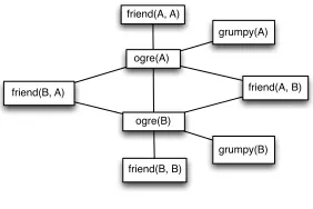
A weighted rule allows truth assignments in which not all instances of the rule hold. Equation 1 above shows sample weighted rules: Friends of ogres tend to be ogres and ogres tend to be grumpy. Suppose we have two constants, Anna (A) and Bob (B). Using these two constants and the predicate symbols in Equation 1, the set of all ground atoms we can construct is:

LA,B={ogre(A),ogre(B),grumpy(A),grumpy(B),friend(A,A),

friend(A,B),friend(B,A),friend(B,B)}

If we only consider models over a domain with these two constants as entities, then each truth assignment toLA,Bcorresponds to a model. MLNs make the assumption of a

one-to-one correspondence between constants in the system and entities in the domain. We discuss the effects of thisdomain closure assumptionbelow.

ogre(A)

ogre(B)

friend(A, B) friend(B, A)

friend(B, B) friend(A, A)

grumpy(A)

grumpy(B)

Figure 1

A sample ground network for a Markov Logic Network.

corresponds to a grounding of a rule. For example, the clique including friend(A,B), ogre(A), and ogre(B) corresponds to the ground rule friend(A,B)∧ogre(A)⇒ogre(B). A variable assignment x in this graph assigns to each node a value of either True or False, so it is a truth assignment (a world). The clique potential for the clique involving friend(A,B), ogre(A), and ogre(B) is exp(1.1) if x makes the ground rule true, and 0 otherwise. This allows for nonzero probability for worlds x in which not all friends of ogres are also ogres, but it assigns exponentially more probability to a world for each ground rule that it satisfies.

More generally, an MLN takes as input a set of weighted first-order formulasF= F1,. . .,Fn and a set C of constants, and constructs an undirected graphical model in

which the set of nodes is the set of ground atoms constructed fromFandC. It computes the probability distributionP(X=x) over worlds based on this undirected graphical model. The probability of a world (a truth assignment)xis defined as:

P(X=x)= 1 Zexp

X

i

wini(x) !

(3)

whereiranges over all formulasFiinF,wi is the weight ofFi,ni(x) is the number of

groundings of Fi that are true in the world x, andZ is the partition function (i.e., it

normalizes the values to probabilities). So the probability of a world increases expo-nentially with the total weight of the ground clauses that it satisfies.

In this article, we useR(for rules) to denote the input set of weighted formulas. In addition, an MLN takes as input an evidence setEasserting truth values for some ground clauses. For example,ogre(A) means that Anna is an ogre. Marginal inference for MLNs calculates the probabilityP(Q|E,R) for a query formulaQ.

Alchemy (Kok et al. 2005) is the most widely used MLN implementation. It is a software package that contains implementations of a variety of MLN inference and learning algorithms. However, developing a scalable, general-purpose, accurate infer-ence method for complex MLNs is an open problem. MLNs have been used for various NLP applications, including unsupervised coreference resolution (Poon and Domingos 2008), semantic role labeling (Riedel and Meza-Ruiz 2008), and event extraction (Riedel et al. 2009).

judges that it plausibly follows from the Text. When using naturally occurring sentences, this is a very challenging task that should be able to utilize the unique strengths of both logic-based and distributional semantics. Here are examples from the SICK data set (Marelli et al. 2014b):

r

T: A man and a woman are walking together through the woods.

H: A man and a woman are walking through a wooded area.

r

T: Nobody is playing the guitar

H: A man is playing the guitar

r

T: A young girl is dancing

H: A young girl is standing on one leg

The SICK (“Sentences Involving Compositional Knowledge”) data set, which we use for evaluation in this article, was designed to foreground particular linguistic phe-nomena but to eliminate the need for world knowledge beyond linguistic knowledge. It was constructed from sentences from two image description data sets, ImageFlickr3 and the SemEval 2012 STS MSR-Video Description data.4_{Randomly selected sentences} from these two sources were first simplified to remove some linguistic phenomena that the data set was not aiming to cover. Then, additional sentences were created as variations over these sentences, by paraphrasing, negation, and reordering. RTE pairs were then created that consisted of a simplified original sentence paired with one of the transformed sentences (generated from either the same or a different original sentence).

We would like to mention two particular systems that were evaluated on SICK. The first is Lai and Hockenmaier (2014), which was the top-performing system at the original shared task. It uses a linear classifier with many hand-crafted features, including alignments, word forms, POS tags, distributional similarity, WordNet, and a unique feature called Denotational Similarity. Many of these hand-crafted features are later incorporated in our lexical entailment classifier, described in Section 5.2. The Denotational Similarity uses a large database of human- and machine-generated image captions to cleverly capture some world knowledge of entailments.

The second system is Bjerva et al. (2014), which also participated in the original SICK shared task, and achieved 81.6% accuracy. The RTE system uses Boxer to parse input sentences to logical form, then uses a theorem prover and a model builder to check for entailment and contradiction. The knowledge bases used are WordNet and PPDB. In contrast with our work, PPDB paraphrases are not translated to logical rules (Section 5.3). Instead, in case a PPDB paraphrase rule applies to a pair of sentences, the rule is applied at the text level before parsing the sentence. Theorem provers and

3http://nlp.cs.illinois.edu/HockenmaierGroup/data.html.

model builders have high precision detecting entailments and contradictions, but low recall. To improve recall, neutral pairs are reclassified using a set of textual, syntactic, and semantic features.

3. System Overview

This section provides an overview of our system’s architecture, using the following RTE example to demonstrate the role of each component:

T: A grumpy ogre is not smiling.

H: A monster with a bad temper is not laughing.

Which in logic are:

T: ∃x.ogre(x)∧grumpy(x)∧ ¬∃y.agent(y,x)∧smile(y)

H: ∃x,y.monster(x)∧with(x,y)∧bad(y)∧temper(y)∧ ¬∃z.agent(z,x)∧

laugh(z).

This example needs the following rules in the knowledge baseKB:

r1: laugh⇒smile

r2: ogre⇒monster

r3: grumpy⇒with a bad temper

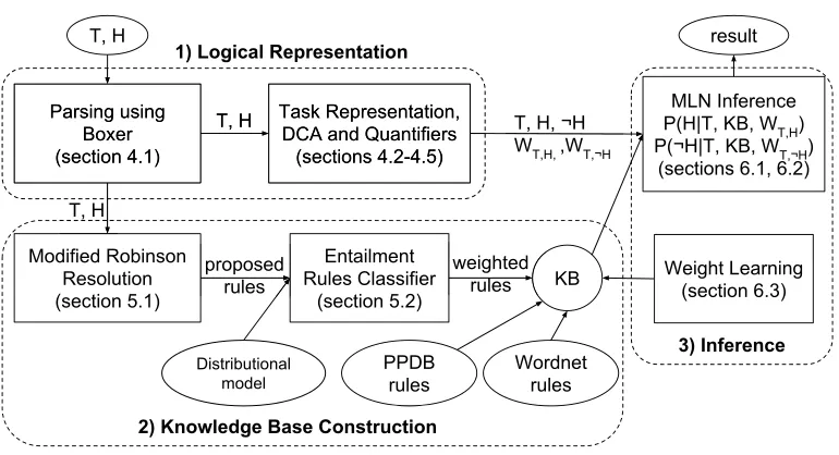
Figure 2 shows the high-level architecture of our system, and Figure 3 shows the MLNs constructed by our system for the given RTE example.

Figure 2

Figure 3

MLNs for the given RTE example. The RTE task is represented as two inferences

P(H|T,KB,WT,H) andP(¬H|T,KB,WT,¬H) (Section 4.1).Dis the set of constants in the domain.

Tandr3are skolemized andskis the skolem function ofr3(Section 4.2).Gis the set of non-False (True or unknown) ground atoms as determined by the CWA (Section 4.3, 6.2).Ais the CWA for the negated part ofH(Section 4.3).D,G,Aare the world assumptionsWT,H( orWT,¬H).r1,r2,r3 are theKB.r1and its weightw1are from PPDB (Section 5.3).r2is from WordNet (Section 5.3). r3is constructed using the Modified Robinson Resolution (Section 5.1), and its weightw3is calculated using the entailment rules classifier (Section 5.2). The resource-specific weights

wppdb,weclassifare learned using weight learning (Section 6.3). Finally, the two probabilities are calculated using MLN inference whereH(or¬H) is the query formula (Section 6.1)

Our system has three main components:

1. Logical Representation (Section 4), where input natural sentencesTand Hare mapped into logic and then used to represent the RTE task as a probabilistic inference problem.

rules, and weighted and added to the inference problem. This is where distributional information is integrated into our system.

3. Inference (Section 6), which uses MLNs to solve the resulting inference problem.

One powerful advantage of using a general-purpose probabilistic logic as a se-mantic representation is that it allows for a highly modular system. Therefore, the most recent advancements in any of the system components, in parsing, in knowledge base resources and distributional semantics, and in inference algorithms, can be easily incorporated into the system.

In the Logical Representation step (Section 4), we map input sentencesTandHto logic. Then, we show how to map the three-way RTE classification (entailing, neutral, or contradicting) to probabilistic inference problems. The mapping of sentences to logic differs from standard first order logic in several respects because of properties of the probabilistic inference system. First, MLNs make the Domain Closure Assumption (DCA), which states that there are no objects in the universe other than the named constants (Richardson and Domingos 2006). This means that constants need to be explicitly introduced in the domain in order to make probabilistic logic produce the expected inferences. Another representational issue that we discuss is why we should make the closed-world assumption, and its implications on the task representation.

In the Knowledge Base Construction stepKB(Section 5), we collect inference rules from a variety of sources. We add rules from existing databases, in particular WordNet (Princeton University 2010) and PPDB (Ganitkevitch, Van Durme, and Callison-Burch 2013). To integrate distributional semantics, we use a variant of Robinson resolution to align the TextTand the HypothesisH, and to find the difference between them, which we formulate as an entailment rule. We then train a lexical and phrasal entailment classifier to assess this rule. Ideally, rules need be contextualized to handle polysemy, but we leave that to future work.

In the Inference step (Section 6), automated reasoning for MLNs is used to per-form the RTE task. We implement an MLN inference algorithm that directly sup-ports querying complex logical formula, which is not supported in the available MLN tools (Beltagy and Mooney 2014). We exploit the closed-world assumption to help reduce the size of the inference problem in order to make it tractable (Beltagy and Mooney 2014). We also discuss weight learning for the rules in the knowledge base.

4. Logical Representation

The first component of our system parses sentences into logical form and uses this to represent the RTE problem as MLN inference. We start with Boxer (Bos 2008), a rule-based semantic analysis system that translates a CCG parse into a logical form. The formula

∃x,y,z.ogre(x)∧agent(y,x)∧love(y)∧patient(y,z)∧princess(z) (4)

themselves. Their semantics derives from the knowledge baseKBwe build in Section 5. The rest of this section discusses how we adapt Boxer output for MLN inference.

4.1 Representing Tasks as Text and Query

Representing Natural Language Understanding Tasks.In our framework, a language-understanding task consists of atextand aquery, along with aknowledge base. The text describes some situation or setting, and the query in the simplest case asks whether a particular statement is true of the situation described in the text. The knowledge base encodes relevant background knowledge: lexical knowledge, world knowledge, or both. In the textual entailment task, the text is the TextT, and the query is the Hypothesis H. The sentence similarity (Semantic Textual Similarity; STS) task can be described as two text/query pairs. In the first pair, the first sentence is the text and the second is the query, and in the second pair the roles are reversed (Beltagy, Erk, and Mooney 2014). In question answering, the input documents constitute the text and the query has the formH(x) for a variablex; and the answer is the entityesuch thatH(e) has the highest probability given the information inT.

In this article, we focus on the simplest form of text/query inference, which applies to both RTE and STS: Given a textTand queryH, does the text entail the query given the knowledge baseKB? In standard logic, we determine entailment by checking whether T∧KB⇒H. (Unless we need to make the distinction explicitly, we overload notation and use the symbolTfor the logical form computed for the text, andHfor the logical form computed for the query.) The probabilistic version is to calculate the probability P(H|T,KB,WT,H), whereWT,H is a world configuration, which includes the size of the

domain. We discussWT,H in Sections 4.2 and 4.3. Although we focus on the simplest

form of text/query inference, more complex tasks such as question answering still have the probabilityP(H|T,KB,WT,H) as part of their calculations.

Representing Textual Entailment.RTE asks for a categorical decision between three categories: entailment, contradiction, and neutral. A decision about entailment can be made by learning a threshold on the probability P(H|T,KB,WT,H). To

differen-tiate between contradiction and neutral, we additionally calculate the probability P(¬H|T,KB,WT,¬H). IfP(H|T,KB,WT,H) is high andP(¬H|T,KB,WT,¬H) is low, this

in-dicates entailment. The opposite case inin-dicates contradiction. If the two probability values are close, this meansTdoes not significantly affect the probability ofH, indicat-ing a neutral case. To learn the thresholds for these decisions, we train an SVM classifier with LibSVM’s default parameters (Chang and Lin 2001) to map the two probabilities to the final decision. The learned mapping is always simple and reflects the intuition described here.

4.2 Using a Fixed Domain Size

MLNs compute a probability distribution over possible worlds, as described in Sec-tion 2. When we describe a task as a textT and a queryH, the worlds over which the MLN computes a probability distribution are “mini-worlds,” just large enough to describe the situation or setting given byT. The probability P(H|T,KB,WT,H) then

worlds that possibly describe T.5 _{The use of “mini-worlds” is by necessity, as MLNs} can only handle worlds with a fixed domain size, where “domain size” is the number of constants in the domain. (In fact, this same restriction holds for all current practical probabilistic inference methods, including probabilistic soft logic [Bach et al. 2013].)

Formally, the influence of the set of constants on the worlds considered by an MLN can be described by the Domain Closure Assumption (DCA; Genesereth and Nilsson 1987; Richardson and Domingos 2006): The only models considered for a set F of formulas are those for which the following three conditions hold: (a) Different constants refer to different objects in the domain: (b) the only objects in the domain are those that can be represented using the constant and function symbols inF: and (c) for each functionf appearing inF, the value off applied to every possible tuple of arguments is known, and is a constant appearing inF. Together, these three conditions entail thatthere is a one-to-one relation between objects in the domain and the named constants of F. When the set of all constants is known, it can be used to ground predicates to generate the set of all ground atoms, which then become the nodes in the graphical model. Different constant sets result in different graphical models. If no constants are explicitly introduced, the graphical model is empty (no random variables).

This means that to obtain an adequate representation of an inference problem consisting of a textTand queryH, we need to introduce a sufficient number of constants explicitly into the formula: The worlds that the MLN considers need to have enough constants to faithfully represent the situation inTand not give the wrong entailment for the query H. In what follows, we explain how we determine an appropriate set of constants for the logical-form representations ofTandH. The domain size that we determine is one of the two components of the parameterWT,H.

Skolemization. We introduce some of the necessary constants through the well-known technique ofskolemization(Skolem 1920). It transforms a formula∀x1. . .xn∃y.F

to∀x1. . .xn.F∗, whereF∗is formed fromFby replacing all free occurrences ofyinFby

a termf(x1,. . .,xn) for a new function symbolf. Ifn=0,f is called aSkolem constant,

otherwise aSkolem function. Although skolemization is a widely used technique in first-order logic, it is not frequently used in probabilistic logic because many applica-tions do not require existential quantifiers.

We use skolemization on the text T (but not the query H, as we cannot assume a priori that it is true). For example, the logical expression in Equation (4), which represents the sentenceT: An ogre loves a princess, will be skolemized to:

ogre(O)∧agent(L,O)∧love(L)∧patient(L,N)∧princess(N) (5)

whereO,L,Nare Skolem constants introduced into the domain.

Standard skolemization transforms existential quantifiers embedded under uni-versal quantifiers to Skolem functions. For example, for the text T: All ogres snore and its logical form∀x.ogre(x)⇒ ∃y.agent(y,x)∧snore(y), the standard skolemization is ∀x.ogre(x)⇒agent(f(x),x)∧snore(f(x)). Per condition (c) of the DCA, if a Skolem function appeared in a formula, we would have to know its value for any constant in the domain, and this value would have to be another constant. To achieve this, we introduce

a new predicateSkolemf instead of each Skolem functionf, and for every constant that

is anogre, we add an extra constant that is alovingevent. The example then becomes:

T:∀x.ogre(x)⇒ ∀y.Skolemf(x,y)⇒agent(y,x)∧snore(y)

If the domain contains a singleogre O1, then we introduce a new constant C1 and an atomSkolemf(O1,C1) to state that the Skolem function f maps the constant O1 to the constantC1.

Existence. But how would the domain contain anogre O1 in the case of the text T:

All ogres snore,∀x.ogre(x)⇒ ∃y.agent(y,x)∧snore(y)? Skolemization does not introduce any variables for the universally quantifiedx. We still introduce a constantO1 that is anogre. This can be justified by pragmatics because the sentence presupposes that there are, in fact,ogres(Strawson 1950; Geurts 2007). We use the sentence’s parse to identify the universal quantifier’s restrictor and body, then introduce entities representing the restrictor of the quantifier (Beltagy and Erk 2015). The sentenceT: All ogres snore ef-fectively changes toT: All ogres snore, and there is an ogre. At this point, skolemization takes over to generate a constant that is anogre. Sentences likeT: There are no ogresis a special case: For such sentences, we do not generate evidence of anogre. In this case, the non-emptiness of the domain is not assumed because the sentence explicitly negates it.

Universal Quantifiers in the Query. The most serious problem with the DCA is that it affects the behavior of universal quantifiers in the query. Suppose we know thatT: Shrek is a green ogre, represented with skolemization asogre(SH)∧green(SH). Then we can conclude thatH: All ogres are green, because by the DCA we are only considering models with this single constant, which we know is both anogreandgreen. To address this problem, we again introduce new constants.

We want a queryH: All ogres are greento be judged true iff there is evidence that allogreswill begreen, no matter how manyogresthere are in the domain. SoHshould follow fromT2: All ogres are greenbut not fromT1: There is a green ogre. Therefore we introduce a new constant Dfor the query and assert ogre(D) to test if we can then conclude thatgreen(D). The new evidenceogre(D) prevents the query from being judged true givenT1. GivenT2, the newogre Dwill be inferred to be green, in which case we take the query to be true. Again, with a query such asH: There are no ogres, we do not generate any evidence for the existence of anogre.

4.3 Setting Prior Probabilities

Suppose we have an empty textT, and the queryH: A is an ogre, whereAis a constant in the system. Without any additional information, the worlds in whichogre(A) is true are going to be as likely as the worlds in which the ground atom is false, soogre(A) will have a probability of 0.5. So without any textT, ground atoms have a prior probability in MLNs that is not zero. This prior probability depends mostly on the size of the setF of input formulas. The prior probability of an individual ground atom can be influenced by a weighted rule, for example,ogre(A)| −3, with a negative weight, sets a low prior probability onAbeing an ogre. This is the second group of parameters that we encode inWT,H: weights on ground atoms to be used to set prior probabilities.

P(H|T,KB,WT,H). However, how useful this conditional probability is as an indication of

entailment depends on the prior probability ofH,P(H|KB,WT,H). For example, ifHhas

a high prior probability, then a high conditional probabilityP(H|T,KB,WT,H) does not

add much information because it is not clear if the probability is high becauseTreally entailsH, or because of the high prior probability ofH. In practical terms, we would not want to say that we can conclude fromT: All princesses snorethatH: There is an ogrejust because of a high prior probability for the existence of ogres.

To solve this problem and make the probabilityP(H|T,KB,WT,H) less sensitive to

P(H|KB,WT,H), we pick a particularWT,H such that the prior probability ofHis

approx-imately zero,P(H|KB,WT,H)≈0, so that we know that any increase in the conditional

probability is an effect of addingT. For the task of RTE, where we need to distinguish entailment, neutral, and contradiction, this inference alone does not account for contra-dictions, which is why an additional inferenceP(¬H|T,KB,WT,¬H) is needed.

For the rest of this section, we show how to set the world configurations WT,H

such thatP(H|KB,WT,H)≈0 by enforcing the closed-world assumption (CWA). This is

the assumption that all ground atoms have very low prior probability (or are false by default).

Using the CWA to Set the Prior Probability of the Query to Zero. The CWA is the assumption that everything is false unless stated otherwise. We translate it to our probabilistic setting as saying that all ground atoms have very low prior probability. For most queries H, setting the world configurationWT,H such that all ground atoms

have low prior probability is enough to achieve thatP(H|KB,WT,H)≈0 (not for negated

Hs, and this case is discussed subsequently). For example,H: An ogre loves a princess, in logic is:

H:∃x,y,z.ogre(x)∧agent(y,x)∧love(y)∧patient(y,z)∧princess(z)

Having low prior probability on all ground atoms means that the prior probability of this existentially quantifiedHis close to zero.

We believe that this set-up is more appropriate for probabilistic natural language entailment for the following reasons. First, this aligns with our intuition of what it means for a query to follow from a text: thatHshould be entailed byTnot because of general world knowledge. For example, ifT: An ogre loves a princess, andH: Texas is in the USA, then althoughHis true in the real world,Tdoes not entailH. Another example: T: An ogre loves a princess,H: An ogre loves a green princess, again,T does not entailH because there is no evidence that theprincessisgreen, in other words, the ground atom green(N) has very low prior probability.

The third reason is computational efficiency. As discussed in Section 2, Markov Logic Networks first compute all possible groundings of a given set of weighted formu-las, which can require significant amounts of memory. This is particularly striking for problems in natural language semantics because of long formulas. Beltagy and Mooney (2014) show how to utilize the CWA to address this problem by reducing the number of ground atoms that the system generates. We discuss the details in Section 6.2.

Setting the Prior Probability of Negated H to Zero.Although using the CWA is enough to setP(H|KB,WT,H)≈0 for mostHs, it does not work fornegated H(negation is part of

H). Assuming that everything is false by default and that all ground atoms have very low prior probability (CWA) means that all negated queriesHare true by default. The result is that all negatedHare judged entailed regardless ofT. For example,T: An ogre loves a princesswould entailH: No ogre snores. ThisHin logic is:

H:∀x,y.ogre(x)⇒ ¬(agent(y,x)∧snore(y))

As bothxandyare universally quantified variables inH, we generate evidence of an ogreogre(O) as described in Section 4.2. Because of the CWA,Ois assumed to bedoes not snore, andHends up being true regardless ofT.

To set the prior probability ofHto≈0 and prevent it from being assumed true when Tis just uninformative, we construct a new ruleAthat implements a kind of anti-CWA. Ais formed as a conjunction of all the predicates that were not used to generate evidence before, and arenegatedinH. This ruleAgets a positive weight indicating that its ground atoms have high prior probability. As the ruleAtogether with the evidence generated fromHstates the opposite of the negated parts ofH, the prior probability ofHis low, andHcannot become true unlessTexplicitly negatesA.Tis translated into unweighted rules, which are taken to have infinite weight, and which thus can overcome the finite positive weight ofA. Here is a neutral RTE example,T: An ogre loves a princess, andH: No ogre snores. Their representations are:

T: ∃x,y,z.ogre(x)∧agent(y,x)∧love(y)∧patient(y,z)∧princess(z)

H: ∀x,y.ogre(x)⇒ ¬(agent(y,x)∧snore(y))

E: ogre(O)

A: agent(S,O)∧snore(S)|w=1.5

E is the evidence generated for the universally quantified variables in H, and A is the weighted rule for the remaining negated predicates. The relation between T andH is neutral, as T does not entailH. This means, we wantP(H|T,KB,WT,H)≈0,

but because of the CWA, P(H|T,KB,WT,H)≈1. Adding A solves this problem and

P(H|T,A,KB,WT,H)≈0 becauseHis not explicitly entailed byT.

In case H contains existentially quantified variables that occur in negated predi-cates, they need to be universally quantified inAforHto have a low prior probability. For example,H: There is an ogre that is not green:

H:∃x.ogre(x)∧ ¬green(x)

If one variable is universally quantified and the other is existentially quantified, we need to do something more complex. Here is an example,H: An ogre does not snore:

H:∃x.ogre(x)∧ ¬(∃y.agent(y,x)∧snore(y) )

A:∀v.agent(S,v)∧snore(S)|w=1.5

Notes About How Inference Proceeds with the Rule A Added.IfHis a negated formula that is entailed byT, thenT (which has infinite weight) will contradictA, allowingH to be true. Any weighted inference rules in the knowledge baseKBwill need weights high enough to overcomeA. So the weight ofAis taken into account when computing inference rule weights.

In addition, adding the ruleAintroduces constants in the domain that are necessary for making the inference. For example, takeT: No monster snores, andH: No ogre snores, which in logic are:

T: ¬∃x,y.monster(x)∧agent(y,x)∧snore(y)

H: ¬∃x,y.ogre(x)∧agent(y,x)∧snore(y)

A: ogre(O)∧agent(S,O)∧snore(S)|w=1.5

KB: ∀x.ogre(x)⇒monster(x)

Without the constantsOandSadded by the ruleA, the domain would have been empty and the inference output would have been wrong. The ruleAprevents this problem. In addition, the introduced evidence in A fits the idea of “evidence propagation” men-tioned earlier (detailed in Section 6.2). For entailing sentences that are negated, as in the example here, the evidence propagates from H toT (not fromT to H as in non-negated examples). In the example, the ruleAintroduces an evidence forogre(O) that then propagates from the LHS to the RHS of theKBrule.

4.4 Textual Entailment and Coreference

The adaptations of logical form that we have discussed so far apply to any natural language understanding problem that can be formulated as text/query pairs. The adaptation that we discuss now is specific to textual entailment. It concerns coreference between text and query.

For these examples, here are the logical formulas with coreference in the updated

¬H:

T:∃x.ogre(x)∧ ¬(∃y.agent(y,x)∧snore(y))

Skolemized T:ogre(O)∧ ¬(∃y.agent(y,O)∧snore(y))

H:∃x,y.ogre(x)∧agent(y,x)∧snore(y)

¬H:¬∃x,y.ogre(x)∧agent(y,x)∧snore(y)

updated¬H:¬∃y.ogre(O)∧agent(y,O)∧snore(y)

Notice how the constantOrepresenting theogreinTis used in theupdated¬Hinstead of the quantified variablex.

We use a rule-based approach to determining coreference betweenTandH, consid-ering both coreference between entities and coreference of events. Two items (entities or events) corefer if they (1) have different polarities, and (2) share the same lemma or share an inference rule. Two items have different polarities in T and H if one of them is embedded under a negation and the other is not. For the example here,ogre inTis not negated, andogre in¬His negated, and both words are the same, so they corefer.

A pair of items inTandHunder different polarities can also corefer if they share an inference rule. In the example ofT: A monster does not snoreandH: An ogre snores, we needmonsterandogreto corefer. For cases like this, we rely on the inference rules found using the modified Robinson resolution method discussed in Section 5.1. In this case, it determines thatmonsterandogreshould be aligned, so they are marked as coreferring. Here is another example:T: An ogre loves a princess,H: An ogre hates a princess. In this case,lovesandhatesare marked as coreferring.

4.5 Using Multiple Parses

In our framework that uses probabilistic inference followed by a classifier that learns thresholds, we can easily incorporate multiple parses to reduce errors due to mispars-ing. Parsing errors lead to errors in the logical form representation, which in turn can lead to erroneous entailments. If we can obtain multiple parses for a textTand query H, and hence multiple logical forms, this should increase our chances of getting a good estimate of the probability ofHgivenT.

The default CCG parser that Boxer uses is C&C (Clark and Curran 2004). This parser can be configured to produce multiple ranked parses (Ng and Curran 2012); however, we found that the top parses we get from C&C are usually not diverse enough and map to the same logical form. Therefore, in addition to the top C&C parse, we use the top parse from another recent CCG parser, EasyCCG (Lewis and Steedman 2014).

Therefore, for a natural language text NT and query NH, we obtain two parses

each, sayST1 andST2 forT and SH1 and SH2 for H, which are transformed to logical forms T1,T2,H1,H2. We now compute probabilities for all possible combinations of representations ofNT and NH: the probability of H1 given T1, the probability of H1 givenT2, and conversely also the probabilities ofH2 given eitherT1 orT2. If the task is textual entailment with the three categories: entailment, neutral, and contradiction, then, as described in Section 4.1, we also compute the probability of¬H1 given either

probabilities as features. In Section 7, we evaluate using C&C alone and using both parsers.

5. Knowledge Base Construction

This section discusses the automated construction of the knowledge base, which in-cludes the use of distributional information to predict lexical and phrasal entailment. This section integrates two aims that are conflicting to some extent, as alluded to in the Introduction. The first is to show that a general-purpose in-depth natural language understanding system based on both logical form and distributional representations can be adapted to perform the RTE task well enough to achieve state-of-the-art re-sults. To achieve this aim, we build a classifier for lexical and phrasal entailment that includes many task-specific features that have proven effective in state-of-the-art systems (Marelli et al. 2014a; Bjerva et al. 2014; Lai and Hockenmaier 2014). The second aim is to provide a framework in which we can test different distributional approaches on the task of lexical and phrasal entailment as a building block in a general textual entailment system. To achieve this second aim, in Section 7 we provide an in-depth ablation study and error analysis for the effect of different types of distributional information within the lexical and phrasal entailment classifier.

Because the biggest computational bottleneck for MLNs is the creation of the network, we do not want to add a large number of inference rules blindly to a given text/query pair. Instead, we first examine the text and query to determine inference rules that are potentially useful for this particular entailment problem. For pre-existing rule collections, we add all possibly matching rules to the inference problem (Sec-tion 5.3). For more flexible lexical and phrasal entailment, we use the text/query pair to determine additionally useful inference rules, then automatically create and weight these rules. We use a variant of Robinson resolution (Robinson 1965) to compute the list of useful rules (Section 5.1), then apply a lexical and phrasal entailment classifier (Section 5.2) to weight them.

Ideally, the weights that we compute for inference rules should depend on the context in which the words appear. After all, the ability to take context into account in a flexible fashion is one of the biggest advantages of distributional models. Un-fortunately the textual entailment data that we use in this article does not lend itself to contextualization—polysemy just does not play a large role in any of the existing RTE data sets that we have used so far. Therefore, we leave this issue to future work.

5.1 Robinson Resolution for Alignment and Rule Extraction

Modified Robinson Resolution.Robinson resolution is a theorem-proving method for testing unsatisfiability that has been used in some previous RTE systems (Bos 2009). It assumes a formula in conjunctive normal form (CNF), a conjunction of clauses, where a clause is a disjunction of literals, and a literal is a negated or non-negated atom. More formally, the formula has the form∀x1,. . .,xn C1∧. . .∧Cm), whereCjis a clause and it

has the formL1∨. . .∨LkwhereLiis a literal, which is an atomaior a negated atom¬ai.

The resolution rule takes two clauses containing complementary literals, and produces a new clause implied by them. Writing a clauseCas the set of its literals, we can formulate the rule as:

C1∪ {L1} C2∪ {L2} (C1∪C2)θ

whereθis a most general unifier ofL1and¬L2.

In our case, we use a variant of Robinson resolution to remove the parts of text Tand queryHthat the two sentences have in common. Instead of one set of clauses, we use two: one is the CNF ofT, the other is the CNF of¬H. The resolution rule is only applied to pairs of clauses where one clause is fromT, the other fromH. When no further applications of the resolution rule are possible, we are left with remainder formulasrT andrH. IfrHcontains the empty clause, thenHfollows fromTwithout inference rules. Otherwise, inference rules need to be generated. In the simplest case, we form a single inference rule as follows. All variables occurring inrTorrHare existentially quantified, all constants occurring in rT or rH are un-skolemized to new universally quantified variables, and we infer the negation ofrHfromrT. That is, we form the inference rule

∀x1. . .xn∃y1. . .ym.rTθ⇒ ¬rHθ

where{y1. . .ym}is the set of all variables occurring inrTorrH,{a1,. . .an}is the set

of all constants occurring inrT orrH and θ is the inverse of a substitutionθ:{a1→

x1,. . .,an→xn}for distinct variablesx1,. . .,xn.

For example, considerT: An ogre loves a princessandH: A monster loves a princess. This gives us the following two clause sets. Note that all existential quantifiers have been eliminated through skolemization. The query is negated, so we obtain five clauses forTbut only one forH.

T:{ogre(A)},{princess(B)},{love(C},{agent(C,A)},{patient(C,B)} ¬H:{¬monster(x),¬princess(y),¬love(z),¬agent(z,x),¬patient(z,y)}

The resolution rule can be applied four times. After that,C has been unified with z (because we have resolvedlove(C) with love(z)),B with y (because we have resolved princess(B) withprincess(y)), andAwith x(because we have resolvedagent(C,A) with agent(z,x)). The formula rT is ogre(A), and rH is ¬monster(A). So the rule that we generate is:

∀x.ogre(x)⇒monster(x)

One important refinement to this general idea is that we need to distinguish content predicates that correspond to content words (nouns, verbs, and adjectives) in the sentences from non-content predicates such as Boxer’s meta-predicatesagent(X,Y). Resolving on non-content predicates can result in incorrect rules—for example, in the case ofT: A person solves a problemandH: A person finds a solution to a problem, in CNF:

T:{person(A)},{solve(B)},{problem(C)},{agent(B,A)},{patient(B,C)} ¬H:{¬person(x),¬find(y),¬solution(z),¬problem(u),¬agent(y,x),¬patient(y,z),

¬to(z,u)}

If we resolvepatient(B,C) withpatient(y,z), we unify the problemCwith the solution z, leading to a wrong alignment. We avoid this problem by resolving on non-content predicates only when they are fully grounded (that is, when the substitution of variables with constants has already been done by some other resolution step involving content predicates).

In this variant of Robinson resolution, we currently do not perform any search, but unify two literalsonlyif they are fully grounded or if the literal inThas auniqueliteral inHthat it can be resolved with, and vice versa. This works for most pairs in the SICK data set. In future work, we would like to add search to our algorithm, which will help produce better rules for sentences with duplicate words.

Rule Refinement.The modified Robinson resolution algorithm gives us one rule per text/query pair. This rule needs postprocessing, as it is sometimes too short (omitting relevant context), and often it combines what should be several inference rules.

In many cases, a rule needs to be extended. This is the case when it only shows the difference between text; and query is too short and needs context to be usable as a distributional rule, for example, in T: A dog is running in the snow, H: A dog is running through the snow, the rule we get is∀x,y.in(x,y)⇒through(x,y). Although this rule is correct, it does not carry enough information to compute a meaningful vector representation for each side. What we would like instead is a rule that infers “run through snow” from “run in snow.”

Remember that the variables x and y were Skolem constants in rT and rH, for example,rT:in(R,S) andrH:through(R,S). We extend the rule by adding the content words that contain the constants R and S. In this case, we add the running event and the snow back in. The final rule is: ∀x,y.run(x)∧in(x,y)∧snow(y)⇒run(x)∧

through(x,y)∧snow(y).

In some cases, however, extending the rule adds unnecessary complexity. However, we have no general algorithm for when to extend a rule, which would have to take context into account. At this time, we extend all rules as described here. As discussed next, the entailment rules subsystem can itself choose to split long rules, and it may choose to split these extended rules again.

andpatient(y). If any of the splits has more than one verb, we split it again, where each new split contains one verb and its arguments.

After that, we create new rules that link any part ofrTto any part ofrHwith which it has at least one variable in common. So, for our example, we obtain∀x heal(x)⇒help(x) and∀y man(y)⇒patient(y).

There are cases where splitting the rule does not work, for example, withA person, who is riding a bike⇒ A biker. Here, splitting the rule and usingperson⇒ biker loses crucial context information. So we do not perform those additional splits at the level of the logical form, though the entailment rules subsystem may choose to do further splits.

Rules as Training Data.The output from the previous steps is a set of rules{r1,...,rn}

for each pair T and H. One use of these rules is to test whether T probabilistically entailsH. But there is a second use, too: The lexical and phrasal entailment classifier that we describe below is a supervised classifier, which needs training data. So we use the training part of the SICK data set to create rules through modified Robinson resolution, which we then use to train the lexical and phrasal entailment classifier. For simplicity, we translate the Robinson resolution rules into textual rules by replacing each Boxer predicate with its corresponding word.

Computing inference-rule training data from RTE data requires deriving labels for individual rules from the labels on RTE pairs (entailment, contradiction, and neutral). The entailment cases are the most straightforward. Knowing thatT∧r1∧...∧rn⇒H,

then it must be that allriare entailing. We automatically label allriof the entailing pairs

as entailing rules.

For neutral pairs, we know thatT∧r1∧...∧rn;H, so at least one of theriis

non-entailing. We experimented with automatically labeling allrias non-entailing, but that

adds much noise to the training data. For example, ifT: A man is eating an appleandH: A guy is eating an orange, then the ruleman⇒guyis entailing, but the ruleapple⇒orange is non-entailing. So we automatically compare therifrom a neutral pair to the entailing

rules derived from entailing pairs. All rulesri found among the entailing rules from

entailing pairs are assumed to be entailing (unlessn=1, that is, unless we only have one rule), and all other rules are assumed to be non-entailing. We found that this step improved the accuracy of our system. To further improve the accuracy, we performed a manual annotation of rules derived from neutral pairs, focusing only on the rules that do not appear in entailing. We labeled rules as either entailing or non-entailing. From around 5,900 unique rules, we found 737 to be entailing. In future work, we plan to use multiple instance learning (Dietterich, Lathrop, and Lozano-Perez 1997; Bunescu and Mooney 2007) to avoid manual annotation; we discuss this further in Section 8.

For contradicting pairs, we make a few simplifying assumptions that fit almost all such pairs in the SICK data set. In most of the contradiction pairs in SICK, one of the two sentencesTorHis negated. For pairs whereTorHhas a negation, we assume that this negation is negating the whole sentence, not just a part of it. We first consider the case whereTis not negated, andH=¬Sh. AsTcontradictsH, it must hold thatT⇒ ¬H,

so T⇒ ¬¬Sh, and henceT⇒Sh. This means that we just need to run our modified

Robinson resolution with the sentencesTandShand label all resultingrias entailing.

Next we consider the case whereT=¬St andHis not negated. AsTcontradicts

H, it must hold that¬St⇒ ¬H, soH⇒St. Again, this means that we just need to run

the modified Robinson resolution withHas the “Text” andStas the “Hypothesis” and

label all resultingrias entailing.

emptyandfullare antonyms. As before, we run the modified Robinson resolution with TandHand obtain the resultingri. Similar to the neutral pairs, at least one of theriis a

contradictory rule, whereas the rest could be entailing or contradictory rules. As for the neutral pairs, we take a rulerito be entailing if it is among the entailing rules derived

so far. All other rules are taken to be contradictory rules. We did not do the manual annotation for these rules because they are few.

5.2 The Lexical and Phrasal Entailment Rule Classifier

After extracting lexical and phrasal rules using our modified Robinson resolution (Section 5.1), we use several combinations of distributional information and lexical resources to build a lexical and phrasal entailment rule classifier (entailment rule

classifierfor short) for weighting the rules appropriately. These extracted rules create

an especially valuable resource for testing lexical entailment systems, as they contain a variety of entailment relations (hypernymy, synonymy, antonymy, etc.), and are actually useful in an end-to-end RTE system.

We describe the entailment rule classifier in multiple parts. In Section 5.2.1, we overview a lexical entailment rule classifier, which only handles single words. Section 5.2.2 describes the lexical resources used. In Section 5.2.3, we describe how our previous work in supervised hypernymy detection is used in the system. In Section 5.2.4, we describe the approaches for extending the classifier to handle phrases.

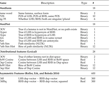
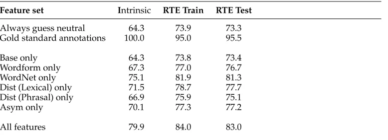
5.2.1 Lexical Entailment Rule Classifier.We begin by describing the lexical entailment rule classifier, which only predicts entailment between single words, treating the task as a supervised classification problem, given the lexical rules constructed from the modified Robinson resolution as input. We use numerous features that we expect to be predictive of lexical entailment. Many were previously shown to be successful for the SemEval 2014 Shared Task on lexical entailment (Marelli et al. 2014a; Bjerva et al. 2014; Lai and Hockenmaier 2014). Altogether, we use four major groups of features, as summarized in Table 1 and described in detail here.

Wordform Features.We extract a number of simple features based on the usage of the LHS and RHS in their original sentences. We extract features for whether the LHS and RHS have the same lemma, same surface form, same POS, which POS tags they have, and whether they are singular or plural. Plurality is determined from the POS tags.

WordNet Features.We use WordNet 3.0 to determine whether the LHS and RHS have known synonymy, antonymy, hypernymy, or hyponymy relations. We disambiguate between multiple synsets for a lemma by selecting the synsets for the LHS and RHS that minimize their path distance. If no path exists, we choose the most common synset for the lemma. Path similarity, as implemented in the Natural Language Toolkit (Bird, Klein, and Loper 2009), is also used as a feature.

Distributional Features. We measure distributional similarity in two distributional spaces, one which models topical similarity (bag of words; BoW), and one which models syntactic similarity (Dependency; Dep). We use cosine similarity of the LHS and RHS in both spaces as features.

Table 1

List of features in the lexical entailment classifier, along with types and counts.

Name Description Type #

Wordform 18

Same word Same lemma, surface form Binary 2

POS POS of LHS, POS of RHS, same POS Binary 10 Sg/Pl Whether LHS/RHS/both are singular/plural Binary 6

WordNet 18

OOV True if a lemma is not in WordNet, or no path exists Binary 1

Hyper True if LHS is hypernym of RHS Binary 1

Hypo True if RHS is hypernym of LHS Binary 1

Syn True if LHS and RHS is in same synset Binary 1

Ant True if LHS and RHS are antonyms Binary 1

Path Sim Path similarity (NLTK) Real 1

Path Sim Hist Bins of path similarity (NLTK) Binary 12

Distributional features (Lexical) 28

OOV True if either lemma not in dist space Binary 2 BoW Cosine Cosine between LHS and RHS in BoW space Real 1 Dep Cosine Cosine between LHS and RHS in Dep space Real 1

BoW Hist Bins of BoW Cosine Binary 12

Dep Hist Bins of Dep Cosine Binary 12

Asymmetric Features (Roller, Erk, and Boleda 2014) 600

Diff LHS dep vector−RHS dep vector Real 300

DiffSq RHS dep vector−RHS dep vector, squared Real 300

to be entailing than words that are moderately similar (0.70–0.89). This is because the most highly similar words are likely to be cohyponyms.

5.2.2 Preparing Distributional Spaces.As described in the previous section, we use dis-tributional semantic similarity as features for the entailment rules classifier. Here we describe the preprocessing steps to create these distributional resources.

Corpus and Preprocessing. We use the BNC, ukWaC, and a 2014-01-07 copy of Wikipedia. All corpora are preprocessed using the Stanford CoreNLP parser. We collapse particle verbs into a single token, and all tokens are annotated with a (short) POS tag so that the same lemma with a different POS is modeled separately. We keep only content words (NN, VB, RB, JJ) appearing at least 1,000 times in the corpus. The final corpus contains 50,984 types and roughly 1.5B tokens.

Figure 4

Distribution of entailment relations on lexical items by cosine. Highly similar pairs (0.90–0.99) are less likely entailing than moderately similar pairs (0.70–0.89).

Dependency Vectors.We extract(lemma/POS, relation, context/POS)tuples from each of the Stanford Collapsed CC Dependency graphs. We filter tuples with lemmas not in our 51k chosen types. Following Baroni and Lenci (2010), we model inverse relations and mark them separately. For example, “red/JJ car/NN” will generate tuples for both (car/NN, amod, red/JJ)and(red/JJ, amod−1, car/NN). After extracting tuples, we discard all but the top 100k(relation, context/POS)pairs and build a vector space usinglemma/POS as rows, and(relation, context/POS)as columns. The matrix is transformed with Positive Pointwise Mutual Information, and reduced to 300 dimensions using Singular Value Decomposition (SVD). We do not vary these parameters, but chose them as they per-formed best in prior work (Roller, Erk, and Boleda 2014).

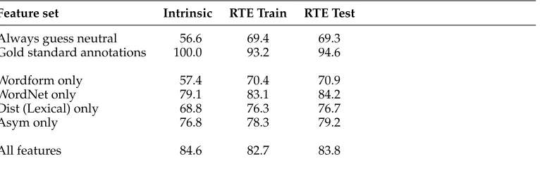
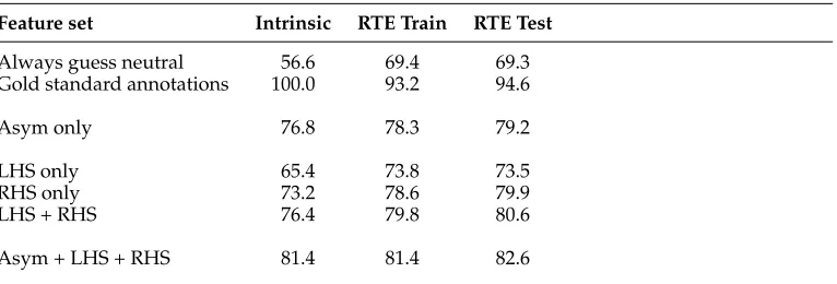
5.2.3 Asymmetric Entailment Features.As an additional set of features, we also use the representation previously utilized by the asymmetric, supervised hypernymy classifier described by Roller, Erk, and Boleda (2014). Previously, this classifier was only used on artificial data sets, which encoded specific lexical relations, like hypernymy, co-hyponymy, and meronymy. Here, we use its representation to encode just the three general relations: entailment, neutral, and contradiction.

The asymmetric features take inspiration from Mikolov, Yih, and Zweig (2013), who found that differences between distributional vectors often encode certain linguistic regularities, like king~ −man~ +woman~ ≈queen~ . In particular the asymmetric classifier uses two sets of features,<f,g>, where:

fi(LHS,RHS)=LHS~ i−RHS~ i

gi(LHS,RHS)=fi2

that is, the vector difference between the LHS and the RHS, and this difference vector squared. Both feature sets are extremely important to strong performance.

outperform word embeddings generated by the Skip-gram procedure. We do not use both spaces, because of the large number of features this creates.

Recently, there has been considerable work in detecting lexical entailments using only distributional vectors. The classifiers proposed by Fu et al. (2014), Levy et al. (2015), and Kruszewski, Paperno, and Baroni (2015) could have also been used in place of these asymmetric features, but we reserve evaluations of these models for future work.

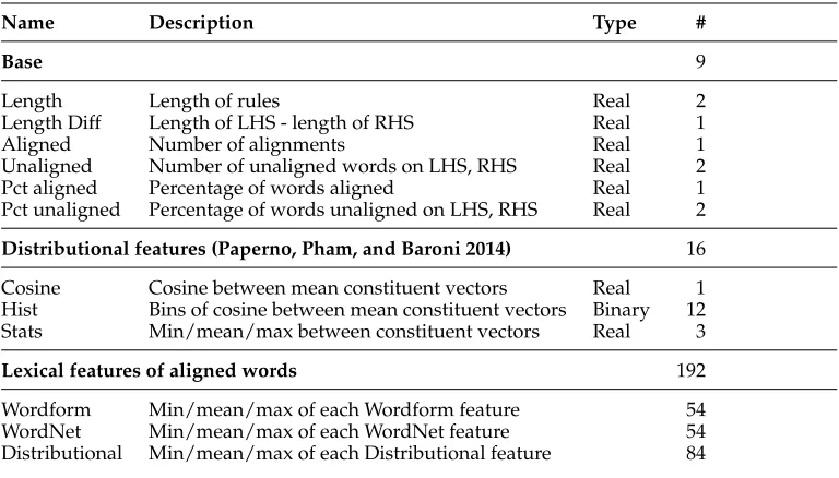
5.2.4 Extending Lexical Entailment to Phrases. The lexical entailment rule classifier de-scribed in previous sections is limited to only simple rules, where the LHS and RHS are both single words. Many of the rules generated by the modified Robinson res-olution are actually phrasal rules, such as little boy → child, or running → moving quickly. In order to model these phrases, we use two general approaches: First, we use a state-of-the-art compositional model, in order to create vector representations of phrases, and then include the same similarity features described in the previous section. The full details of the compositional distributional model are described in Section 5.2.5.

In addition to a compositional distributional model, we also used a simple, greedy word aligner, similar to the one described by Lai and Hockenmaier (2014). This aligner works by finding the pair of words on the LHS and RHS that are most similar in a distributional space, and marking them as “aligned.” The process is repeated until at least one side is completely exhausted. For example, “red truck→ big blue car,” we would align “truck” with “car” first, then “red” with “blue,” leaving “big” un-aligned.

After performing the phrasal alignment, we compute a number of base features, based on the results of the alignment procedure. These include values like the length of the rule, the percent of words unaligned, and so forth. We also compute all of the same features used in the lexical entailment rule classifier (Wordform, WordNet, Distributional) and compute their min/mean/max across all the alignments. We do not include the asymmetric entailment features as the feature space then becomes extremely large. Table 2 contains a listing of all phrasal features used.

5.2.5 Phrasal Distributional Semantics. We build phrasal distributional space based on the practical lexical function model of Paperno, Pham, and Baroni (2014). We again use as the corpus a concatenation of BNC, ukWaC, and English Wikipedia, parsed with the Stanford CoreNLP parser. We focus on five types of dependency labels (amod, nsubj, dobj, pobj, acomp) and combine the governor and dependent words of these dependencies to form adjective–noun, subject–verb, verb–object, preposition–noun, and verb–complement phrases respectively. We only retain phrases where both the governor and the dependent are among the 50K most frequent words in the corpus, resulting in 1.9 million unique phrases. The co-occurrence counts of the 1.9 million phrases with the 20K most frequent neighbor words in a 2-word window are converted to a Positive Pointwise Mutual Information matrix, and reduced to 300 dimensions by performing SVD on a lexical space and applying the resulting representation to the phrase vectors, normalized to length 1.