Non-Linear Restoration from a Single Frame Super Resolution Using Pearson Type VII Density

Non-Linear Restoration from a Single Frame

Super Resolution Using Pearson Type VII

Density

Sakinah Ali Pitchay

Abstract—Super-resolution seeks to recover a high resolution image from one or more low resolution im-ages. It is an ill-posed problem, with no consensus how best to devise image models that can both im-pose smoothness and preserve the edges in the image. Here we investigate the use of prior based on Pearson type VII density integrated with a Markov Random Field (MRF) model. We formulate two different ver-sions, one that acts on the pixel level and another one that acts on the entire image. Having a single down-sampled and noisy version of low resolution frame, we aim to obtain the high resolution image. We compare the state of the art of image priors in super resolu-tion applicaresolu-tion and we discover that our image prior Pearson-MRF achieves the best performance in terms of qualitative measurement.

Keywords: single-frame super-resolution, Pearson type VII, MRF model

1

Introduction

Super-resolution seeks to generate a high resolution im-age from one or more low resolution imim-ages. The lim-itations of the capturing source often allow the loss of resolution including the shifting, rotation, blur and down-sampling. Moreover, the capturing process instigates ad-ditive noise that causes it is not sufficiently to sample the scene adequately. Often the observed frames are de-ficient or noisy, which makes this problem ill-posed and possibly under-determined too. Thus, extra knowledge is vital to acquire an adequate solution and well-known as image prior. Employing the probabilistic model based framework, this extra information may be specified as a prior distribution on the salient statistics that images are known to have. The two main criterions are apparently contrary each other: local smoothness and the existence of edges. Hence the requirement of a good image prior is demanding.

The former prior models have been proposed in the

lit-∗_{Sakinah Ali Pitchay is with the Faculty of Science and}

Technol-ogy, Islamic Science University of Malaysia (USIM), Bandar Baru Nilai, 71800 Nilai, Negeri Sembilan, Malaysia. Currently she is a PhD student in School of Computer Science, The University of Birmingham, United Kingdom. (email:[email protected] / [email protected]).

erature, yet with no substantiation. Gaussian Markov Random Fields represent a common choice for its compu-tational tractability. The Huber-MRF is prominent since it is more robust but still convex and works in [5, 6, 7] are considered to be the state of the art approach.

In our previous paper [3], we proposed a robust den-sity, the univariate version of Pearson type VII formu-lated as Markov Random Field(MRF) in super resolution approach. Previously, the comparison with the existing image priors are concentrating on compressive matrices transformation. Due of curiosity, we formulated and ex-amined the multivariate of Pearson type VII and compare it with the state of the art approach using the classical super resolution technique. This density is formerly used as robust density estimation in [1] as alternative to the t-mixtures and in stock market modelling [2]. The re-mainder of the paper is organised as follow. In Section 2, we describe the problem formally including how to es-timate the high resolution image. Section 3 presents the image prior that we investigate. Section 4 presents our proposed solution and Section 5 details the experimental results and their analysis. Finally, Section 6, concludes the paper.

2

Framework of Image Super Resolution

2.1

Observation Model

The high resolution image ofN =r×c pixel intensities will be vectorised and denoted asz. This image suffers a quite complicated transformation into a low-resolution frame includes blur and down-sampled. We adopt a linear model to express this transformation which, although it is not completely accurate, it has worked well in many previous studies on super-resolution [4, 5, 7]. Denoting the low resolution frame byy in a vectorised form, and the linear transform that takesz into y by W where it is a stack of trasformation matrices into a single matrix W. We expand the forward model as the following:

a linear blur operation and the down-sampling by row and column operator. η is a vector that represents an additive noise, assumed to be Gaussian with zero-mean and σ2 variance. To make the problem more challeng-ing, an additive noise is contaminated to the blurred and down-sampled image.

2.2

The Joint Model

The overall model is the joint model of the observations

yand the unknownsz. Using these, we have joint prob-ability

P r(y,z) =P r(y|z)P r(z) (2) where the first term is the observation model, the second term is the image prior model. Hence we have for the first term in (2):

P r(y|z)∝exp

− 1

2σ2(y−W z)

T_{(y−W z) (3)}

This is also called the model likelihood, because it ex-presses how likely it is that a given z produced the ob-served y through the transformation W. The second term of (2) will be instantiated with either one of the im-age priors discussed in Section 3. To achieve our goal, we need to ’invert’ the causality described by our model, to infer the latent variableszfrom the observed variablesy.

2.3

Inverting the model to estimate

z

We can invert the causality encoded in a probabilistic model by the use of Bayes’ rule.

P r(z|y) = P r(y|z)P r(z)

P r(y) (4) This is called theposterior probability ofzgiven the ob-served datay. Eq. (4) says that, the probability that z is the hidden image that gave rise to what we observed, i.e. y, is proportional to the likelihood that thiszfits the data y and the probability that this bunch of N inten-sity values, i.e. the vectorz, actually ’looks like’ a valid image. Note that the latter is desperately needed in un-derdetermined systems, since there are infinitely many vectorsz that fit the data.

2.4

Maximum

A

Posteriori

Inference

through Optimisation

To obtain the most probable estimate ofzthat conforms to our model and data, we need to maximise (4) as a function of z. Observe that, the denominator, P r(y) does not depend on z. Hence, the maximum value of the fraction (4) occurs for exactly the samez for which the maximum of the numerator does. That is, the most probable estimate is given by:

ˆ

z = arg max z

P r(y|z)P r(z)

P r(y) (5) = arg max

z P r(y|z)P r(z) (6)

Further, this maximisation is also equivalent to maximis-ing the logarithm in the right hand side, since the log-arithm is a monotonic increasing function. We can also turn the maximisation into minimisation, by flipping the signs, as in the following equivalent rewriting:

ˆ

z= arg min

z {−log[P r(y|z)]−log[P r(z)]} (7) In words, the most probable high resolution image is the one for which the negative log of the joint probability model takes its minimum value. Thus, our problem is now solvable by performing this minimisation. The ex-pression to be minimised, i.e. the negative log of the joint probability model may be interpreted as an error objective, and shall be denoted as:

Obj(z) =−log[P r(y|z)]−log[P r(z)] (8) The most probable estimate is the ˆz that has highest probability in the model. Equivalently the one that achieves the lowest error. Since our model has had two factors (the likelihood or observation model, and the im-age prior), consequently our error-objective also has two terms: the misfit to observed data, and ’penalty’ for vi-olating the smoothness and/or other characteristics en-coded in the prior. By plugging in the functional forms for the observation model and for the various possible priors into (8), we now give the specific form of this ob-jective function below, so the interpretation of the indi-vidual error terms is more evident. We will make use of the following notation, taking the log of eq. (3):

l(z) := −logP r(y|z) +const. (9)

= 1

2σ2(y−W z)

T_{(y−W z) (10)}

3

Prior Image Model: Markov Random

Fields

The main characteristic of any natural image is a local smoothness. That is, the intensities of neighbouring pix-els tend to be very similar. A MRF is a joint distribu-tion over all the pixels on the image that captures spatial dependencies of pixel intensities. A first-order MRF as-sumes that, for any pixel, its intensity depends on the intensities of its closest cardinal neighbours but does not depend on any other pixel of the image. Here we will adopt the 1-st order MRF that conditions each pixel of intensity on its four cardinal neighbours in the following way. For any one pixelzi we define:

P r(zi|z−i) = P r(zi|z4neighb(i)) (11)

= P r(zi−1₄

j∈4neighb(i)

zj) (12)

denoted as 4neighb(i). This is a univariate probability distribution.

Consequently, for the whole image ofN pixels, the MRF represents the joint probability over all the pixels on the image — a multivariate probability distribution.

P r(z) ∝

N

i=1

P r(zi|z4neighb(i)) (13)

=

N

i=1

P r(zi−1₄

j∈4neighb(i)

zj) (14)

The notation ’∝’ means ’proportional to’, i.e. there is a division by a constant that makes the probability den-sity integrate to one. This constant may depend on vari-ous parameters of the actual instantiation of the building block probability densities, but it does not depend onz. Since in this work we only need to estimatez, therefore we can ignore the expression of the normalising constant throughout.

This form of MRF has been previously employed with success in e.g. [4, 5]. Alternatives include the so-called total variation model, employed e.g. in e.g. [7],which is based on image gradients, also quite simple. In [6], an experimental comparison of these two alternatives sug-gests these have comparable performance, the former be-ing slightly superior though.

The simplicity of (14) is also intuitively appealing. One can think of the difference between a pixel intensity and the average intensity of its neighbours, i.e. zi −

1 4

j∈4neighb(i)zj, as afeature. Considering that we want to encode the general smoothness property of images, it is easy to see that this feature is very useful: When-ever this difference is small in absolute value, we have a smooth neighbourhood. Whenever it is large in abso-lute value, we have a discontinuity. Hence, to express smoothness, we just need to instantiate the probability distribution over this feature, i.e. the uni-variate densi-ties in the product (14),P r(zi−14

j∈4neighb(i)zj), with

symmetricdensities around zero, which give high proba-bility to small values. The Gaussian is a good example. In the same time, to allow for a few discontinuities, we need to use heavy tail densities, such as the Huber or the Pearson type VII density.

To simplify notation and it is conveniently to create the symmetricN×N matrixD to encode the above neigh-bourhood structure, with entries:

dij=

⎧ ⎨ ⎩

1 ifi=j;

−1/4 if i and j are neighbours; 0 otherwise.

Then we may write thei-th feature in a vector form, with the aid of thei-th row of this matrix (denotedD_i) as the

following:

zi−1₄

j∈4neighb(i)

zj = N

j=1

dijzj (15)

= Diz (16)

Again, this is thei-th neighbourhood feature of the im-age, and there arei = 1, . . . , N such features on an N -pixel image.

The studies of data visualisation of the neighbour-hood features (Diz) from several natural images are presented

in a histogram. We now turn to instantiate the functional form of the probability densities that describe the shape of the likely values of these features. Figure 1 shows a few examples of observed histograms of these features, from natural images. The probability densities that we employ in our image priors should ideally have similar shapes.

−0.2 0 0.2 0.4 0

500 1000 1500 2000 2500 3000 3500 4000 4500

cameraman

Diz

count

−0.1 0 0.1 0.2 0

500 1000 1500 2000

panda bear

Diz

count

−0.2 0 0.2 0.4 0.6 0

500 1000 1500 2000 2500

ladybug

Diz

count

−0.2 0 0.2 0

500 1000 1500 2000 2500 3000

chamomile flower

Diz

count

Figure 1: Examples of histograms of the distribution of neighbourhood features Diz, i= 1,· · ·, N from natural images.

3.1

Gaussian-

MRF

The Gaussian MRF is the most widely used image prior density. It has the following form:

P r(z) ∝

N

i=1 exp

− 1

2λ(Diz)

2 ₍₁₇₎

= exp

− 1

2λ

N

i=1 (D_iz)2

(18)

whereλis the variance parameter.

3.2

Huber-

MRF

The Huber density is defined with the aid of the Huber function. It takes a threshold parameterδ, specifying the value at which it diverts from being quadratic to being linear. A generic variableuin the definition of this func-tion will be instantiated later as a neighbourhood-feature

Diz within the image prior use.

H(u|δ) =

u2, if|u|< δ

The Huber-MRF prior is then defined in (21) whereλis similar to a variance parameter.

P r(z) ∝

N

i=1 exp

− 1

2λH(Diz|δ)

(20)

= exp

− 1

2λ

N

i=1

H(D_iz|δ)

(21)

4

Pearson Type VII-MRF

4.1

The univariate Pearson Type VII-MRF

The Pearson-MRF made of univariate building blocks: A zero mean univariate Pearson prior, is defined as:

P r(z)∝

N

i=1

(D_iz)2+λ−(1+2ν) ₍₂₂₎

whereν andλcontrol the shape of the distribution.

4.2

The multivariate Pearson Type

VII-MRF

A zero mean multivariate Pearson-MRF density in a generic N-dimensional vector of D_iz, has the following form:

P r(z)∝ _N

i=1

(D_iz)2+λ

−(ν+N

2 )

(23)

4.3

Discussion

on

the

two

versions

of

Pearson-MRF

The version devised in Section 4.1 may be re-garded as having independent Pearson-priors on each neighbourhood-feature. Of course, we ought to point out that the neighbourhood features are not independent in reality. However, since each pixel only depends on four others, it may be a reasonable approximation.

The version gave in section 4.2, in turn, does not allow such independence interpretation. Conversely, this can has the advantage that the spatial dependencies are not broken up, but more reliably accounted for. However, on the downside, the heavy tail behaviour is more advanta-geous to have on the pixel level, i.e., on the distribution of neighbourhood features. Indeed, it is the distribution of neighbourhood features the one in which the edges from the image creates outliers. In turn, the multivariate Pearson-MRF is a density on images. Hence, its heavy tail behaviour would be well suited to account for outly-ing or atypical images. Includoutly-ing both of these versions in our comparison will therefore uncover to us which of these pros or cons are more important for recovering qual-ity high resolution images.

5

Experiments

5.1

Experimental Setting

We present two set of a single frame image super res-olution experiments illustrating the performance of the hyper-parameters and four different images for testing the stability of the parameters found. The LR image is blurred by the unifrom blur matrix of size 3x3, down-sampled by factor 4 and contaminated by standard de-viation of Gaussian noise of 1e-3 and 1e-2. The original image for Exp. 1 is the cameraman, Exp. 2 is the panda bear, Exp. 3 is the chamomile flower and Exp 4 is the ladybug. All are in size 100x100. The initial guess was initialized with Gaussian-MRF with σ2/λ set to 1 and was used as a starting point for the recovery algorithm. We employed a conjugate gradient type method1, which requires the gradient vector of the objectives. All the pixel intensities are scaled to interval [-0.5,0.5].

In our paper [3], we applied the compressive matrix of W to find out how well is the proposed image prior based MRF in comparison with other state of the art priors, and hyper-parameters is manually tuned to acquire the opti-mum mean square error for all methods. Meanwhile in this paper we compare it using the transformation matrix consists of blur and down-sampling, which one of the two version of Pearson works better and does it still good al-though for a different transformation? Secondly how the selection of hyper-parameters of univariate Pearson type VII is determined and how good is the proposed prior in under-determined system where W has [2500,10000] size. For this experiment, we wider the test images and the noise variance as well.

5.2

Hyper-parameters Selection of

Pearson-MRF

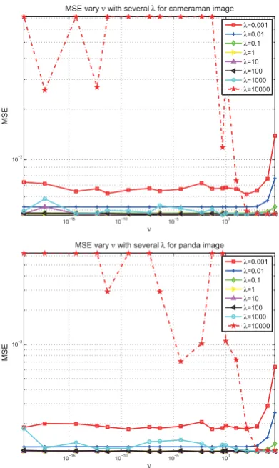
The performance of the image recovery of high resolu-tion is depending on how good selecresolu-tion value of hyper-parameters in image prior. Bad estimation can lead to produce a bad result. Since we are assessing the perfor-mance of both parameters, the recovery algorithm is as-suming knowing the true noise varianceσ2. From the ob-servation using the constructed blur and down-sampling matrix W, we found practical range ofλandν.

The results are presented in Figure 2. Too smallλ(0.001) and ν reduces the effect of prior and the solution ap-proaching the Maximum Likelihood(ML). Whilst too big

λ(10000) will blur the edges. The overall performance of the recovered image is depending strongly on the selec-tion ofλ. We can conclude that theν can be fixed into a practicable range (i.e:1-10) so that the iteration could terminate earlier and theλis found best from 0.1 to 100. Two set of images (cameraman and panda image) are

1_{We made use of the efficient implementation available from}

examined to achieve the best performance. While Fig-ure 3 shows the variation performance varying severalλ. Besides, the performance for several level of noise is in-vestigated using one of the stable range ofν using four different images and the results are presented in Figure 4.

10−15 ₁₀−10 ₁₀−5 ₁₀0

10−2

ν

MSE

MSE vary ν with several λ for cameraman image

λ=0.001

λ=0.01

λ=0.1

λ=1

λ=10

λ=100

λ=1000

λ=10000

10−15 ₁₀−10 ₁₀−5 ₁₀0

10−2

ν

MSE

MSE vary ν with several λ for panda image

λ=0.001

λ=0.01

λ=0.1

λ=1

λ=10

λ=100

λ=1000

λ=10000

Figure 2: Top: Test image of cameraman, bottom: test image of panda are used to inspect the best value of hyper-parameters by computing the MSE performance varying severalλwhere noise variance is 0.001.

5.3

Results

To asses the goodness of the proposed method, Pearson-MRF estimation results are compared with image en-hancement state of the art methods in [4, 5, 7] using the qualitative measurement, mean square error (MSE). The competing image priors are: Gaussian-MRF, a multivari-ate Pearson type VII based MRF and the Huber-MRF. These results are presented in Figure 5 and we can see that the univariate Pearson type VII based MRF can achieve state-of-the-art performance, comparable to the Huber-MRF as well across all noise levels tested while the other priors tested perform worse. Finally we also il-lustrated two recovery set of experiment where the trans-formation matrix consists blur and down-sampling. Here we generated a single frame of high resolution for

under-10−4 ₁₀−3 ₁₀−2 ₁₀−1 ₁₀0 ₁₀1 ₁₀2 ₁₀3 ₁₀4

10−2

λ

MSE

Standard deviation of noise, σ = 0.001 varying several λ

Exp. 1 Exp. 2

Figure 3: MSE measurement varying λ where the ν is fixed to 0.05 and this value is found one of the best from manually search.

0.1 0.2 0.3 0.4 0.5 0.6 0.7 0.8 0.9 1 2

3 4 5 6 7 8 9

x 10−3

λ

MSE

Standard deviation of noise, σ = 0.001

Exp. 1 Exp. 2 Exp. 3 Exp. 4

0.1 0.2 0.3 0.4 0.5 0.6 0.7 0.8 0.9 1 2

3 4 5 6 7

x 10−3

λ

MSE

Standard deviation of noise, σ = 0.01

Exp. 1 Ex.p 2 Exp. 3 Exp. 4

determined system as well in this case. Figure 7 shows the outcome using univariate Pearson type VII based MRF.

0.01 0.02 0.03 0.04 0.05 0.06 0.07 0.08 0.09 0.1 5

6 7 8 9 10 11

x 10−3

σ

MSE

u−PearsonVII MRF m−PearsonVII MRF Huber MRF Gaussian MRF

Figure 5: Comparative MSE performance for under-determined system where W has [2500,10000] and vary-ing several level of noise usvary-ing the best values of hyper-parameter for every image prior. The error bars are over 10 independent trials.

0.01 0.02 0.03 0.04 0.05 0.06 0.07 0.08 0.09 0.1 1

2 3 4 5 6 7 8 9

x 10−3

σ

MSE

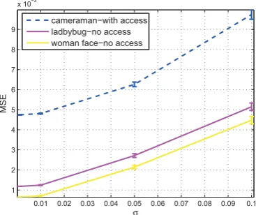
cameraman−with access ladbybug−no access woman face−no access

Figure 6: Comparing the MSE performance of the image with the access to the ground truth image for finding the hyperparameters Pearson type VII baased MRF and us-ing the same value of the optimal found for other images. The error bars are over 10 independent trials over the ran-dom draw of the additive noise and the transformation W consists of blur and down-sampling.

6

Conclusions and Future Work

In this paper we formulated two versions of Pearson-MRF image priors, and conducted a comparative experimental study among these and state of the art methods of image prior from a single noisy version of low resolution im-age. We demonstrate that our proposed prior, univariate Pearson Type VII-MRF is likewise superior with Huber for all level of noise. The recovered image is always con-sistent although it has several local optima and we asses

Ground Truth Low resolution image

Ground Truth Low resolution image Pearson

Figure 7: Left: Ground truth image, blurred and down-sampled image corrupted by additive noise and estimated image using Pearson-MRF from a noisy version of single low-resolution frame. The problem is under-determined system where W[2500,10000] and theσis 0.001.

four different images. Our motivation for Pearson-MRF prior has been the heavy tail property of the Pearson type VII-distribution, which indeed seems to be a good way of preserving the edges too while imposing smooth-ness. We tested this in under-determined systems, using the optimal value under various natural images. Future work is aimed towards recovering from multiple frames and working with multiple scenes for under-determined system and over-determined system as well.

References

[1] J.Sun, A.Kab´an and J.Garibaldi, “Robust Mixture

Mod-eling using the Pearson Type VII Distribution“, Pro.

Int. Joint Conference on Neural Network, 2010, to appear.

http://www.cs.bham.ac.uk/∼axk/PearsonTypeVIIMixture.pdf

[2] Y.Nagahara, “Non-gaussian distribution for stock returns and related stochastic differential equation“,Asia-Pacific Finan-cial MArkets, V3, N2, pp. 121-149, 1996

[3] AKaban and S.A. Pitchay, “Single-frame Image

Super-resolution Using a Pearson Type VII MRF“,Proc. IEEE

In-ternational Workshop on Machine Learning for Signal Pro-cessing, (MLSP 2010)

[4] R. C. Hardie, K. J. Barnard, “Joint MAP Registration and High-Resolution Image Estimation Using a Sequence of

Un-dersampled Images“’, IEEE Trans. Image Processing, V6,

N12, Dec. 1997, pp. 621–633.

[5] H. He and L.P. Kondi, “MAP Based Resolution Enhancement of Video Sequences Using a Huber-Markov Random Field

Image Prior Model“,IEEE Conference of Image Processing,

2003, pp. 933-936.

[6] H. He and L.P. Kondi, “Choice of Threshold of the Huber-Markov Prior in MAP Based Video Resolution

Enhance-ment“,IEEE Electrical and Computer Engineering Canadian

Conference, 2004.

[7] L. C. Pickup, D. P. Capel, S. J. Roberts, A. Zissermann,

“Bayesian Methods for Image Super-Resolution“,The