Abstract—Engineering system can provide value over time in a dynamic environment when system’s components are designed with flexibility. This paper presents a sensitivity-based method to identify where to add flexibility within systems when considering external uncertainty. The sensitivity-based method defines the sensitivity of design variables which are measured by the number of exogenous factors that can directly or indirectly influence them. The relationships of design variables and exogenous factors are represented by directed graph in this paper. In addition, a DFS-based algorithm is proposed to quantitatively and efficiently measure the sensitivity of each design variable when inter-relationship within a system is complex. A case study on the design of a High Speed Rail (HSR) system is used to demonstrate the proposed approach. Results show that the proposed approach can quantitatively identify all the flexible design opportunities. Furthermore, adding flexibility into the selected opportunity will result in significant reduction in the total project’s over long term.
Index Terms—Flexible design opportunities, sensitivity, external uncertainty
I. INTRODUCTION
Flexibility has become an increasingly important design criterion in the system design process for engineering systems that are subject to external uncertainties [1]. Many applications such as water resource systems [2], offshore oil platforms [3], [4], infrastructure systems [5], [6] etc., have shown that system designs with flexible design opportunities can increase the overall performance compared to traditional rigid design process. Therefore, it is not surprising that flexible designs are widely used in many real world applications.
According to [2], [7], flexibility can be considered in two ways: ―on‖ system and ―in‖ system. Flexibility ―on‖ system relates to management decisions. It affects system as a whole component. For example, the flexibility to abandon and expand a project between two decision phases is the source of flexibility ―on‖ system. Flexibility ―on‖ system can be easily incorporated in design. Furthermore, the valuation of flexibility ―on‖ system has been fully investigated in the literature, including methods based on real option analysis. Flexibility ―in‖ system design, on the other hand, refers to the
Manuscript received July 6, 2011
Junfei Hu is a Ph.D. candidate in the Department of Industrial and Systems Engineering, National University of Singapore, Singapore 119260 (e-mail: [email protected])
Kim-Leng Poh is an Associate Professor in the Department of Industrial and Systems Engineering, National University of Singapore, Singapore 119260 (e-mail: [email protected])
ease with which changes can be made in a system due to the influence of factors which are external to the system. Its goal is to make a system adaptable to its environment by incorporating flexibilities within the physical components of system. Recent research on flexibility ―in‖ system has mainly focused on valuation of flexible options based on the assumption that the flexible design opportunities are available a priori (e.g., [8]). However, the identification of flexible design opportunities is also a vital aspect in the system design, since it ensures that all flexible design alternatives are investigated during the design process. In the existing literature, the research on the identification of flexible design opportunities is still limited.
Recently, several methods have been developed to address the problem on identifying where flexibility should be embedded during design process. The existing work can be organized into two categories. The first category is the Design System Matrix (DSM)-based methods. These include change propagation analysis (CPA) [9], sensitivity Design Structure Matrix (sDSM) [10], and Engineering System Matrix (ESM) [11]. The second category employs screening methods. These include the optimization screening method [2], and One-Factor-At-a-Time (OFAT) algorithm [12]. Although these works have attempted to address the issue of identifying flexible design opportunities, they do have some limitations. First of all, all of the DSM-based methods are used to identify insensitive components to design optimal platforms. However, the issues of identifying flexibility design opportunities in system are not clearly dealt with. Secondly, in most of the DSM-based methods, only direct relationships are considered. For example, in [9], the change propagation index of a particular element is measured by comparing the direct change ―in‖ the element and the direct change ―out‖ of the element. The CPA is useful only when one external factor is the change instigator for the whole system. Another example is [10], which introduces a methodology and algorithm for the qualitative identification of platform components. The insensitive platform component is selected only when there is no direct relationship from functional requirement and other design variables to it. The sDSM is suitable only when the direct relationships are easily identified in early design phase. However, in the real world, many external factors such as technical innovation and stakeholder‘s requirements are uncertain and need to be considered together. Furthermore, direct relationships are difficult to identify when there are a large number of design variables, and the inter-relationships between the design
A Sensitivity-based Approach for Identification
of Flexible Design Opportunities in Engineering
System Design
variables are complex. Therefore, considering only the direct relationships is not suitable in most real-world applications.
In this paper, our research focuses on the area of flexibility ―in‖ system. Specifically, we are interested in the problem of identifying where flexibilities should be embedded in engineering system designs. A sensitivity-based approach for identification of flexible design opportunities is proposed. The proposed method identifies flexible design opportunities based on whether the design variables of the system are sensitive to external uncertainties or not. In other words, if the design variable is either directly or indirectly influenced by exogenous factors, it will be considered as a potential flexible design opportunity in design process. A Depth-First-Search (DFS)-based algorithm, which can quantitatively measure the sensitivity of each design variable for engineering system design, is presented.
Our work is inspired by some previous work. Specifically, our work is an extension of DSM-based method; however, it differs from DSM-based methods in several aspects. First of all, our work uses the directed graph to represent the inter-relationships among external factors and design variables in the engineering system. This allows designers to analyze the system in a systematical manner. Secondly, our work identifies both direct and indirect influences from external uncertainties to design variables. Third, it quantitatively measures the sensitivity of design variables. This helps designers to identify which are the most sensitive design variables to external factors. The designers can focus on this set of variables when designing flexible alternatives.
The remainder of the paper is organized as follows. Section 2 presents the sensitivity-based method using directed graphs. Section 3 describes the DFS-based algorithm. Section 4 shows a case study based on the design of a hypothetical High Speed Rail (HSR) system. Section 5 concludes with a summary and suggests future work.
II. SENSITIVITY-BASED METHOD
The sensitivity-based method aims to find the system‘s design variables which are sensitive to exogenous factors. Specifically, it attempts to find the system‘s design variables that need to be changed in order to adapt to the changes of exogenous factors. Those design variables which are identified by the sensitivity-based method are defined as flexible design opportunity in this paper. Identification of flexible design opportunities allows flexibility incorporation in the early phase of the design process making the system adaptable to its environment and provides a good performance in long time horizon. In this section, a measure of sensitivity of design variable is first defined. This measure is then used in the procedure for the identification of flexible design opportunities.
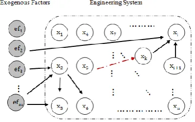
Directed graph is used to present the complex relationships between design variables and exogenous factors in the sensitivity-based method. Fig 1 shows a graph representation of a generic engineering system. Nodes represent design variables, which are within the system boundary. Exogenous factors, which are presented by nodes in Fig 1, account for external uncertainties. The directed arcs in Fig 1 represent the direct influence relationships. For example, the arc between exogenous factor and design variable means that
when the exogenous factor changes, the design variable
needs to be changed accordingly.
[image:2.595.333.533.89.214.2]
Fig 1: Engineering system with complex relationships
In reality, the design variables are not only directly influenced by exogenous factors, but may also be indirectly influenced by exogenous factors through other design variables. For example, in Fig 1, the design variable is directly influenced by exogenous factor . Similarly, the design variable may be indirectly influenced by the exogenous factor though the design variable . This is represented by a path from the exogenous factor to the design variable in Fig 1. This indirect influence means that any change of the exogenous factor may instigate the change of design variable through the perturbation of the design variable . Although indirect influence relationship and direct influence relationship affect engineering system in different ways, both of these relationships are important for the designers. This is because that both of the relationships can instigate the changes of design variables. Therefore, the design variable is sensitive to the exogenous factors by direct or indirect influence relationship.
We define the sensitivity of each design variable in a graphical manner. Consider a system which can be described using n variables X . In addition, exogenous factor of the system is analyzed, according to the future uncertainties EF= . A design variable is said to be sensitive in the neighborhood of a particular exogenous factor under any of the following two situations:
1) Direct influence The design variable is directly influenced by an exogenous factor. In other words, there is an arc from the exogenous factor to the design variable in the directed graph (e.g. );
2) Indirect influence The design variable is indirectly influenced by exogenous factors through another design variable. In other words, there is a path from the exogenous factor to the design variable in the directed graph (e.g. ).
We also define a design variable as being more sensitive, compared to another design variable, when it is influenced by more exogenous factors compared to the other. For example, in Fig 1, there are two paths from factors and to variable . Therefore, the variable is sensitive in the
neighborhood of factors and . Now, for variable
same with variable because variable is only sensitive in
the neighborhood of the two factors and . Therefore, in the sensitivity-based method, the sensitivity of each design variables can be measured by the number of exogenous factors which can affect it. It is not measured by the number of paths from the exogenous factors to a particular design variable.
III. DFS-BASED ALGORITHM
In the previous section, the sensitivity of design variable is defined and quantitatively measured by counting the number of exogenous factors which can affect it. The relationship path from the exogenous factors to the design variables can be easily identified when a system has simple inter-relationships among design variables. However, in most real-world applications, a large number of design variables are usually required and the interconnections among the design variables are usually complex. For example, the sensitivity of the design variables cannot be identified easily when the system as shown in Fig 1 is designed. Specifically, the relationship path from factor to variable is difficult to find. A DFS-based algorithm is presented in this section to efficiently find the entire path from the exogenous factors to a particular design variable. In addition, it also quantitatively calculates the sensitivity of design variables.
The proposed algorithm is based on depth-first search (DFS). DFS is one of the techniques for traversing a graph. It starts at the root and explores as far as possible along each branch before backtracking [13]. Specifically, in this system engineering domain, the algorithm starts at a design variable called n and visits the first child node of n in the graph and goes deeper and deeper until a factor node f is found or until it hits a node that has no children. Then the search backtracks, returning to the most recent node which has not been visited. If a factor node f is found, it shows that there is a path from factor node f to variable node n, and therefore the factor node
f can affect the variable node n. The sensitivity of the variable node n will be incremented by one. After traversing a graph, all factor nodes, which can affect the design variable n will be found.
One of the inputs for the algorithm is the directed graph G,
which was discussed in the previous section. The directed graph G is constructed by using the information provided by the users and historical data. It should be noted that when construct the directed graph G, no arcs should be included from design variable to exogenous factor. This is because that we do not consider the influence of design variable to exogenous factors. The algorithm also involves two lists of nodes. One is a variable list which consists of all elements of design variables and the other one is a factor list which consists of all exogenous factors.
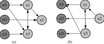
The DFS algorithm starts at the root node and then traverses the whole graph. Given the directed graph G, (example in Fig 2 (a)), if we need to measure ‘s sensitivity, the algorithm will start at exogenous factors (e.g., , and ) sequentially. Therefore, it traverses the graph three times in order to find whether there is a path from , and to node . Although it can measure the sensitivity in this way, it is not an efficient way when there is a large
Inputs: G, variable list, factor list
Procedure:
1: G’ = reverse arc’s direction of G
2: for each node n in variable list do
3: Stack S = {} // start with an empty stack 4: for each node u in G’, set u as unvisited 5: push S, n
6: while (S is not empty )do 7: u = pop S
8: if (u is not unvisited in G’), set u as visited 9: if (u is a node in factor list) then 10: increase sensitivity value of n 11: end if
12: for each unvisited neighbor w of u in G‘ do 13: push S, w
14: end for 15: end while 16: end for
17: max sensitivity = 0
18: for each node n in variable list do
19: if sensitivity value of n > max sensitivity then 20: max sensitivity = sensitivity value of n 21: clear sensitivity list and add n into the list 22: else if sensitivity value of n == max sensitivity 23: add n into sensitivity list
24: end if 25: end for
26: return sensitivity list
number of design variables and exogenous factors. In order to quickly find the sensitivity of a design variable, the directions of the arcs in the directed graph G are reversed in the proposed algorithm. The corresponding graph G’ is showed in Fig 2(b). In this case, the root nodes are now design variables. The DFS-based algorithm can then start at node and traverse the graph only once to find those paths from exogenous factors , and to node .
ef1 x1
ef2
ef3
x2
x3
ef1
ef2
ef3
x2 x1
x3
(a) (b)
Fig 2: (a) The directed graph G; (b) The reversed graph G’
[image:3.595.320.538.505.597.2]IV. CASE STUDY
In this section, a case study on the design of a hypothetical High Speed Rail (HSR) system is presented to illustrate how the sensitivity-based method can be used to effectively identify flexible design opportunities. The optimal flexible design opportunity is selected by comparing the sensitivity which is quantitatively measured by DFS-based algorithm. The optimal flexible design alternatives are analyzed and finally compared with traditional deterministic design.
A. Identify exogenous factors and design variables
[image:4.595.61.278.373.505.2]There are a number of characteristics that should be used in evaluating HSR systems. According to [14], these include travel demand, schedule performance, ride quality, noises, safety, energy conversion efficiency, actual travel time, reliability and so on. These factors are external to the HSR system, and they are the main sources of uncertainty to the HSR system. In this case study, five critical exogenous factors are selected. They are travel demand, ride quality, actual travel time, arrive on time rate, and energy conversion efficiency, as defined in Table 1. All of these exogenous factors are the sources of uncertainty because of the competition from air market and bus vehicle market, or technical innovation. The criteria of these exogenous factors are uncertain during the life cycle of HSR system.
Table 1: Exogenous factors in the hypothetical HSR system
Exogenous Factors Description
Travel demand
Predicted number of passengers in one year. It is growing as population expands in a particular region
Ride quality Comfortability of passenger‘s travel experience
Actual travel time The travel time for passenger between origin and destination
Arrive on time rate Ratio between the number of on time arrival train and total arrival train. Energy conversion
efficiency
System design efficiency with respect to energy consumption
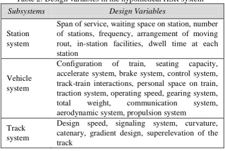
The HRS system is divided into three subsystems. They are station subsystem, vehicle subsystem and track subsystem. The design variables are identified according to [14]-[17], which are showed in Table 2.
Table 2: Design variables in the hypothetical HSR system
Subsystems Design Variables
Station system
Span of service, waiting space on station, number of stations, frequency, arrangement of moving rout, in-station facilities, dwell time at each station
Vehicle system
Configuration of train, seating capacity, accelerate system, brake system, control system, track-train interactions, personal space on train, traction system, operating speed, gearing system, total weight, communication system, aerodynamic system, propulsion system
Track system
Design speed, signaling system, curvature, catenary, gradient design, superelevation of the track
All of the relationships among exogenous factors and design variables are identified based on [14]. For example, the actual travel time is one of the exogenous factors. It is
affected by several variables. They are 1) train‘s ability to negotiate curves; 2) train‘s ability to accelerate and decelerate quickly; 3) number of station stops and dwell time at each station. Specifically, if passengers require shorter travel time, some variables within HRS system need to change, such as operating speed of the train, accelerate system, brake system, dwell time and number of station. The inter-relationships among design variables and exogenous factors in our hypothetical HRS system are represented using a direct graph, as showed in Fig 3.
B. Sensitivity evaluation
In this case study, there are 27 design variables and 5 exogenous factors. Using the proposed DFS-based algorithm, 12 design variables have sensitivity value 1, 14 design variables have sensitivity value 2, and 1 design variable has sensitivity value 3. It is found that the design variable of ―in-station facilities‖ is the most sensitive variable in this case. It is influenced by carrying capacity, ride quality and actual travel time directly and indirectly. Therefore, the HRS system will be more nimble in the future when the variable of in-station facilities is designed with flexibility. Next, we will add flexibility into the facilities and compare the flexible system design with deterministic design by the expected total cost.
C. Comparison
After indentifying the variables for embedding flexibility identified, the system designer needs to generate flexible design alternatives. Based on the analysis above, we analyze the ―in-station facilities‖ design variable. Specifically, we focus on pedestrian bridge‘s development in a station. Pedestrian bridge is built to transfer passengers to access the platforms. The number of bridges depends on travel demand in the region and ride quality of passengers. If fewer bridges are developed, the bridges may become too crowded when travel demand increases quickly. Even worse, it may exceed the capacity of the design. In such situation, these bridges require more maintenance cost, compared to regular maintenance cost. In addition, passengers‘ satisfaction may decrease. On the other hand, if more bridges are developed, extra annual maintenance cost is needed. Therefore, the problem here is to find how to design the pedestrian bridges in order to minimize total cost.
We assume that the deterministic forecast of travel demand in the first year is 7.5 million people, and rises exponentially in the future years. At the end of 30 years, the travel demand will increase to 12.41 million. In the real world, the actual travel demand is uncertain, given the long time horizon. We assume that the uncertainty of future demand is 50%, and the annual volatility for growth is 15%. The designed flow rate of the pedestrian bridge is 5000 people per hour. The peak hour demand is 2.5 times the regular demand. The assumed construction cost and maintenance cost are shown in Table 4. The number shows in Table 4 is relative cost. The extra maintenance cost is required when the actual travel demand exceeds the designed flow rate. The decreased satisfaction from passengers is also represented by cost, which is called satisfaction reduction cost.
[image:4.595.60.282.581.729.2]Superelevation of
the track Propulsion system
Seating capacity per car
Gradient design Personal space on
train Frequency
of the train Span of service time
Design speed of the track
Number of stations Dwell time at
each station
Track-train interactions Waiting space on
station
Catenary
Brake system
Total weight
Traction system
Curvature
Gearing system
Communication system Control system
Arrangement of moving rout
In-stations facilities
Signaling system
Accelerate system Configuration of
the train
Operating speed of the train
Aerodynamic system
Travel demand Ride quality Actual traveltime Arrive on timerate Energy conversionefficiency
Station subsystem
Vehicle subsystem
Track subsystem Exogenous factors
[image:5.595.91.512.51.205.2][image:5.595.80.257.252.355.2]
Fig 3: The constructed directed graph of the hypothetical HSR system
Table 4: Construction and maintenance cost per year (×1000)
Category Cost
Initial construction cost per bridge 5000
Maintenance cost for year 1-5 20
Maintenance cost for year 6-20 100
Maintenance cost for year 21-30 200
Extra maintenance cost per person 2
Satisfaction reduction cost per person 1
Based on the above information, three design alternatives are compared in this section:
1) Deterministic design A Build one pedestrian bridge in station.
2) Deterministic design B Build two pedestrian bridges in station
3) Flexible design C Build first pedestrian bridge in station. Meanwhile, design the footings and columns for the second bridge. When the actual travel demand exceeds the designed flow rate of the bridge in two consecutive years, the second bridge will be built. The initial cost for flexible design is 8 million and the construction cost for the second bridge is 4 million. Compared to the deterministic designs, the initial cost for flexible design is increased. However, this is the premium to acquire the real option for future easy update.
The total cost of design alternatives A or B is calculated as follows:
(1)
is the total cost of design A or B, is the initial
cost for construct the bridge, , , and are the annual
maintenance cost, extra maintenance cost and satisfaction reduction cost at each year i respectively. When the actual travel demand for peak hour exceeds the designed flow rate at year i, and are needed. Otherwise, both of these two
terms are zero in equation (1). The equation for calculating the total cost of flexible design C is different from equation (1), which shows as follows:
(2)
where , are the initial cost and the maintenance cost
for building second bridge respectively, and the meanings of
,and are the same as equation (1). When the
actual travel demand for peak hour exceeds the designed flow rate of the bridge in two consecutive years, the second bridge will be built. Therefore, and are calculated in
equation (2). Otherwise, and are zero in equation
(2). It should be noted that the discount rate for calculating the total cost is assumed to be 12%.
(a)
(b)
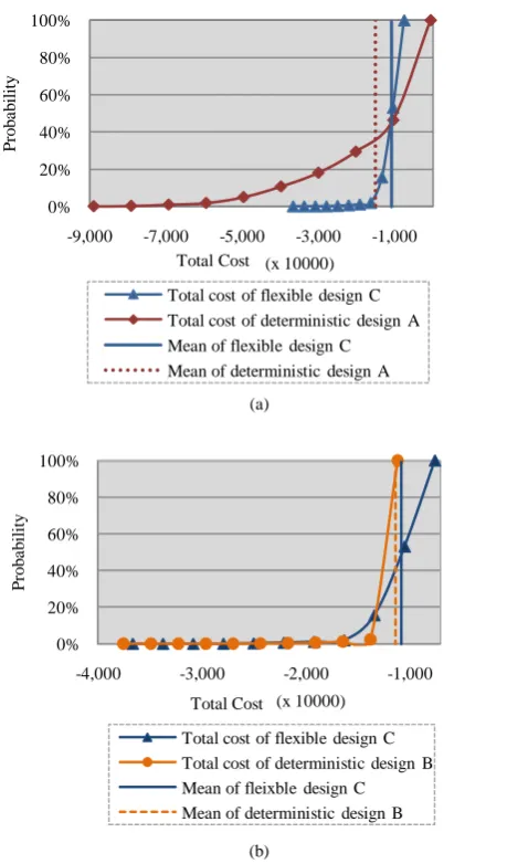
Fig 4: (a) Cumulative distribution of design A and design C (b) Cumulative distribution of design B and design C
0% 20% 40% 60% 80% 100%
-9,000 -7,000 -5,000 -3,000 -1,000
P
ro
b
a
b
il
it
y
Total Cost (x 10000)
Total cost of flexible design C Total cost of deterministic design A Mean of flexible design C Mean of deterministic design A
0% 20% 40% 60% 80% 100%
-4,000 -3,000 -2,000 -1,000
P
ro
b
a
b
il
it
y
Total Cost (x 10000)
[image:5.595.311.541.358.749.2]Monte Carlo Simulation is used to generate 3000 sets of random travel demand for this case. The corresponding total cost is calculated according to equation (1) and (2). The cumulative distributions of total cost for the three design alternatives are compared in Fig 4 (a) and (b). It should be noted that cost is outflow from the perspective of system design. So negative value is used to represent cost in Fig 4 (a) and (b). Fig 4 (a) presents the cumulative distribution of deterministic design A and flexible design C. It shows that adding flexibility in pedestrian bridge design greatly decreases both maximum total cost (from 98.86 million to 36.63 million) and the expected total cost (from 15.13 million to 10.80 million). Fig 4 (b) compares the cumulative distribution of deterministic design B and flexible design C. It shows that the expected total cost of flexible design is less than deterministic design B (10.80 million vs. 11.35 million). In addition, the maximum total cost is slightly less than deterministic design B (36.63 million vs. 37.54 million).
V. CONCLUSION
In this paper, a sensitivity-based method is proposed to identify where the flexibility should be added in a system. The design variable is sensitive in the neighborhood of an exogenous factor when the exogenous factor directly or indirectly affects design variable . Specifically, the changes of exogenous factor can instigate the changes of design variable . The design variable, influenced by more exogenous factors, is more sensitive, compared to other design variables. The most sensitivity design variables are the potential flexible design opportunities which are selected by DFS-based algorithm, and finally add flexibility in the later design process. A hypothetical HSR system is designed to illustrate how to use sensitivity-based method to identify potential flexible design opportunities. The case study shows that the flexible design strategy can greatly decrease both the maximum total cost and expected total cost, compared with deterministic design strategy.
The proposed approach has the following advantages. Firstly, the proposed approach is more suitable for the system which has a large number of design variables and complex relationships. It is difficult to identify all the relationships among exogenous factors to design variables within these systems. The sensitivity-based method not only considers the direct relationships but also considers the indirect relationships. Therefore, the possible source of uncertainty for particular design variable can be fully investigated. Secondly, the sensitivity of design variable is clearly defined in this paper. The sensitivity of each variable can be quantitatively measured by counting the number of affecting exogenous factors, which can instigate the changes of a particular design variable. Thirdly, the DFS-based algorithm is proposed to quickly measure the sensitivity of each design variable. The potential flexible design opportunities are the design variables, which are selected by the DFS-based algorithm.
A future investigation might focus on the selection of potential flexible design opportunities. In this paper, we only consider the design variables and their sensitivities for evaluating the flexible design opportunities. However, other factors may also affect the result in real practice, such as the
probability that exogenous factor may change in future and the switch cost of changing design variables. All these factors need to be incorporated in future work.
REFERENCES
[1] J. H. Saleh, G. Mark and N. C. Jordan, ―Flexibility: a multi-disciplinary literature review and a research agenda for designing flexible systems,‖ Journal of Engineering Design, vol. 20, no. 3, 2008.
[2] T. Wang, ―Real options ‗in‘ projects and systems design—identification of options and solutions for path dependency,‖ Ph.D. dissertation, engineering systems division, MIT, 2005.
[3] K. Kalligeros, O. de Weck, R. de Neufville and A. Luckins, ―Platform identification using design structure matrices,‖ Sixteenth Annual International Symposium of the International Council On Systems Engineering (INCOSE), Orlando, Florida. 2006.
[4] J. Lin, ―Exploring flexible strategies in engineering systems using screening models –applications to offshore petroleum projects‖ Ph.D. dissertation, engineering systems division, MIT, 2008.
[5] A. N. Ajah and P. M. Herder, ―Addressing Flexibility during Process and Infrastructure Systems Conceptual Design: Real Options Perspective,‖ IEEE International Conference on Systems, Man and Cybernetics, 10-12 Oct., Vol. 4, pp. 3711-3716. 2005.
[6] T. Zhao and C. L. Tseng, ―Valuing Flexibility in Infrastructure Expansion,‖ Journal of Infrastructure Systems, Vol. 9, No. 3, pp. 89-97.2003.
[7] M. A. Cardin and R. de Neufville, ―A survey of state-of-the-art methodologies and a framework for identifying and valuing flexible design opportunities in engineering systems,‖ working paper, 2008. Available:
http://ardent.mit.edu/real_options/Common_course_materials/papers. html
[8] R. de Neufville, S. Scholtes, and T. Wang, ―Valuing Options by Spreadsheet: Parking Garage Case Example,‖ ASCE Journal of Infrastructure Systems, Vol. 12, No.2. pp. 107-11.2006.
[9] E. S. Suh, O. L. de Weck and D. Chang, ―Flexible Product Platforms: Framework and Case Study‖, Research in Engineering Design, Vol.18, No. 2, pp. 67-89. 2007.
[10]K. Kalligeros, ―Platforms and real option in large-scale engineering systems,‖ Ph.D. dissertation, Engineering Systems Division, MIT, 2006.
[11] J. E. Bartolomei, ―Qualitative knowledge construction for engineering systems: extending the design structure matrix methodology in scope and procedure,‖ Ph.D. dissertation, engineering systems division, MIT, 2007.
[12] M. A. Cardin, ―Facing reality: design and management of flexible engineering systems,‖ Master of Science Thesis, Technology and policy, MIT, 2007.
[13] T. H. Cormen, C. E. Leiserson, R. L. Rivest and C. Stein, ―Introduction to algorithms,‖ Cambridge, Mass. MIT Press, 2009.
[14] R. K. Whitford, M. Karlaftis and K. Kepaptsoglou, ―High-speed ground transportation: planning and design issues,‖ 2003. Available: http://freeit.free.fr/The%20Civil%20Engineering%20Handbook,2003/ 0958%20ch60.pdf
[15] J. S. Chou and C. Kim, ―A structural equation analysis of the QSL relationship with passenger riding experience on high speed rail: an empirical study of Taiwan and Korea,‖ Expert System with Applications, vol. 36, pp.6945-6955, 2009.
[16] J. Campos and G. de Rus, ―Some stylized facts about high-speed rail: a review of HSR experiences around the world,‖ Transport Policy, vol. 16, pp. 19-28, 2009.