Abstract— In this work, we resolve the problem of robustly stabilizing nonlinear feedback systems in the presence of disturbance signals (noise) at each subsystem. The process of stabilizing the system is achieved using Integrator backstepping that incorporates saturation functions as part of the controls. The resulting controller is tested to see its effectiveness under noise bombardment. The systems response upon application of the controller is one whose trajectory is globally stable, in order words, we have developed and implemented robust controller that can stabilize systems with uncertainties and noise at each subsystem.
Index Terms—Integrator backstepping, noise, robust controller, saturation function, stabilization, trajectory
I. INTRODUCTION
HE problem of of stability and stabilization of control systems has been the subject of much research over the years. These research efforts have produced such very powerful techniques like stability in the sense of Lyapunov, and its various extensions and converses, see Lyapunov [16], Massera [18], LaSalle [12], and Kurzweil [11]. Also, the problem of generating Lyapunov functions has been addressed and is still been addressed by a number of notable researchers, including Krasovskii [9], Lin [14], Lin and Sontag [15].
Quite recently, the concept of Integrator backstepping was introduced as a recursive control design tool. The earliest record of application of this control design methodology can be seen implicitly in the works of Parks [20], Tsinias [22], Kodistchek [8], Brynes and Isidori [2], Sontag and Sussmann [21]. However, a formal presentation on the design of adaptive control laws was seen in the works of Kanellakopolous, et al [6], while authoritative expositions on the subject can be found in Krstic et al [10], Marino and Tomei [17], Isidori [3, 4], Khalil [7], and Tsinias [23]. The process has been successfully used to design a wide range of control systems like Non Holonomic systems, adaptive control systems, Tracking Controllers, real life problem definitions in areas of Electric Machines, Steering and
John. A. Akpobi is a Professor in the Department of Production Engineering, University of Benin, Benin City, Nigeria. ( Corresponding author’s phone number: +2348055040348; e-mail: alwaysjohnie@ yahoo.com).
G. C. Ovuworie is a Professor in the Department of Production Engineering, University of Benin, Benin City, Nigeria.
Braking Control, tracking control of nonlinear mechanical systems [13], nonlinear control of underactuated mechanical systems with application to robotics and aerospace vehicles [19], etc.
In Tsinias [23], the problem of Backstepping Design for Time-Varying Nonlinear Systems with Unknown Parameters, was considered. However, the unknown was allowed to be within a class of measurable bounded maps. Thus, uncertainty in terms of noise and unboundedness, was not considered.
The problem of robustifying control laws against unmodeled dynamics has been a well-studied and fruitful area of research. Arcak, et al [1] proposed two redesign methods to robustify backstepping control laws against dynamic uncertainties at the input of the plant. These are the passivation and truncated passivation techniques. The cancellation and LGV - backstepping approaches investigated
in [1] is suitable for the nominal system. However it does not guarantee global asymptotic stability (GAS) in the presence of unmodeled dynamics. They imposed a limitation on the unmodeled dynamics, in that it was required to be minimum phase and relative degree zero. Consequently their method cannot be used to stabilize systems that are not minimum phase and not relative degree zero. Also, they do not address the problem of disturbance (noise signals) in other parts of the system apart from the input stage.
For control systems in which the input dynamics are ignored, Jiang and Arcak [5] used the method of input to state stability (ISS), coupled with small gain theorem to achieve global asymptotic stability (GAS). The essence of this study was to remove the stability restriction on the ignored input dynamics in earlier works. Their resulting control law guaranteed boundedness of closed-loop solutions, and their convergence to a compact set around the origin which can be rendered arbitrarily small. They ignored some of the subsystems since it destroyed the feedback structure of the overall system and restricted the other part to be minimum phase and relative degree zero. Again they did not address the problem of disturbance (noise signals) in other parts of the system .
In this work, we extend backstepping to achieve robust stabilization of nonlinear systems in the presence of disturbance (noise) signals at each subsystem using saturation functions. The process involves saturating the noise first and then recursively stabilizing the subsystems by applying integrator backstepping technique. The controllers
A Generalized Robust Stabilization of
Nonlinear Feedback Systems in the Presence of
Disturbance (Noise) Signals at each Subsystem,
using Integrator Backstepping with Saturation
Functions
John A. Akpobi, Member, IAENG and G. C. Ovuworie
T
designed using this method are not restricted to systems that are minimum phase and relative degree zero.
II. DEFINITIONS
In this section we give the following definitions needed in the development of the results:
A. Lyapunov Function
A Lyapunov function is defined as follows:
Let be a
C
1 function defined in a domain that includes the origin. Then the Lyapunov function,V (t, x ), which must satisfy the following conditions:1. V is proper at the equilibrium state
x
e;
n
x
R V x
(1) that is, V is a compact subset of some neighborhood O of
e
x
for each 0 small enough.2. V is positive definite on O:
e0
V x
and 0,
x
x
e (2)For
x
x
e in O there is some timet
1
T
,t
1 0 and some controlu U
[0, )t1 admissible for x such that the trajectory
x u
,
resulting from the control and this initial state,V
t
V x
t
0,
t
1
and
1
V
t
V x
.3 as
(3) This third property is referred to as radially unbounded or uniformly unbounded or weakly coercive.
B. Saturation Function
We define a saturation function
i,
as follows: (4) where
iis the saturation level
sgn
is the signum function defined as:
1
0
sgn
0
0
1
0
if
if
if
(5)
III. MAINRESULTS
In this section we present the main results of this work in the theorem of subsection 3.1 with proofs. Then we provide a systematic algorithm for obtaining the stabilizing controller using the method of Integrator backstepping with saturation function to eliminate the noise.
A.Theorem
Given a feedback control system with disturbance signal at each subsystem of the form:
, ,
, ,
n m n
x
f x u
x
R
u
R
R
(6) Then, the existence of a controller of the form:
,
,
, where
u
k x
is a saturation function such thatdV
0 or
dV
x
2dt
dt
is a necessary andsufficient condition for the resulting closed loop control system to be robustly globally (locally) asymptotically stable.
B. Proof
Necessity:
We need to show that the existence of the control
,
,
u
k x
is a necessary condition for robust global (local) asymptotic stability of the system.Assume that the controller
u
k x
,
,
exists and transformsf x u
, ,
, tof x
,
,
0
. Using Lyapunov’s stability condition, select a functionV x
that isC
1. For global (local) asymptotic stability, we have;
20, or
dV x
dV x
x
dt
dt
. Evaluating this wehave:
dV x
dV x
dx
dt
dx
dt
this yields
, ,
dV x
f x u
dx
. (7) The disturbance
is unknown and has the tendency to makef x u
, ,
0
and consequently
, ,
0
dV x
f x u
dx
, hence instability is obtained. Since we have no information about this disturbance, we cannot select the control u to incorporate the negative of the noise. Thus it is not realizable to cancel the effect of the noise. Hence, there is the need to saturate it (using the saturation function
,
) to a finite gain that can easily be resolved. Consequently, we can obtain the controller that no longer incorporates the destabilizing noise but the:
nV R
R
R
n
D
R
V x
x
O
,
V x t
x
,
sgn
min
,
i i i i i i
saturated signals. Thus, we have
u
k x
,
,
. Now since the controlu
k x
,
,
makes
, ,
0
f x u
that isf x k x
,
,
,
0
, and V(x) is positive definite, proper and radially unbounded,0
dV
dx
dV
dV dx
dt
dx dt
dV
f x k x
,
,
,
0.
dx
(8)= (positive).(negative)=negative If
dV
0,
x
R
ndt
then we have robust globalasymptotic stability (controllability if the control
u
0
) while it is said to be robust local asymptotic stability (controllability if the controlu
0
) if0,
ndV
x
D
R
dt
Next we prove sufficiency condition. Sufficiency :
Since the system is robustly globally (locally) asymptotically stable, using Lyapunov stability condition we have that:
( )
dV x
dt
=
2
0, or
dV x
dx
x
dx
dt
=
dV
f x u
( , , )
0 or -
x
2
dx
(9)from which
u
k x
( , )
Now
, is a disturbance which we have no information about. So, we cannot use cancellation technique to eliminate it from the system. Hence, the instability remains. Since the controller would still be unable to cancel the destabilizing effect of the noise, consequently we have to saturate the noise or disturbance
to a finite level
that we can control. The incorporation of the saturation function transforms the noise to the form:
,
. This transforms the control to the form:u
k x
,
,
. Thus robust global (local) asymptotic stability is a sufficient condition for the existence of controller of the form
,
,
u
k x
.C. Development of Integrator Backstepping Based Controller
Consider a feedback control system described by:
(10)
where the above system is
C
with and . This system is assumed to be locally Lipschitzi.e.
x y
,
R
n
0,
t
t
. (11)The above system has a lower triangular structure, as shown in (12).
Thus, in strict feedback form we have the control system as:
1
:
2
:
x
2
f
2
x x x
1,
2,
3,
2
3
:
x
3
f
3
x x x x
1,
2,
3,
4,
3
1
:
n
x
n1
f
n1
x x x x
1,
2,
3,
4,....,
x
n,
n1
:
n
1,
2,
3,
4,....,
, ,
n n
n n
x x x x
x
f
x u
(12)Procedure:
First we saturate the noise signals through saturators
i
as follows:(13) where
iis the saturation levelEquation (13) follows the standard definition of a saturation function.
So the system now becomes:
1 1 1 2 1 1 1 1
:
x
f x x
,
,
,
2 2 1 2 3 2 2 2 2
:
x
f
x x x
,
,
,
,
3 3 1 2 3 4 3 3 3 3
:
x
f
x x x x
,
,
,
,
,
1 2 3 4 1 1
1
1 1 1
,
,
,
,..,
:
,
,
n n
n
n n n n
x x x x
x
f
x
1
,
2,
3,
4,..,
:
, ,
,
n n
n
n n n n
x x x x
x
f
x u
(14)Treat as input, and define it as
x
2
x
1,
1,
1
such that subsystem 1 is exponentially stable. So, we have: (15) to be exponentially stable. Forexample,
,
x
f x u
n
x
R
mu
R
,
,
f t x
f t y
L x
y
1 1 1
,
2,
1x
f
x x
i
,
sgn
min
,
i i i i i i
2
x
1 1 1
,
1,
1 1x
f x
x
(16) and select the Lyapunov function
12 12
x
V x
(17)
1
1 1 1 1 1 1
,
,
x
V
x
f
x
x
t
(18)To track and back step the integrator, we define:
2 2 1 1
,
1 1,
1z
x
x
(19) This gives:
2 2 1 1
,
1 1,
1z
x
x
(20) Then, consider the subsystem:
1 1 1 2 1 1 1 1 1 1
:
x
f x z
,
x
,
,
2 2 1 1 1 1 1 2
:
z
x
x
,
,
(21)But
x
2
f
2
x x x
1,
2,
3,
2
2,
2
, therefore
1 1 1 2 1 1 1 1 1 1
:
x
f x z
,
x
,
,
2 2 1 2 3 2 2 2 2
1 1 1 1 1
:
,
,
,
,
,
,
z
f
x x x
x
(22)But from (9)
x
2
z
2
1
x
1,
1
1,
1
, therefore we have:
1 1 1 2 1 1 1 1 1 1
:
x
f x z
,
x
,
,
1 22 2 1 1 1 1 1 2
3 2 2 2 1 1 1 1 1
,
:
,
,
,
,
,
,
,
x z
z
f
x
x
x
(23)Select the Lyapunov function as:
2 2 1 2 2
2
2
x
z
V
(24) This gives:
2 22 1 2 1 2 1 2
,
V
V
V
x z
x
z
x
z
x
1.
f x z
1
1,
2
1
x
1,
1
1,
1
1 2 1 1 1 1 1 2 2
3 2 2 2 1 1 1 1 1
,
,
,
,
,
,
,
,
x z
x
z
f
x
x
(25)Solve for such that
V
2
x z
1,
2
0
to achieve stability. Input the value of into subsystem 2.But
x
3 is not the control, so, define a new variable:
1 2 1 1 1 3 3 3
2 2 2
,
,
,
,
,
x z
z
x
(26)To backstep, we differentiate as follows:
3 3
3 1 2 1 1 1 2 2 2
,
,
,
,
,
z
x
x z
(27)We proceed in the same manner as above until we get to the last step. Define the new state variable as
1 2 1 1 1 1 1
2 2 2
,
,..,
,
,
,
,
,..,
,
nn n n
n n n
x z
z
z
x
(28)To backstep, differentiate
1 2 1 1 1 1 1
2 2 2
,
,..,
,
,
,
,
,..,
,
nn n n
n n n
x z
z
z
x
(29)Substitute for
x
nfrom the original system. Then, substitute forx x
2,
3,...
x
nin the resulting subsystem. With u as the input, use a Lyapunov functionand solve for stability and obtain a value for u that is
1 2 3 1
1 2 31 2 3
1 1
,
,
,...
,
...
0
cn cn cn
cn n n
cn cn
n n
n n
V
V
V
V
x x x
x
z
x
x
x
x
x
x
V
V
x
z
x
z
= < 0 (30)
IV. ILLUSTRATIVEEXAMPLES A. Example 1
Consider the system:
1
:
x
1
x
12
x
2
1
t
2
:
x
2
x
13
x
2
x
3
2
t
3
:
x
3
2
x
1
x
2x
3u
3
t
(31)In the above system,
i( )
t i
1, 2, 3
represents the noise (disturbance) signal.For an input u=sin(t) and a band limited white noise as shown in Figure 1
in stabilizing the system we proceed as follows:
1 1
x
x
2
x
3x
3x
)
,
,...,
,
(
1 2 n1 n1cn
x
x
x
z
Saturate the noise signals
1
t
,
2
t
,
3
t
as
1 1
,
,
2
2,
,
3
3,
, thus we have:
1 1 2 1 1 1
:
x
x
2
x
,
2 1 2 3 2 2 2
:
x
x
3
x
x
,
3 1 2 3
3 3 3
:
2
,
x
x
x
x
u
(32)For the subsystem
1
,
let us treatx
2 as the virtual control or input and select its value such that we have stability. Let
1
2 2 1
,
1 1 1x
x
x
(33) Therefore
1 1
2
1 1 1x
x
x
1
x
x
(34) Using the Lyapunov function,
122
x
V x
(35) we have
11 1
1
V x
V x
x
x
x
12 (36) and
x
120
hence the subsystem1
,
is asymptotically stable. Butx
2 is not the control so we introduce a variable2
z
to track error and then carry out integrator backstepping. Set
2 2 1 1
,
1z
x
x
(37) which gives
2 2 1 1
,
1z
x
x
1 2 2 2 1 1
z
x
x
(38) But from subsystem1
and2
,
1 1
2
2 1 1,
x
x
x
2 1
3
2 3 2 2,
x
x
x
x
Therefore,
2 1 2 3 1 1 2 2 1 1
3
1.5
,
,
0.5
,
z
x
z
x
(39)This implies that
1 1 2 1
:
x
x
2
z
2 1 2 3 1 1 2
2 2 1 1
:
3
1.5
,
,
0.5
,
z
x
z
x
(40) Define
12 222 1
,
22
2
x
z
V
x z
(41)Hence,
1 2 3
1 1 2 2 1 1 2 2 1 1
3
2
1.5
,
,
0.5
,
x
z
x
V
x
x
z
z
2 21 2 1 2 2 3 2 1 1
2 2 2 2 1 1
5
1.5
,
,
0.5
,
x
z x
z
z x
z
z
z
(42)For
V
x
12z
22,
3 1 1 1 2 2 1 1
5
1.5
,
,
0.5
,
x
x
(43)This gives
z
2
2
x
1
z
2 (44)Define
3 3 2 1
,
2,
1 1,
,
2 2,
z
x
x z
(45) with
2 1 2 1 1 2 2 1 2 1 1 2 2 1 1
,
,
,
,
,
5
1.5
,
,
0.5
,
x z
x
z
(46) Therefore,
3 3 1 2 1 1 2 2 1 1
5
1.5
,
,
0.5
,
z
x
x
z
(47)and
3 3 1 2 1 1 2 2 1 1
5
1.5
,
,
0.5
,
z
x
x
z
(48)
Replacing
x
1,z
2andx
3with their values gives
3 1 2 3 1 1 2 2 1 1
2 2 1 1
7
12
1.5
,
,
0.5
,
,
0.5
,
z
x
z
z
u
(49) Define
12 22 323 1
,
2,
32
2
2
z
x
z
V x z z
(50) Therefore,
1 2 3 2 2
3 1 2 3 1 2 3
1 1 2 2 1 1 2 2 1 1
7
12
,
,
1.5
,
,
0.5
,
,
0.5
,
x
z
z
V x z z
x
z
z
u
(51)
2 2
3 1 2 3 1 2 3 1 2 2 3 3 3
3 1 1 2 3 1 3 1 1 3 2 2 3 1 1
,
,
7
12
1.5
,
,
0.5
,
,
0.5
,
V x z z
x
z
z
x
z z
z
uz
z
z
z
z
z
(52) For
V x z z
3
1,
2,
3
x
12z
22z
32
1 2 3 1 1 2 2 1 1 2 2 1 1
7
12
2
1.5
,
,
0.5
,
,
0.5
,
u
x
z
z
(53)
Substituting for
u
inz
3gives:3 3
z
z
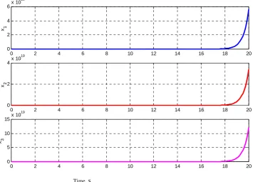
(54)Therefore we simulate the resulting system (eqn.55), considering three different initial conditions:
case1:
x
1
0
5
z
2
0
9
z
3
0
7
case2:
x
1
0
0.002
z
2
0
0.008
z
3
0.005
case3:
x
1
0
8000
z
2
0
5000
z
3
0
9000
The simulation results are shown in Fig. 1.
[image:6.595.42.558.44.511.2]Time (s)
Fig. 1. System input(control, U=Sin(t) and d(t)= Band Limited white noise
The response of the system is shown in Fig. 2
0 2 4 6 8 10 12 14 16 18 20 -1
-0.5 0 0.5 1
u=
s
in
(t
)
0 2 4 6 8 10 12 14 16 18 20 -4
-2 0 2 4
d(t
)=
B
a
nd
lim
it
ed
w
h
it
e
no
is
[image:6.595.144.454.184.500.2]Time s
Fig. 2. System response to inputs
[image:7.595.110.482.335.600.2]Fig. 3. State Trajectories of the stabilized system for case 1
0 2 4 6 8 10 12 14 16 18 20
0 2 4 6x 10
19
x1
0 2 4 6 8 10 12 14 16 18 20
0 2 4x 10
19
x2
0 2 4 6 8 10 12 14 16 18 20
0 5 10 15x 10
19
x3
0 2 4 6 8 10 12 14 16 18 20
-10 -5 0 5
x1
0 2 4 6 8 10 12 14 16 18 20
-20 -10 0 10
z2
0 2 4 6 8 10 12 14 16 18 20
-10 -5 0
Time (s)
z3
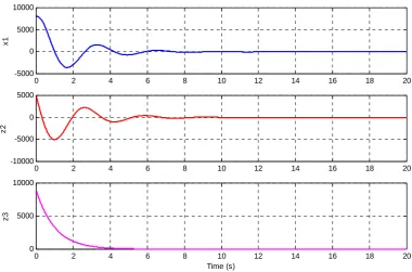
Fig. 4. State Trajectories of the stabilized system for case 2
Fig. 5. State Trajectories of the stabilized system for case 3
B. Example 2
Consider the following pendulum equation in state space form with friction and noise:
1 2 1
x
x
t
2
10sin
1 2 2x
x
x
u
t
(56)This example is a modified benchmark problem which can be found in standard control texts and journal papers [7, 23].
When there is no noise signal, and
u
0
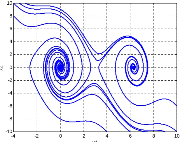
, the phase portrait shows that the equilibrium point (0,0) is a stable focus and while the other equilibrium point
, 0
is a saddle point. This is shown in Figure 6.0 2 4 6 8 10 12 14 16 18 20
-10 -5 0 5x 10
-3
x1
0 2 4 6 8 10 12 14 16 18 20
-10 -5 0 5x 10
-3
z2
0 2 4 6 8 10 12 14 16 18 20
-6 -4 -2
0x 10
-3
Time (s)
z3
0 2 4 6 8 10 12 14 16 18 20
-5000 0 5000 10000
x1
0 2 4 6 8 10 12 14 16 18 20
-10000 -5000 0 5000
z2
0 2 4 6 8 10 12 14 16 18 20
0 5000 10000
Time (s)
[image:8.595.104.485.357.608.2]Fig. 6. Phase Portrait of the Pendulum showing stable focus and saddle point
[image:9.595.123.471.352.585.2]With the presence of noise (
1
t
and
2
t
) in form of wind, the system, behaves in an unstable manner as shown in Figure 7.Fig. 7. The unstable response of the Pendulum system with noise and friction
To stabilize the system
Using this method, after some computations for stage 1, the virtual control x2 is selected as
2
2
1 1 1,
x
x
t
(57) with Lyapunov function:
12 12
x
V x
(58)The Lyapunov function for stage 2 is:
2 2 1 2 2
2
2
x
z
V
x
and the controller designed using this method is given as:
1 1 2 2 2 1 1 1 1
10 sin
2
,
,
,
u
x
x
z
t
t
t
(59)Applying these controls, the resulting system is given as:
1 1 2
x
x
z
2 1 2
z
x
z
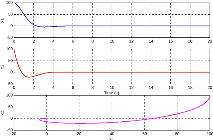
(60) This system is then simulated and the response shown in Fig, 8.-4 -2 0 2 4 6 8 10
-10 -8 -6 -4 -2 0 2 4 6 8 10
x2
x1
50 55 60 65 70 75 80 85 90 95 100
-40 -20 0 20
x1
50 55 60 65 70 75 80 85 90 95 100
-10 0 10
Time (s)
x2
-35 -30 -25 -20 -15 -10 -5 0 5 10
-10 0 10
x2
Fig. 8. Trajectory of the stabilized Pendulum
V. DISCUSSIONOFRESULTS
[image:10.595.109.482.66.310.2]Two (Examples1 and 2) systems were simulated on a computer using SIMULINK™ software of MATLAB™. The responses are shown in Figs. 1-5, for the first system, while Figs. 6-8 shows the response of the second system. In Fig.1, the systems control (input) signals in this case a sinusoidal wave and disturbance (White noise with Limited bandwidth) are outputted.
The time response of the states of the original system, for Example1, is shown in Fig. 2. This is a highly unstable motion. The deviations from the equilibrium position are so large, in the order of 103 in 18 seconds for all the states. This is due to the presence of disturbance (noise). In Figs. 3-5, the system’s response under the designed stabilizing controller shows a stabilized trajectory that converges fast (about 8 seconds) to the equilibrium.
For the second system considered, the phase portrait of the undisturbed system is shown in Fig. 6, in which the system for the equilibrium points (0, 0) and
, 0
behaves as a stable focus and a saddle point respectively. However, the inclusion of noise bombardment in form of wind, causes the system to produce a highly unstable trajectory as shown in Fig. 7. Upon application of the controller designed using our method, the system’s motion is a stabilized trajectory as shown in Fig. 8. The system converges (within 4 seconds) to the equilibrium.VI. CONCLUSION
A recursive technique based on Integrator backstepping coupled with saturation functions has been developed and implemented for robust stabilization of nonlinear feedback systems. The systems considered were subjected to disturbance (noise) signals at each subsystem
The noise in the systems used as benchmark examples, was effectively controlled using saturation functions, with an appropriate saturation level. The use of saturators effectively dampens and to a great extent eliminates the effect of the noise so as to achieve stability.
The computer simulation of the resulting systems (the implementation of the developed controller on the original systems), showed stabilized trajectory of the system’s states that were previously noisy and unstable. The trajectory of the stabilized systems shows fast response in approaching equilibrium. Thus it is clear that stabilization was achieved when the developed controllers were implemented on the systems considered.
APPENDIX:NOMENCLATURE
,
t T
Timeu
control variable
V
Lyapunov functionx
state variables
saturation function
saturation level
noise or disturbance signal
TrajectoryREFERENCES
.
[1] M. Arcak, M. Seron, J. Braslavsky, and P. Kokotovic, “Robustification of Backstepping against Input Unmodeled Dynamics”, IEEE Transactions on Automatic Control, Vol. 45, No 8, 2000. pp. 1358-1363.
[2] C. I. Byrnes, and A. Isidori, “New Results and Examples in Nonlinear Feedback Stabilization”, System and Control Letters, Vol. 12, 1989, pp. 437-442.
[3] A. Isidori, Nonlinear Control Systems, 3rd Edition (4th Printing, 2002)
Springer- Verlag, Berlin, 1995.
0 2 4 6 8 10 12 14 16 18 20
-50 0 50 100
x1
0 2 4 6 8 10 12 14 16 18 20
-50 0 50 100
Time (s)
x2
-20 0 20 40 60 80 100
-50 0 50 100
x2
[4] A. Isidori, Nonlinear Control Systems II, Springer- Verlag, London, 1999.
[5] Z.P. Jiang, and M. Arcak, “Robust Global Stabilization with Ignored Input Dynamics: An ISS Small-gain Approach”, IEEE Transactions
on Automatic Control, Vol. 46, No. 9, 2001, pp. 1411-1415.
[6] I. Kanellakopoulos, P. V. Kokotovic, and A. S. Morse, “Systematic Design of Adaptive Controllers for Feedback Linearizable Systems”,
IEEE Transactions on Automatic Control, Vol. 36, No 11., 1991,
pp.1241-1253.
[7] H. K. Khalil, Nonlinear Systems, 3rd Edition, Prentice Hall, Upper Saddle River, New Jersey, 2002.
[8] D. E. Koditschek, “Adaptive Techniques for Mechanical Systems”,
Proceedings of the 5th Workshop on Adaptive Systems, New Haven,
CT, 1987, pp. 259-265.
[9] N. N. Krasovskii, Stability of Motion: Applications of Lyapunov’s
Second Method to Differential Systems and Equations with Delay,
Stanford University Press, Stanford, California, 1963.
[10] M. Krstic, I. Kanellakopolous, and P. Kokotovic, Nonlinear and
Adaptive Control Design, Wiley-Interscience, New York, 1995.
[11] J. Kurzweil, “On the inversion of Lyapunov’s Second theorem of Stability of Motion” Translations of American Mathematical Society, ser.2, Vol. 24, 1956, pp. 19-77.
[12] J. P. LaSalle, “An Invariance Principle in the Theory of Stability”, in Hale, J.K. and LaSalle, J.P., (editors), Differential Equations and
Dynamical Systems, 1967, pp. 277-286, Academic Press, New York.
[13] A. A. J. Lefeber, “Tracking Control of Nonlinear Mechanical Systems”, PhD Thesis, Universiteit of Twente, 2000.
[14] Y. Lin, “Lyapunov Function Techniques for Stabilization”, PhD Dissertation, Rutgers University, New Brunswick, NJ, 1992.
[15] Y. Lin, and E. D. Sontag, “Control-Lyapunov Universal Formulae for Restricted Inputs”, Control: Theory and Advanced Technology, Vol. 10, 1995, pp. 1981-2004.
[16] A. M. Lyapunov, “The General Problem of Motion Stability”, in Russian, 1892, Translated In French. Ann Fac Sci. Toulouse, Vol. 9 1907, pp. 203-474. Reprinted in Ann. Math. Study, No 17, Princeton University Press, 1949.
[17] R. Marino and P. Tomei, Nonlinear Control Design: Geometric,
Adaptive, Robust, Prentice-Hall, New York, 1995.
[18] J. L. Massera, “Contribution to Stability Theory”, Annals of
Mathematics, Vol. 64, 1956, pp. 182-206.
[19] R. Olfati-Saber, Nonlinear Control of Underactuated Mechanical
Systems with Application to Robotics and Aerospace Vehicles, PhD
Thesis, Massachusetts Institute of Technology, 2001.
[20] P. C. Parks, “Lyapunov Redesign of Model Reference Adaptive Control Systems”, IEEE Transactions on Automatic Control, Vol. 11, 1966, pp. 362-367.
[21] E. D. Sontag and H. J. Sussmann, “Further Comments on the Stabilizability of the Angular Velocity of a Rigid Body”, Systems and
Control Letters, Vol. 12, 1988, pp. 437-442.
[22] J. Tsinias, “Sufficient Lyapunov-Like Conditions for Stabilizability”,
Mathematics of Control, Signal and Systems, Vol. 2, 1989, pp.
343-357.
[23] J. Tsinias, “Backstepping Design for Time-Varying Nonlinear Systems with Unknown Parameters”, System and Control Letters, Vol. 39, 2000, pp. 219-227.