Abstract —The advanced signal processing systems of today requires extreme data throughput and low power consumption. The only way to accomplish this work is to use parallel processor architecture with efficient implementation of algorithms. The aim of this paper is to evaluate the use of a parallel processor architecture in Radar signal processing applications where the processor has to perform complex computations. The approach taken in this work is that we have implemented a parameterized version of Fast Fourier Transform (FFT) algorithm on Ambric Massivel Parallel Processor Array (MPPA) and evaluated the results in terms of resource usage, latency, and cycle count per processed output sample. The design works for any given number of inputs within the range for the given parameter values. We have concluded that the use of parametrized design approach enables us to do design space exploration between resource usage and performance benefit for Ambric architecture.
Index Terms—Ambric platform, Parallel processor, Radar Signal Processing, Fast Fourier Transform.
I. INTRODUCTION
URRENTLY, the communication systems are playing an
important role in our daily life. The rapid development of modern communication system demands that the system architecture and algorithm should develop accordingly. The design of communication systems is becoming easier these days, with the rising development of digital signal processing techniques. The digital signal processing deals with analysis, interpretation and manipulation of signals. There are various fields of technology the signal processing can be used, such as sound, images, biological signals, radar signals processing, etc. Processing of such signals includes filtering, storage and reconstruction, separation of information from noise, compression, and feature extraction.
Md. Mashiur Rahman is with the International Masters Program in Computer Systems Engineering, Department of Information Science, Computer and Electrical Engineering(IDE), Halmstad University, Box 823, 30118 Halmstad, Sweden (phone: +4571801918; Email: [email protected]).
Yadagiri Pyaram is with the International Masters Program in Computer Systems Engineering, Department of Information Science, Computer and Electrical Engineering(IDE), Halmstad University, Box 823, 30118 Halmstad, Sweden (Email: [email protected]).
S. M. Mohsin Reza is pursuing Masters degree in Information Technology (Embedded Systems Engineering), Faculty of Computer Science, Electrical Engineering and Information Technology, University of Stuttgart, Germany, Email: [email protected]
S. M. Khaled Reza completed his bachelor in Computer Science and Engineering and currently is with the International Masters Program in Computational Engineering (Distributed Systems Engineering) from Dresden University of Technology, Nötnitzer Straße 46, D-01187 Dresden, Germany (Email: [email protected]).
The benefits of digital signal processing include increased throughput, reduced bit error rate, and greater stability over temperature and process variation. Signal specification plays a key role in selecting the appropriate system architecture as well as determining the necessary computational cost of all involved algorithms.
We considered a Radar signal processing application which consists of many sub stages. After receiving the electromagnetic signal by the receiver antenna, the signal processor processes it. It consists of several stages like Pulse Compression, Velocity Compression, MTI (Moving Target Identification) filter, Doppler filter, Envelop Creation, Detection and Resolving. In this paper we focused on Doppler Filter stage where Fast Fourier Transform algorithm is used to filter the received pulses.
In Radar signal processing, the processor works on many complex algorithms. As it is a real time system, it should be efficient and the data of the processing systems need to be updated in least possible time as well as the delay in communication between target and transceiver should be minimized. To achieve this, the system needs efficient algorithm. The main goal of this paper is to implement an efficient Fast Fourier Transform (FFT) algorithm used in Radar Signal Processing which is mapped on Ambric Processor. The Ambric processor is a Massively Parallel Processing Arrays (MPPA) mostly used in embedded applications where parallel data processing is needed. We developed parameterized versions of FFT algorithm which can work in the broad range from 8 point to 32 point for a given parameter values in the program. We used a Designer tool provided by the Ambric Inc. and ajava, a subset of java programming language. Then we have evaluated the results in terms of latency, cycle count per output sample and efficiency of the development tools.
II. RADAR SIGNAL PROCESSING
The Radar is defined as an object detection system that uses electromagnetic waves to determine the range, altitude, direction and speed of both moving and stationary objects such as aircraft, ships, motor vehicles, weather formations, and terrain. In 1940, the term RADAR, an acronym for RAdio Detection And Ranging, was introduced by U.S. Navy researchers.
The main aspects of signal processing are signal theory, efficient computational algorithms, and the implementation of these algorithms in hardware. The purpose of radar signal processing was primarily developed to detect and process signals for air and ballistic missile defense systems.The first processing work was initiated by considering the appropriate algorithms and techniques on SAGE
(Semi-Dynamic Range Input FFT Algorithm for Signal
Processing in Parallel Processor Architecture
Md. Mashiur Rahman, Yadagiri Pyaram, S. M. Mohsin Reza and S. M. Khaled Reza
Automatic Ground Environment) air-defense system to detect aircraft from noisy electronic signals. However, to programs in air defense initially it was applied only the theoretical foundation, where the ballistic missile defense was needed the application of both signal processing theory and practice. Later, the signal processing also applied on several fields like, air traffic control, space surveillance, and tactical battlefield surveillance [1].
A. Signal Processor
A digital computer is considered as a processor in Radar signal processing. This processor is specifically designed for the radar applications to achieve efficient performance on the huge number of repetitive additions, subtractions, and multiplications in real-time signal processing. The data processor loads the program in to temporary memory for the currently selected mode of operation. As required by this program, the signal processor sorts the incoming numbers from the A/D converter based on time of arrival, hence range and stores the numbers for each range interval in memory locations called range bins. After this it filters the bulk of the unwanted ground clutter on the basis of its Doppler frequency. By forming a bank of narrow band filters for each range bin, the processor then integrates the energy of successive echoes from the same target (i.e., echoes having the same Doppler frequency) and still further reduces the background of noise. By examining the outputs of all the filters, the processor determines the level of the background noise and residual clutter, just as a human operator would do by observing the range trace on a display. When the amplitude is above this level, it automatically detects the target echoes. Rather than supplying the echoes directly to the display, the processor temporarily stores the target’s positions in its memory. Meanwhile, it continuously scans the memory at a rapid rate and provides the operator with a continuous bright TV-like display of the positions of all targets. This feature, called digital scan conversion, gets around the problem of target blips fading from the display during comparatively longer azimuth scan time. The target positions are indicated by synthetic blips of uniform brightness on a clear background, which makes them extremely easy to see.
B. Signal Processing Challenges
Now a days, due to increased number of applications, running these on limited numbers of processors is not efficient because of so many limitations like heat dissipation, less processing speed, etc; hence there is need of parallel processing techniques. In Radar signal processing, the processor needs to process the complex data and therefore it should have enough (high speed) processing power for quick identification of target and its altitude, position, etc. The data transmission has to be in a short (minimum) time to the target. The processing speed is the main factor in Radar signal processing, which plays a vital role in overall system performance. However, in order to make the system faster, it is possible to process the data in parallel using multiple numbers of processors simultaneously. This technique is called SIMD (Single Instruction Multiple Data) processing.
Another problem in signal processing is that the processors could process only limited range of input data
which limits the processors application areas; however in practice the range of input data could varies because the input range of different Radar signal processing may not be always constant. So, there is needed of algorithm which could run for different range of input data like 8-point, 16-point, 32-16-point, etc. and can be speeded-up the processing performance accordingly. Since the input variables are complex values, it is challenging to write an efficient algorithm. However, the algorithm should be able to deal with more input samples, means it could perform more arithmetic and logic operations per cycle. When these algorithms mapped on to the processor there is increased system performance in terms of speed and use of memory on the system. Nevertheless, the speed-up would depend on the algorithms efficiency.
III. AMBRIC PLATFORM
A. Ambric Architecture
The Am2000 family is the latest platform for embedded and accelerated computing that is based on object-based programming model. Aim of this platform for application developers is using software languages and methodologies. The major objectives of this platform are massive performance, long-term scalability, and easy development. Massively Parallel Processor Array (MPPA) designed using more than 100 million logic transistors (Gates) on a single chip. In this hundreds of processors and memory units interconnected in general purpose way, with flexibility, high performance, and low power and low cost.
Initially, Ambric decided to choose a programming model to solve the parallel development problem, then created a processing and interconnect architecture, silicon, and tools to realize the desired model. In the Structural Object Programming Model (SOPM), objects are strictly encapsulated. Software programs are running concurrently on an asynchronous array of processors and memories [6]. Objects are interconnected with Ambric channels to communicate and synchronize each other.
B. Processor Architecture
Fig. 1: Processor Architecture C. SR and SRD Processor
There are two types of processors in Ambric chip: (1) SRD processor and (2) SR processor. Those processors have local RAM memories that can get the instructions through the channels. Processors execute the instructions that are streamed from local memory. In Ambric processors there is no interruption since each processor is dedicated to own task. SR processors are 32 bit streaming RISC processors and SRD processors are also 32 bit streaming RISC processors with DSP extension. The SRD is more powerful then SR, since it has DSP extension for mathematical calculations. However, the SR processors are mainly used for small tasks, when SRD is not necessary, like forking.
IV. BASIC FFT ALGORITHM
Discrete Fourier Transform (DFT) is a mathematical technique, which is used for analyzing periodic digital series of observations: x (n) = 0… N − 1, where N is the large number. The main applications areas of DFT are image processing, communication and radar signal processing. When analyzing series of digital signals by using DFT, the assumption looks like there are periodical repeating patterns that are hidden in the series of observations and also other phenomena that are not repeated in any discernible cyclic way, which is called “noise”. The DFT helps to identify the cyclic phenomena [2]. The mathematic definition of a DFT is,
K = 0 . . N − 1 (1)
In equation (1), the size of N in a DFT is often a factor of power of two (i.e. 8, 16, 32, 64, 128, 256, …) and n is the variable of samples.
To calculate the Discrete Fourier Transform (DFT), the Fast Fourier Transforms (FFT) is an optimized and fast way that is used to convert the samples in time domain signal to frequency domain signal. FFT is optimized to reduce the extra calculation in DFT. Number of samples to be transformed should be an exact multiple of two. Mathematically, the Fourier transform can be performed without the demand of the number of samples [3]. Fast Fourier transform algorithms generally fall into two classes: Decimation-in-Time, and Decimation-in-Frequency. Both of the approaches require the same number of complex multiplications and additions. The main difference between two approaches is that decimation-in-time takes bit-reversed input and generates normal-order output; on the other hand
decimation-in-frequency takes normal-order input and generates bit-reversed output [4].
A. Radix-2 FFT
Radix-2 algorithm is one of the popular techniques to calculate Fast Fourier Transform (FFT). It will be valid only to sequences of length N=nm, where m is a positive integer. In this method computational scheme will be regular and efficient. The basic computation in the radix-2 decimation-in-time algorithm is the butterfly computation. Butterfly Computation of radix-2 with decimation-in-time has been shown in Figure 2 that is applied in log2N following steps,
N/2 times in each step giving the algorithm a complexity of O (Nlog2N). Figure 2 shows the 8-point FFT computation
using the radix-2 decimation-in-time algorithm. Examine the shuffled order of the input samples, the order is found by reversing the binary representation of a normally ordered sequence [5].
B. Complexity analysis of radix-2 FFT
In each butterfly computation needs one complex multiplication and two additions. For N point FFT, in each log2N steps with N/2 butterflies will have total 2Nlog2N real
multiplications and 3Nlog2N real additions, so that in total
5Nlog2N floating point operations are needed [5].
Fig. 2: 8-point FFT butterfly using radix-2 decimation-in-time
V. IMPLEMENTATION FFT FOR PARALLEL ARCHITECTURE
The parallel processing is the ability to carry out multiple operations or tasks simultaneously. Our target is to maximum utilization of parallel processing capabilities. We have implemented FFT algorithm on Am2045 processor. In this chip there has only four input and output ports in one processor. So we are able to read maximum four input streams from the chip. If we want to run an algorithm on more than four processors we have to distribute a single stream for parallel processing elements. According to the Streaming RISC with DSP (SRD) processor’s instruction set an object can have maximum five input ports and six output ports. Principally Streaming RISC (SR) processors are used for streaming and Streaming RISC with DSP (SRD) processors are used for math computation intensive operations.
A. FFT Implementation
We have described in previous section about radix-2 FFT,
knN j N
n
N
k
x
n
e
X
2 1
0
4
2
6
1 0
5
3
7
1
2
3
4 0
5
6
[image:3.595.317.538.356.530.2]in this section we will discuss about design of FFT Algorithm that supports on Ambric platform, and then implement this design using aDesign environment and finally mapping on Ambric architecture.
Our main goal is to develop a design approach for algorithms that will work for different range of input points. The points are formatted of power of two (i.e. 8, 16, 32, 64, …). Providing pre-calculated twiddle factors to the application is a better technique without computing them on run-time because of complexity. If we want to compute twiddle factors on run-time, it will be more complex. We can store twiddle factors to the application in several ways, using lookup table to store these or store twiddle factors in external memories. Another way to do this is to provide twiddle factors to processors on run-time through input streams which will consume more resources. Alternatively, the twiddle factors maybe passed to the objects at compile time [2].
Since our design approach is parameterized version, we cannot provide twiddle factor for specific objects or processors, as we do not know how many objects we may expect. It will depend upon the number of considering points of FFT. The number of twiddle factors required will depend on the complexity of FFT algorithm. That means for 8 points we will require only 8 twiddle factors and each object needs only one value of that. We store the maximum number of twiddle factors required for the maximum range of algorithm in the design file. The values (which stored in design file) will be accessed by the algorithm during
[image:4.595.305.551.413.541.2]compile
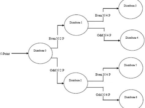
time by using index. In our program, we store 32 twiddle factors for using different versions of algorithm for the range 8 point to 32 point FFT. In this aspect, the twiddle factors are complex variables, so we store 32 real and 32 imaginary values in the design file. Also, we have used decimation-in-time technique for the implementation of radix-2 operation. With this technique at first it uses bit-reversal mechanism for distributing input point and then it performs the butterfly calculations.Fig. 3: N-point FFT bit-reversal sorting of Distribute object
There is no need to reserve one or more processors for the bit-reversal sorting, so by using this mechanism we have saved some execution time. Distribute objects divides the even and odd elements of the input stream. The objects will send a set of even points to its left object as well as a set of
odd points to its right object of the input stream. The final stage will get totally separated even and odd points.
In Figure 3, we have shown that for N-point FFT, in the beginning stage the points are spitted into two new objects with each N/2 points and in the following stage every objects are maintaining the same rule (as was for the first stage) until every processor gets exactly two points.
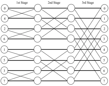
In Figure 4 we have shown an example of mapping and communication through channels for 8 point FFT. For N point FFT the same mapping mechanism will be used. In this figure, each circle represents an object or processor which is running and arrow represents the flow of data. Input stream consists of both real and imaginary parts of the time domain signal.
In our design approach, each object will compute only 2-point butterfly calculations and therefore all objects will get the same work load. Because of having the same work load, processor stalls are reduced in this design. This design does not require any change in the clock frequency of objects or processors. Figure 4 shows three butterfly stages where each object gets 2 point from distribute objects and perform the butterfly computations throughout the butterfly stages. The twiddle factors are used in butterfly computations which supplied either through design file or compute at runtime by using another algorithm. In our implementations, we have sent twiddle factors through design file in run time. After butterfly computations, the output samples collected and assembled by assembler objects A1, A2, A0 and then the
[image:4.595.51.288.518.694.2]final result will send to the output file.
Fig. 4: 8-Point FFT Design Approach
Since our design is parameterized version, channel connection between two processors has to be established automatically during compile time and make a proper design for a specific version of FFT. The distribute objects and assembler objects have the same way of connecting one processor to another. The distribute object D0 will distribute
the samples in two ways and send it to the next stage distribute objects D1, D2 for further process. So, every
as the finalFFT are connected between RealFFTs and assembler objects. According to our design if we consider 8-point FFT, so that we need a total of 18 objects, the 3 objects for distribute, 3 objects for assembleand 12 objects for butterfly computation. Similarly, for 16-point FFT we require a total of 46 objects.
In general for N-point FFT,
Numbers of SR processors = 2(N/m-1) ……… (2) Number of SRD processors = (N/m log2N) …. …… .(3)
The Total number of Processor =
N
m
1
N
m
log
2
N
2
…………. ……. (4)Where m is the number of points calculating on each object and should be the power of 2. N is the total number of points in the FFT and Log2 (N) represents number of stages in the FFT.
If we want to calculate the larger number of FFT points, the total numbers of processors are required to increase gradually. The Am2045 processor has a total of 336 processors and half of them are SR (Streaming RISC) processor. So, we have only 168 SRD processors available to calculate butterfly operations, since we cannot use SR processors for the multiplication. In our design, we consider two points calculation in one object, so that we can only implement this design for the range of 8 to 32-point FFT. However, if we want calculating larger FFT point by using this design, we have to increase the number of point calculation on each object that means the value of m in the equation (4). By following this technique we will be able to use this design for calculating any number of FFT points with in the design constraints.
B. Performance Testing Tools
The PerfHarness tools released in July, 2010 by the Ambric providers Nethra Imaging Inc. By using these tools, we found the performance in terms of latency and cycle count per output sample for different versions of FFT algorithm. Here the term Latency means the response time for the first output for a given first input. And the cycle count per output sample indicates the clock cycles between two workload results. In this test, the ddrLoader Object reads the input samples and stores in DDR memory from input file. The PerfHarness Object streams the input samples from the DDR memory and calculates the performance. After that in the next stage the full program will be loaded in to the dut Object. After completing algorithm’s execution the output will return back to the PerfHarness Object where it finds the latency and cycle count per output sample as shown in the below Fig. 5.
VI. FFTRESULT ANALYSIS
[image:5.595.304.550.169.310.2]The table 1 shows the results of FFT where we displayed the latency, cycle count and number of processors required in different complexity of algorithms like 8 point, 16 point and 32 point FFT. We have collected required number of SRD and SR processors and cycle count per output sample by using PerfHarness tools. For calculating the latency of FFT algorithm we have used performance analyzer which is attached with the aDesigner simulator.
Table 1: Results for FFT FFT Results
FFT By 8 Points 16 Points 32 Points
Design Perf Harness Total
By Design
Perf Harness Total
By Design
Perf Harness Total
SRD
Processors 12 6 18 32 6 38 80 6 86
SR
Processors 6 24 30 14 24 38 30 24 54
Latency
(cycles) 979 2643 4254
Cycle Count/ Output Sample
377 234 197
As shown in the table 1, design for 8 point FFT requires 12 SRD processors that we can verify from the equation (3), but in fact it requires a total of 18 SRDs. That means 6 of those 18 SRD processors are used by PerfHarness tools. This situation will remain same for all other design cases of different point FFT. According to our design in 8 point FFT every SRD object will work on two input points. For this purpose we have to distribute 8 points until every processor gets two input samples. For distribution purpose we require three SR processors since they do not perform any arithmetic operations. After distributing the input samples it has to be sent to the next processors where they are performing butterfly calculations. Here we require three stages with four set of SRD processors which can perform arithmetic operations, because they can execute DSP instructions. Therefore, we use a total of 12 SRD for 8 point FFT. When the arithmetic operation is performed, the results are assembled and sent to the design output. At this Assembler stage, we require three more SR processors for assembling the results which are coming from the butterfly (FFT) stage. Therefore, a total of 12 SRD and 6 SR processors are required for 8 point FFT algorithm mapping. However, there are 30 SR processors are used by the design of 8 point FFT where we need only 6 SR processors for performing distribution and accumulation of data and the remaining 24 SR processors are used by the PerfHarness tools to do performance test.
When the complexity of algorithm increases, the number of processors required will increase, because we consider two points butterfly calculation for each and every SRD processor. So, for 16 point FFT, it requires 32 SRD and 14 SR processors. Similarly, for 32 point, more processors are required than 16 point. It is because when number of point increases, the design requires more SR and SRD processors. The SR processors are used for distributing input samples and assembling the output samples and the SRD processors are used for performing butterfly operations.
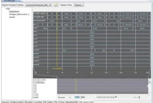
[image:5.595.48.288.673.716.2]can be found by using performance analyzer tool which is embedded within the aDesigner simulator. This analyzer is mainly used to analyze code efficiency rather than to analyze the application in run time. It allows the programmer to evaluate only single processors by giving some cycle counts as total cycle count. The total number of cycle counts is equal to the number of instructions executed plus the number of processor stalls. Whenever a processor is waiting for an input or output (waiting for other processor to get input from it) is known as stall. This analyzer cannot analyze both composite objects and applications. In addition to the total cycle counts, the analyzer gives also the data in the registers like inputs, outputs and program counter with the first and last cycle numbers of duration of data transfer. For example, between 5th cycle and 13th cycle there is a
Hexadecimal number 0x10000 in the first input and output. When finding individual latency for each processor, the first processor distribute_00 of 8 point FFT, we got 8 cycles. In the next stage, where two processors are in parallel, we consider the processor having maximum latency to add with the serial processor of previous stage. Similarly, in further stages, we have to also find out the execution time for all parallel connected objects and the processor with the maximum number of latency is considered. This maximum latency would be added to the previously calculated execution time. This cumulative addition of execution time of individual objects gives the total latency of the entire application.
Here the analyzer ignores the channel stalls which mean that it does not count the cycles when the processor waits for an input or when it waits to send an output. The length of a cycle in seconds can change from a processor to processor, as the processors can run with their own different frequencies. So, when a processor counts two cycles, the another one may count more than two for three cycles in the same time, depending on the frequencies of the processor. When there is any negative value in any register, the performance analyzer shows it as 0x7fffffff. This becomes a serious problem for analyzing it in an accurate way.
As shown in the table 1, the latency increases with algorithm complexity because when we increased FFT points, we need more number of processors for distribute the input samples, butterfly computations and assembling all the output samples. For more butterfly computations the instructions to be executed by the processor obviously will be more and also processor stall will be more. Thus, the
overall latency will also increase. For 16 point FFT the latency is more than double compared to 8 point FFT. In case of 32 point FFT, the latency is approximately less than double compared to 16 points, which is due to the less number of processor stalls. If we compare the complexity with respective to latency, we can observe that 32 point FFT is running more efficiently.
The cycle count per output sample for different point of FFT is shown in the table 1. As we have already discussed above, the cycle count for 8 point FFT is 377 cycles and for every 377 cycles it can receive one output sample for the case of 8 point FFT. When the complexity increases, the cycle count will be decreased because we increase FFT point and so the work loads on each processor. This increase keeps all processors busy so that the processor stalls decreases as shown in table 1.
VII. CONCLUSION
The main aim of this work is to develop a parameterized version FFT algorithm of complex input variables which should work for multiple ranges of complexities. This parameterized version of FFT algorithm works from 8 point to 32 point for given parameter values in the program, which is designed specifically for Radar Signal Processing applications where the input variables are complex variables. Since the aDesigner do not support floating point operations, we solved this problem by converting Floating point data to fixed point representation. In our implementation, we provided the coefficients needed in different ways, such as by using lookup tables, by storing coefficients in external memory provided to processor in run time through input streaming and also by passing the objects at compile time. The coefficients are provided to the design file so that the algorithm can access this coefficient in run time. Higher order FFT filters is able to sample the data at higher rate which permits the user to specify larger order of filters without compromising maximum attainable clock speed. We performed the simulation of FFT algorithm by using PerfHarness tools which provided by Nethra Inc. Using these tools we collected the simulated output in terms of latency and cycle count per output sample. This paper shows that the architecture of MPPA which is suitable for parameterized versioned algorithm FFT.
REFERENCES
[1] Robert J. Purdy, Peter E. Blankenship, Charles Edward Muehe, Charles M. Rader, Ernest Stern, and Richard C. Williamson, Radar Signal Processing, volume 12, number 2, 2000 Lincoln laboratory journal.
[2] E. Chu, A. George, “Inside the FFT black box Serial and parallel fast fourier transfor algorithms”, CRC Press, 2000.
[3] B. Bylin and R. Karlsson, “Extreme processor for extreme
processing”, Technical Report, Halmstad University, IDE0503, January 2005.
[4] S. Jenkins “MIMO/OFDM Implement OFDMA, MIMO for WiMAX,
LTE”, picoChip <http://www.eetasia.com/ARTICLES/2008MAR/PDF/EEOL_2008M
AR17_RFD_NETD _TA.pdf.
[5] P. Söderstam, “STAP Signal Processing Algorithms on Ring and Torus SIMD Arrays”, Technical Report, Chalmers University of Technology. April 1998.
[image:6.595.45.291.390.555.2][6] “Am2000FamilyArchRef_2008_3”,http://ambric.info/documentation/ Documentation/MPPAs/Am2000FamilyArchRef_2008_3.pdf, Date 02-05-2008.