Identification of material damage in two dimensional domains using squid based NDE system

IDENTIFICATION OF MATERIAL DAMAGE

IN TWO DIMENSIONAL DOMAINS

USING SQUID BASED NDE SYSTEM

Abstract

Problems on the identification of two-dimensional spatial domains arising in the detection and characterization of material damage are considered. For electromag-netic nondestructive evaluation systems, observations of the magelectromag-netic flux from the front surface are used in a output least-square approach. Parameter estimation tech-niques based on the method of mappings are discussed and approximation schemes are developed applying a finite-element Galerkin approach. Theoretical convergence results for computational techniques are given and results are applied to numerical experiments to demonstrate the efficacy of the proposed schemes.

1

Introduction

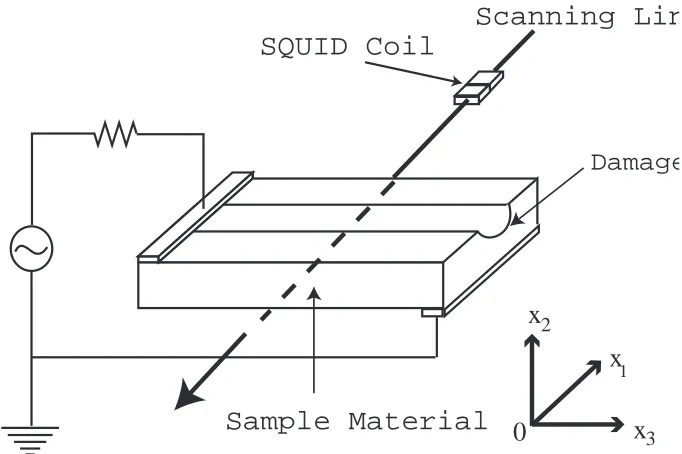
Detection and characterization of small cracks and corrosion embedded in the structures of aircraft are critical issues in the maintenance of aging aircraft. For instance, carbon fiber reinforced plastics (CFRP) have been widely used in the advanced aircraft and, as a result, demand has grown for assessing the structural integrity of structures made from those materials. An important effort on such problems entails quantitative nondestructive evaluation methods in SQUID-based NDE system [1]. It is well known that SQUIDs (su-perconducting quantum interference devices ) have very high sensitivity for magnetic flux measurements. Due to the highly sensitive magnetic flux measurements, inverse analyses on electromagnetic problems are effectively used for detecting and characterizing cracks and delamination. Initial efforts on such inverse problems include nondestructive testing under SQUID measurements using the direct current method [2]. However, the detections of non-through crack and corrosion-like damage by direct current flows are insufficient be-cause of the lack of information for deep-lying effects from vertical component of magnetic flux measurements. Since a skin depth of metal varies according to frequency of flowing current, it is possible to detect the deep-lying flows by controlling the frequency. To this end, SQUID based nondestructive evaluation (NDE) systems using injection current methods have been recently developed [3, 4]. In this paper, we propose a computational method for recovering corrosion-like damage with magnetic flux density data from the SQUID based NDE system with alternating current force. The idea of the method of mapping techniques ([5, 6]) are effectively used in our inversion procedures. Figure 1 illustrates the overall configuration of SQUID based NDE system proposed here. In this 1_{Center for Research in Scientific Computation, North Carolina State University, Raleigh, NC} 27695-8205, USA. E-mail: [email protected]

Sample Material

SQUID Coil

Scanning Lin

Damage

x

x

x

1

2

3

0

Figure 1: Overall Configuration of SQUID based NDE System

inspection procedure, alternating current forces with multiple angular frequencies are ap-plied to the sample material inspected. A damage corrupts the current flows inside the conductor and we can detect this disturbance from the magnetic flux measurements by the SQUID. The task we consider here is to identify the geometrical shape of the damage from input and output data. Throughout the paper, we assume that the damage is lo-cated sufficiently far from both sides of the sample and that the direction of current flow is uniform with respect to the length direction. In Section 2, we consider a two-dimensional mathematical model for inspections based on a SQUID-based NDE system. In Section 3, a direct problem is formulated in variational form in an appropriate Hilbert space. In Section 4, the inverse problem is discussed in the context of a nonlinear output least square problem. The class of admissible parameters are given and the existence of solu-tions is demonstrated using the idea of the method of mappings. Section 5 is devoted to theoretical convergence for the proposed computational method. Numerical experiments are summarized in Section 6 to demonstrate the efficacy of the proposed method. Related efforts on similar problems are given in [7, 8, 9] where eddy current based techniques are used and the focus is model reduction techniques are opposed to the use of the method of maps employed here.

2

Mathematical Model of Inspection Procedures

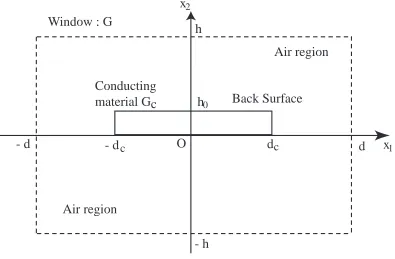
Our forward analysis is considered on a cross section of the conducting material sample, i.e.,

Gc ={ x= (x1, x2)| |x1|< dc, 0< x2 < h0 }

Air region

- d

_d

h

- h

O

h

Conducting

material Gc

Air region

x

x

1 2

Back Surface

Window : G

- d

d

Figure 2: Inspection Area

our problem is defined on an appropriate computational “window” given by G={ _x| |_x1|_{< d,} |_x2|_{< h}(_{h0 < h <} ∞)}_.

A set of alternating current sourcesJ_iwith frequencies_ωiis applied to the sample material J_i(_t,x) = (0_,0_{, Js}(x))T cos(_ωit)_.

The set of applied frequencies _ω={_ωi}M_i=1o can be determined in accordance with the skin depth condition,

δ = s

2

σµω (1)

where_µdenotes the magnetic permeability and where_σdenotes the electrical conductivity of the sample. Given that skin depth of a metal changes according to frequency of flowing current, it is possible to detect a configuration of deep-lying defects by varying the frequency. For the output, measurements can detect the gain margin and phase change of the voltage using a LCZ meter. This means that the SQUID measurements can be represented as

B(_t,x) =B(x) cos(_ωt+_θ(x))_.

Thus it is natural and convenient that the state variables be described by complex phasor representations. The phasor form of Maxwell’s equations is given by

∇ ·E = 0_, (3)

∇ ×E = −_jωB_, (4)

∇ ×H = J_. (5)

Following a standard approach, we introduce the magnetic vector potential A=

(_{Ax1, Ax2, Ax3}) defined by B =∇ ×A and the cross product of Eq. ( 4 ) can be replaced by representing E+_jωA as the gradient of a scalar electrical potential _φ, i. e.,

E=−_jωA− ∇_φ.

In conjunction with Ohm’s law J = _σE and the constitutive law B = _µH, the system state A is governed by

∇ × 1

µ∇ ×A = −jωσA−σ∇φ (6)

∇ ·(_jωA+∇_φ) = 0_. (7)

We assume here that the sample is of nonmagnetic material, so that the magnetic per-meability _µis equal to that of air, i.e., _µ=_µ0. In our formulation, the magnetic vector potential becomes A= (0_,0_{, A3}). Therefore, the equation for the component of magnetic vector potential _A3 =_A is simply rewritten as

− 1

µ0∇

2_A+jχ

cσωA=−χcσ ∂φ ∂x3

where _χc denotes the characteristic function of the conducting region _Gc. Taking into account that the right side of the above equation is composed of the source current density, it follows that

Js=−σ ∂φ

∂x3 inGc.

Consequently we can formulate the two dimensional forward problem in terms of the equation:

− 1

µ0

∂2A(_{x1, x2}) ∂x21

+ ∂

2_A(x 1, x2)

∂x22

!

+_jχcσωA(_{x1, x2}) =_χcJs(_{x1, x2})_. (8)

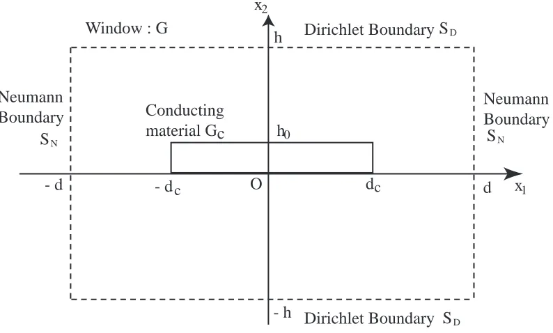
Since the boundaries in the _x2 directions are assumed to be sufficiently far from the sample, we assign a Dirichlet boundary condition on this part of the boundary, i. e.,

A= 0 on _SD (9)

where

SD ={ x | |x1|< d, |x2|=h }.

We also consider the boundaries in the_x1 directions to be sufficiently far from the damage so that Neumann boundary conditions in the _x1 direction can be set as:

∂A

- d _d h

- h O

h0

Conducting material Gc

x x

1 2

Window : G SD

SD

SN SN

Dirichlet Boundary

Dirichlet Boundary Neumann

Boundary

Neumann Boundary

- d_c dc

Figure 3: Setting of the boundary condition on the window

where

SN ={x | |x1|=d, |x2|< h}.

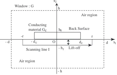
Figure 3 denotes the boundary conditions on the computational window. In contrast to other magnetic sensors, SQUID measurements can directly detect the magnetic flux densities that are independent of the applied frequencies. Suppose that the scanning strategy is given on the line

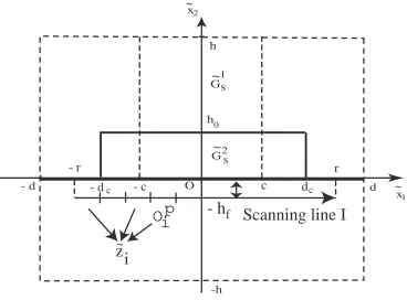
I ={ x∈_G| |_x1| ≤_r (_{dc < r})_{, x2} =−_hf }_, as shown in Fig. 4. Thus the observation mechanism involves data

B2(xp) =−∂A

∂x1(x

p_{) for x}p _{∈I, p= 1,2,· · ·, m. (11)}

and the observations are given by

z =H_A ∈ Cm (12)

where H denotes the bounded operator given by

{H}p = −

1

|Op| Z

Op

∂(·) ∂x1dx1

x2=−hf

(13)

and Op _{denotes the sub-interval ofI defined by}

Op _{⊂ (p= 1,2,· · ·, m). (14)}

Air region

- d

_d

h

- h

- h

O

h

Scanning line I

Conducting

material Gc

Lift-off

Air region

x

x

1 2

f

Back Surface

Window : G

- d

_d

-r

r

Figure 4: Scanning procedures

3

Weak Formulation

Let q be a constant vector which characterizes an unknown damage shape where we assume

[H-0] The admissible set_Q of damage parameters is a compact subset of _RM _.

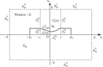
We introduce the “suspect region” _Gs ⊂ _G which covers the suspected but unknown damage. More precisely, as depicted in Fig 5, the domain _Gs is described by

Gs={ x= (x1, x2) | |x1|< c, 0< x2 < h }.

For convenience of discussions, the suspect region _Gs is decomposed into two subre-gions which correspond to the air region _G1_s and the conducting region _G2_s and these are parametrized by q. Thus the “window” _G is decomposed into three sub-regions _G0, G1_s and _G2_s as follows:

Gs =G1s(q)∪Gs2(q), G0 =G−Gs.

We assume the boundary of _G is decomposed into S_N0 = {x | |_x1|=_d, |_x2| ≤_h }

- d

_d

h

- h

O

h

x

x

1 2

Window : G

G1

G2

S

S

S

S12_I(q)

(q)

(q)

0

S

0

S

S

S01_I S01_I

S02_I S02_I

S02_I

G

- d

- c

d

s

s

Figure 5: Domain decomposition

and that the interface among sub-regions are defined by S_I01 = {x| |_x1|=_{c, h0} ≤_{x2 < h}}

SI02 = {x| |x1|=c, 0< x2 < h0 } ∪ {x| |x1| ≤c, x2 = 0 }

and _SI12 is defined by the interface between _G1_s(q) and _G2_s(q). The form of _SI12 will be described in the later discussions. The system state is then denoted by

A:=_A0 in _{G0 A}:=_Ai in _Gi_s (_i= 1_,2) where

Ai :=ARi +jAiI (i= 0,1,2).

In the sequel, we suppose that the electric conductivity of the conducting material sample has constant value_σc, i.e.

σ=_χcσc. Thus the subsystem on _G0 is described by

− 1

µ0∇ 2_AR

0 −χcσcωAI0 = χcJs (15)

− 1

µ0∇ 2_AI

with the boundary condition

AR₀ =_AI₀ = 0 on _SD0 (17)

∂AR

0

∂n = ∂AI

0

∂n = 0 on S

0

N. (18)

The subsystems defined on _G1_s(q) and _G2_s(q) are described respectively by

∇2_AR

1 = 0 (19)

∇2_AI

1 = 0 in G1s(q) (20)

with the boundary condition

AR1 =AI1 = 0 on SD1, (21)

and

− 1

µ0∇ 2_AR

2 −σcωAI2 = Js (22)

− 1

µ0∇ 2_AI

2 +σcωAR2 = 0 in G2s(q). (23)

We also need the interface conditions between _G0,_G1_s(q), and_G2_s(q),

AR₀ −AR₁ =_AI₀−_AI₁ = 0 (24)

∂AR 0 ∂n − ∂AR 1 ∂n = ∂AI 0 ∂n − ∂AI 1

∂n = 0 on S

01

I (25)

AR₀ −AR₂ =_AI₀−_AI₂ = 0 (26)

∂AR 0 ∂n − ∂AR 2 ∂n = ∂AI 0 ∂n − ∂AI 2

∂n = 0 on S

02

I (27)

AR₁ −AR₂ =_AI₁−_AI₂ = 0 (28)

∂AR 1 ∂n − ∂AR 2 ∂n = ∂AI 1 ∂n − ∂AI 2

∂n = 0 on S

12

I (q). (29)

Let _ϕ be in the set

Vq ={ ϕ ∈H1(G0∪G1s(q)∪G2s(q))| ϕ = 0 onSD0 ∪SD1 }

endowed with the norm

kϕk2 := ZZ

G0∪G1s(q)∪G2s(q)

|∇ϕ|2dx1dx2.

Let us set

~

ϕ:= (_ϕR_{, ϕ}I)∈_Vq×_Vq.

Then, for any _{ϕ, ~~ ψ} ∈_Vq×_Vq, we define the bilinear form on _Vq×_Vq a(q)(_{ϕ, ~~ ψ}) := 1

µ0

ZZ

G0∪G1s(q)∪G2s(q)

∇ϕR· ∇ψR+∇_ϕI · ∇_ψI_dx1dx2

−ω ZZ

G0∪G2s(q)

χcσcϕIψRdx1dx2

+_ω ZZ

G0∪G2s(q)

and the linear form on _Vq

L(q)(_ϕ~) := ZZ

G0∪G2s(q)χcJsϕ

R_dx

1dx2. (31)

Lemma 1: Suppose that

[H-1]: The applied angular frequency _ω is properly chosen such that ω≤ω0 <∞

and that

χcJs∈L2(G).

Then, for every q∈_Q, there exists a unique solution _A~(q) = (_AR_{, A}I₎∈_V

q×Vq which is

the solution of

a(q)(_{A, ~}~ _ϕ) =_L(q)(_ϕ~) for _ϕ~ ∈_Vq×_Vq. (32) Moreover, we have

k_A~(q)k_Vq×Vq ≤_K1k_χcJsk_L2_(G) (33)

where _K1 is a constant independent ofq.

Proof: For arbitrary _ϕ~ ∈_Vq×_Vq, _a(q) is _Vq×_Vq-elliptic with constant _δ= 1_/µ0 since

a(q)(_{ϕ, ~~ ϕ}) = 1 µ0

ZZ

G0∪G1s(q)∪G2s(q)

∇ϕR2+∇ϕI2

dx1dx2 =δkϕ~k2Vq×Vq (34)

from which follows the coercivity. For the boundedness, it can be easily checked that

a(q)(_{ϕ, ~~ ψ})≤γkϕ~k_Vq×Vqψ~

Vq×Vq. (35)

The linear functional _L(q) is bounded on_Vq×_Vq, i.e.,

|L(q)(_ϕ~)| = ZZ

G0χcJsϕ

R_dx

1dx2+

ZZ

G2s(q)

JsϕRdx1dx2

≤ ZZ

G0

χcJsϕRdx1dx2+ ZZ

G2s(q)

JsϕRdx1dx2

≤

  

ZZ

G0|χcJs|

2

dx1dx2

1 2

+ ZZ

G2s(q)

|Js|2dx1dx2 !1

2



×kϕ~kL2(G0∪G1s(q)∪G2s(q))

≤ Mkϕ~k_Vq×Vq for _ϕ~ ∈_Vq×_Vq.

Applying the Lax-Milgram lemma, for eachq∈_Q, we find there exists a unique solution ~

A(q)∈_Vq×_Vq satisfying (32). Similarly, we have

- d

_d

h

- h

O

h

x

x

1 2

Window : G

G1

G2(q)

(q)

G

- d

- c

d

r(x ; q)

s

s

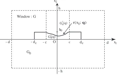
Figure 6: The unknown damage function

from which follows

k_A~(q)k_Vq×Vq ≤_K1 where _K1 = M δ . This completes the proof.

Remark: In [H-1], the upper bound of angular frequency _ω0 can be reasonably set for the inspection. More precisely, the angular frequency _ω of the applied current force must be properly chosen by the skin depth condition (1).

4

Admissible Class and Method of Mapping

In this section, we restrict the corrosion-like damage so that it can be represented by a simple parametrized function. The unknown defect shape is characterized by a function

x2 =r(x1;q) for |x1| ≤c (36)

with

0_{< r}(_x1;q)≤_h0 ( _{< h <}∞ ) and _r(−_c;q) =_r(_c;q) =_h0

as depicted in Fig. 6. We describe by _Q ⊂ _RM _{an admissible set of possible parameter}

- d

_d

h

- h

O

h

x

x

1 2

Window : G

G1

G

- d

- c

d

s

~

G

~

Figure 7: Refence domains

[H-3] There exists a constant_β such that, for each q∈_Q, 0_{< β} ≤_r(·_,q)_.

[H-4]There exists a function_dist:_Q×_Q→_R1 with _dist(q_,q)˜ →0 as |q−q˜| →0 such that

kr(·_,q)−_r(·_,q)˜ k_1,∞≤_dist(q_,q)˜ for q_,q˜ ∈_Q.

The subregions _G1(q) and _G2(q) given in the previous section can now be explicitly rewritten as

G1_s(q) ={ x| |_x1|_{< c, r}(_x1,q)_{< x2 < h}} and

G2_s(q) = { x| |_x1|_{< c,} 0_{< x2 < r}(_x1,q) }_,

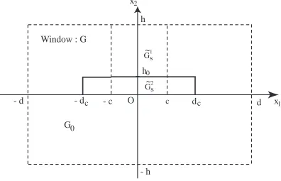
respectively. Associated with these sub-domains, we define the reference sub-domains as shown in Fig. 7:

˜

G1_s ={ x| |_x1|_{< c, h0 < x2 < h} } ˜

G2s ={ x| |x1|< c, 0< x2 < h0 }.

We introduce the affine mapping:

x=_T(q)˜_x= (

T1(q)˜x for ˜x∈G˜1s T2(q)˜x for ˜x∈G˜2s

h

O

x

x

1 2

- c

c

r(x ; q)

h

G

(q)

G

(q)

h

O

x

x

1 2

- c

c

h

G

G

~

~

T(q)

~

~

s

s

s

s

Figure 8: Transformation mapping from the reference domain into the domain with dam-age

where

T1(q) =

(

x1 = ˜x1

x2 = (h−r(˜x1;q))(˜x2−h)/(h−h0) +h

T2(q) =

(

x1 = ˜x1

x2 = r(˜x1;q)˜x2/h0 .

These mappings result in the following identities :

Gis(q) =Ti(q)◦G˜is (i= 1,2). (38)

Figure 8 illustrates the transformation from the reference domain ˜_G1_s∪_G˜2_s into the domain with damage_G1_s(q)∪_G2_s(q). Let ˜_ϕ be in the set

˜

V ={ _ϕ˜∈_H1(_G0∪_G˜1_s∪_G˜2_s) |_ϕ˜= 0 on _SD0 ∪_SD1 } endowed with the norm

k_ϕ˜k2 := ZZ

G0∪G˜1s∪G˜2s

|∇_ϕ˜|2_dx˜_1dx˜_2.

Let us set

~˜

ϕ:= ( ˜_ϕR_,ϕ˜I)∈_V˜ ×_{V .}˜

Then, for any _{ϕ, ~}~˜ _ψ˜∈_V˜ ×_V˜, the bilinear form _a(q) can be represented on ˜_V ×_V˜ as

˜

a(q)(~_{ϕ, ~}˜ _ψ˜) := 1 µ0

2

X

i=1 ZZ

˜

Gis

˜

∇_ϕ˜R

·_∇˜_T

i(q) _−t

˜

∇Ti(q) ₋₁

˜

+∇˜_ϕ˜I·∇˜_Ti(q)−t∇˜_Ti(q)−1∇˜_ψ˜Idet∇˜Ti(q)dx˜1dx˜2 + 1 µ0 ZZ G0 n ˜

∇_ϕ˜R·∇˜_ψ˜R+∇˜_ϕ˜I·∇˜_ψ˜Io_dx˜_1dx˜₂

−ω ZZ

˜

G2s

σcϕ˜Iψ˜Rdet∇˜T2(q)dx˜1dx˜2

+_ω ZZ

˜

G2s

σcϕ˜Rψ˜Idet∇˜T2(q)dx˜1dx˜2

−ω ZZ

G0χcσc

˜

ϕIψ˜Rd_x˜_1dx˜₂ +_ω ZZ

G0χcσc

˜

ϕRψ˜Id_x˜_1dx˜_2. (39)

The linear form on ˜_V is also represented by ˜

L(q)(~_ϕ˜) := ZZ

˜

G2s

Jsϕ˜Rdet∇˜T2(q)dx˜1dx˜2+ ZZ

G0χcJs

˜

ϕRd_x˜_1dx˜_2. (40)

Noting that

˜

∇Ti(q) =   

∂x1

∂˜x1

∂x1

∂x˜2

∂x2

∂˜x1

∂x2

∂x˜2

  ,

we obtain

˜

∇T1(q) =

  

1 0

−r0(˜x1;q)(˜x2−h) h−h0

h−r(˜x1;q)

h−h0

 

 ∇˜T2(q) =

  

1 0

−r0(˜x1;q)˜x2

h0

r(˜x1;q)

h0

  .

Similarly, we have

det∇˜T1(q)= h−r

(˜_x1;q) h−h0 det

∇˜T1(q)= r

(˜_x1;q) h0 .

Hence the explicit form of Eq. (39) can be represented as

˜

a(q)(~_{ϕ, ~}˜ _ψ˜) :=

2

X

i=1 ZZ

˜

Gis

(

ai₁(q) ∂ϕ˜

R ∂_x˜₁

∂ψ˜R ∂_x˜₁ +

∂_ϕ˜I ∂_x˜₁

∂ψ˜I ∂_x˜₁

!

+_ai₂(q) ∂ϕ˜

R ∂_x˜₁

∂ψ˜R ∂_x˜₂ +

∂_ϕ˜R ∂_x˜₂

∂ψ˜R ∂_x˜₁ +

∂_ϕ˜I ∂_x˜₁

∂ψ˜I ∂_x˜₂ +

∂_ϕ˜I ∂_x˜₂

∂ψ˜I ∂_x˜₁

!

+_ai₃(q) ∂ϕ˜

R ∂_x˜₂

∂ψ˜R ∂_x˜₂ +

∂_ϕ˜I ∂_x˜₂

∂ψ˜I ∂_x˜₂

!)

d_x˜_1dx˜₂

+1 µ0

ZZ

G0

∂_ϕ˜R ∂_x˜₁

∂ψ˜R ∂_x˜₁ +

∂_ϕ˜I ∂_x˜₁

∂ψ˜I ∂_x˜₁ +

∂_ϕ˜R ∂_x˜₂

∂ψ˜R ∂_x˜₂ +

∂_ϕ˜I ∂_x˜₂

∂ψ˜I ∂_x˜₂

!

d_x˜_1dx˜₂ +

ZZ

˜

G2sa0

(q)−_ϕ˜I_ψ˜R+ ˜_ϕR_ψ˜I_dx˜_1dx˜₂ +_ω

ZZ

G0χcσc

−_ϕ˜I_ψ˜R+ ˜_ϕR_ψ˜I

where

a11(q) = r

0_(˜x

1;q)2(˜x2 −h)2+ (h−r(˜x1;q))2

µ0(h−h0)(h−r(˜x1;q))

a1₂(q) = r

0_(˜x

1;q)(˜x2 −h)

µ0(h−r(˜x1;q))

a1₃(q) = h−h0 µ0(h−r(˜x1;q))

a21(q) = r

0_(˜x

1;q)2x˜22+r(˜x1;q)2

µ0h0r(˜x1;q)

a22(q) = −r

0_(˜x

1;q)˜x2

µ0r(˜x1;q)

a2₃(q) = h0 µ0r(˜x1;q),

and where

a0(q) = ωσcr(˜x1;q)

h0 .

From (40), the transformed linear form can be explicitly rewritten by

˜

L(q)(~_ϕ˜) := ZZ

˜

G2s

Jsr(˜x1;q) h0 ϕ˜

R_dx˜

1dx˜2+

ZZ

G0χcJs

˜

ϕRd_x˜_1dx˜_2. (42)

Lemma 2: With the hypotheses [H-0] to [H-4], there exist positive constants _{α, λ, K2} and _K3 such that, for q_1,q₂ ∈ _Q, the bilinear form ˜_a(q)(·_,·) satisfies the following in-equalities for all ~_{ϕ, ~}˜ _ψ˜∈_V˜ ×_V˜:

˜

a(q)(~_{ϕ, ~}˜ _ϕ˜) ≥ _α~_ϕ˜2_˜

V×V˜ (43)

_a˜(q)(~_{ϕ, ~}˜ _ψ˜) ≤ _K2~_ϕ˜_˜ V×V˜

_ψ~˜

˜

V×V˜

(44)

˜_a(q)(~_{ϕ, ~}˜ _ψ˜)−_a˜(˜q)(~_{ϕ, ~}˜ _ψ˜) ≤ _K3dist(q_,q)˜ ~_ϕ˜_˜ V×V˜

~_ψ˜

˜

V×V˜

(45)

where

dist(q_,q)˜ →0 as |q−q˜| →0_.

Moreover, _α, _K2, and _K3 can be chosen as constants which are independent of the pa-rameter vector q.

Proof: It can be easily shown that, with _{c1, c3 >}0, any quadratic form satisfies

c1(ξ1)2−2c2ξ1ξ2+c3(ξ22)≥ c1c3−

(_c2)2

2 min

n

From (41), the associated quadratic form for each suspect region _Gi

s(i= 1,2) becomes n

a1i(q)(ξ1R)2+ 2ai2(q)(ξ1Rξ2R) +ai3(q)(ξR2)2

o

+ n_ai₁(q)(_ξ1I)2+ 2_ai₂(q)(_ξ1I_ξ2I) +_ai₃(q)(_ξ2I)2o

≥ ai1(q)ai3(q)−(ai2(q))2

2 min

n

(_ai₁(q))−1_,(_ai₃(q))−1o

×(|_ξ1R|2 +|_ξ2R|2+|_ξI₁|2+|_ξ2I|2)_. (46) We easily find that

ai₁(q)_ai₃(q)−(_ai₂(q))2 = 1 for _i= 1_,2_. Under the hypotheses [H-2]and [H-3], we admit that

(_a1₁(q))−1 = µ0(h−h0)(h−r(˜x1;q))

r0(˜_x1;q)2(˜_x2−_h)2+ (_h−_r(˜_x1;q))2 ≥ µ0

M1+M2

(_a1₃(q))−1 = µ0(h−r(˜x1;q)) h−h0 ≥µ0

where

M1 = sup q∈Q

sup

x1∈[−c,c]

|r0(˜_x1;q)|2 _M2 = h−β h−h0

!₂

≥1_.

This implies that, for_G1_s,

minn(_a1₁(q))−1_,(_a1₃(q))−1o≥ µ0

M1+M2. (47)

Similarly, noting that

(_a2₁(q))−1 = µ0h0r(˜x1;q)

r0(˜_x1;q)2_x˜2₂+_r(˜_x1;q)2 ≥

µ0β

h0(M1+ 1)

(_a2₃(q))−1 = µ0r(˜x1;q)

h0 ≥

µ0β

h0 ,

we obtain

minn(_a2₁(q))−1_,(_a2₃(q))−1o≥ µ0β h0(M1+ 1)

for _G2_s. (48) Choosing the constant as

α= min (

µ0

M1+M2,

µ0β

h0(M1+ 1),

1 µ0

)

which is independent of q, we obtain the coercivity (43) of the transformed sesquilinear form. To prove the boundedness, we note that, under the hypotheses [H-1] to [H-4], it follows that

ai_j(q) ≤  sup

q∈q

sup

˜

Gis

ai_j(q)2  

1 2

(=_M2) for _i= 1_,2;_j = 1_,2

ai3(q) ≤ max

(

h−h0

µ0(h−β),

h0

µ0β

)

(=_M3) for _i= 1_,2

Thus, by setting as

K2 = max

M2, M3, M4, µ−01

,

we obtain the boundedness (44). To establish the continuity property, we note that, for any q_,q˜∈_Q,

˜_a(q)(~_{ϕ, ~}˜ _ψ˜)−˜_a(˜q)(~_{ϕ, ~}˜ _ψ˜)

≤ X2

i=1 ZZ ˜

Gis

"n

ai1(q)−ai1(˜q)

o _∂ϕ˜R ∂_x˜₁

∂ψ˜R ∂_x˜₁ +

∂_ϕ˜I ∂_x˜₁

∂ψ˜I ∂_x˜₁

!

+n_ai₂(q)−_ai₂(˜q)o ∂ϕ˜

R ∂_x˜₁

∂ψ˜R ∂_x˜₂ +

∂_ϕ˜R ∂_x˜₂

∂ψ˜R ∂_x˜₁ +

∂_ϕ˜I ∂_x˜₁

∂ψ˜I ∂_x˜₂ +

∂_ϕ˜I ∂_x˜₂

∂ψ˜I ∂_x˜₁

!

+n_ai₃(q)−_ai₃(˜q)o ∂ϕ˜

R ∂_x˜₂

∂ψ˜R ∂_x˜₂ +

∂_ϕ˜I ∂_x˜₂

∂ψ˜I ∂_x˜₂

!#

d_x˜_1dx˜₂

+ ZZ

˜

G2s

{a0(q)−a0(˜q)}

−_ϕ˜I_ψ˜R+ ˜_ϕR_ψ˜I_dx˜_1dx˜_2.

With the hypotheses [H-1] to[H-4], it can be argued that _ai_j(q)(_i= 1_,2;_j = 1_,2_,3) are continuous in _L∞( ˜_Gi

s). We can thus infer the continuity of the bilinear form (41) with

respect to q∈_Q. The proof has been completed. Lemma 3: Let

~˜

A(q) =_A~◦_T(q)

be the transformed system state. Then, with the hypotheses [H-0] to [H-4], for every q∈_Q, there exists a unique solution

~˜

A(q)∈_V˜ ×_V˜ (49)

in the sense that

˜

a(q)(_A~˜(q)_{, ~ϕ}˜) = ˜_L(q)(_ϕ~˜) for ~_ϕ˜∈_V˜ ×_{V .}˜ (50) Moreover the solution _A~˜(q) in the system on _G = _G0 ∪_G˜1_s ∪_G˜2_s is bounded in ˜_V ×_V˜ uniformly inq∈_Q.

Proof: FromLemma-2and from (30), (31), (41), and (42), we have that, for_ϕ~ ∈_Vq×_Vq and ~_ϕ˜∈_V˜ ×_V˜,

α~_ϕ˜2_˜

V×V˜ ≤ |a(q)(ϕ, ~~ ϕ)| ≤K2 ~_ϕ˜2_˜

V×V˜

and

a(q)(_{ϕ, ~~ ϕ}) = ˜_a(q)(~_{ϕ, ~}˜ _ϕ˜)_.

Taking into account that the constants_αand_K4 are independent of the unknown param-eter q, this implies that the _Vq×_Vq-norm is equivalent to the norm of ˜_V ×_V˜ uniformly in q∈_Q. Since, under the hypothesis (H-1),

_L˜_{(q)(~ϕ˜)≤K4~ϕ˜}

there exists the solution ~_A˜in ˜_V ×_V˜ in the sense of (50). The proof has been completed. Lemma 4: With the hypotheses [H-0] to [H-4], q → _A~˜(q) is continuous from _Q to

˜ V ×V˜.

Proof: Let qk → _{q in Q and let A}~˜_(qk_), ~_A˜_{(q) be the corresponding solutions of (50).}

Then, from (50), we have

˜

a(qk)(_A~˜(qk)_{, ~ϕ})−˜_a(q)(_A~˜(q)_{, ~ϕ}) = [ ˜_L(qk)−_L˜(q)](_ϕ~) for ∀_ϕ~ ∈_V˜ ×_{V .}˜ Then we may rewrite

˜

a(qk)(_A~˜(qk)−_A~˜(q)_{, ~ϕ}) + [˜_a(qk)−˜_a(q)](_A~˜(q)_{, ~ϕ}) = [ ˜_L(qk)−_L˜(q)](_ϕ~) for ∀_ϕ~ ∈_V˜ ×_{V .}˜

Choosing as _ϕ~ =_A~˜(qk)−~_A˜(q) in ˜_V ×_V˜ and using (43) and (45) in Lemma-2, we find that

α|A~˜(qk)−_A~˜(q)|2_V˜×V˜ ≤_dist(qk_,q)

|χJs|L2(G)+|A~˜(q)|2_V˜_×V˜

|_A~˜_(qk_)−A~˜_(q)|˜

V×V˜.

This yields the desired continuity, that is,

α|A~˜(qk)−_A~˜(q)|_V˜×V˜ ≤ _dist(qk_,q)

|χJs|L2(G)+|A~˜(q)|2_V˜_×V˜

−→ 0 asqk →q_.

The proof has been completed.

The observation for the transformed state _A~˜can be rewritten by ˜

z(q;_ω) = ˜H_A~˜(q;_ω) (51) where ˜H: ˜_V ×_V˜ →_Rm_×Rm _{is given by}

h ˜

H~_ϕ˜i

i = −

1

|Op| Z

Op

∂_ϕ˜R ∂_x˜₁ ,

∂_ϕ˜I ∂_x˜₁

! d_x˜₁

˜

x2=−hf

(_p= 1_,2_,· · ·_{, m})_.

Figure 9 depicts the procedures for gathering the measurement data from SQUIDs. Lemma 5: With the hypotheses [H-0] to [H-4], the mapping q → _z˜(q) is continuous from_Q to _Rm×_Rm_.

Proof: Taking into account that the operator ˜H belongs to L( ˜_V ×_V˜;_Rm×_Rm) for each q∈_Q, we see that the above statement follows directly from Lemma-4.

- d d h

O

x x

1 2

h

0

-h G 2 G

1

~

~ ~

~

Scanning line I

- h

Oi

p

z

_i

s

s

c - c

- d_c dc

- r r

Figure 9: Data acquisition by SQUIDs

Shape Identification Problem SIDP:

Given the observed data{_zd(_ωi)}M_i=1o from applying the set of alternating injection currents

{Jscos(ωit)}iM=1o, then find the optimal q=q∗ which minimizes the fit-to-data functional

F(q) = 1 2

Mo

X

i=1

_z˜(q;_ωi)−_zd(_ωi)2 (52)

with respect to q∈_Q where _Qis a compact set of _RM_.

Theorem 1: With the hypotheses [H-0] - [H-4], the problem SIDP has at least one solution q∗ ∈_Q.

This follows immediately from the continuity properties given in Lemma 5 and the compactness of Q.

5

Computational Method and Convergence Analysis

The computational scheme is based on the use of a finite Galerkin approach to construct a sequence of finite dimensional approximating identification problems. To approximate SIDP, we choose a sequence of finite dimensional subspace _HN_×HN _⊂V˜_×V˜ _{such that}

ΠN_ϕ~−_ϕ~˜

V×V˜ −→0 as N → ∞ for ϕ~ ∈

˜

where ΠN _{is the orthogonal projection of}

˜

L2(_G0∪_G˜1_s∪_G˜2_s)×_L˜2(_G0∪_G˜1_s∪_G˜2_s) onto _HN ×_HN (54)

The approximating system is defined for_A~˜N ∈_HN _×HN _by

˜

a(q)(_A~˜N_{, ~ϕ}˜N) = ˜_L(q)(_ϕ~˜N) for ~_ϕ˜N ∈_HN ×_HN_. (55) The observation output for the approximating system can be represented as

˜

zN(q;_ω) = ˜H_A~˜N(q;_ω)_. (56) Thus the computational method is formulated as follows:

Approximate Shape Identification Problem (ASIDP)N:

Find ˆqN _{∈Q which minimizes}

FN(q) = 1 2

Mo

X

i=1

_z˜N(q;_ωi)−_zd(_ωi)2 (57)

Lemma 6: LetqN →_q∈_{Q. Then} ~˜

AN(qN)−→_A~˜(q)∈_V˜ ×_{V .}˜ (58)

Proof: We have

A~˜

N

(qN)−_A~˜(q) _˜

V×V˜

≤_A~˜N_(qN_)−ΠN_A~˜_{(q) ˜}

V×V˜

+ΠN_A~˜(q)−_A~˜(q)

˜

V×V˜ .

From (53), it suffices to prove

A~˜

N

(qN)−ΠN_A~˜(q) _˜

V×V˜

→0 for qN →q∈ _Q as _N → ∞_.

We obtain

˜

a(qN)(_A~˜N(qN)_{, ~ψ}N)−˜_a(q)(_A~˜(q)_{, ~ψ}N) = [ ˜_L(qN)−_L˜(q)](_ψ~N) for_ψ~N ∈_HN ×_HN_. Furthermore we have

˜

a(qN)(_A~˜N(qN)−ΠN_A~˜(q)_{, ~ψ}N) + ˜_a(qN)(ΠN_A~˜(q)−_A~˜(q)_{, ~ψ}N)

Choosing _ψ~N _{= ∆}N _=A~˜N_(qN₎−_ΠN~_A˜_{(q), we find that}

α∆N2_˜

V×V˜ ≤ K2

ΠN_A~˜(q)−_A~˜(q)

˜

V×V˜ k

∆Nk_V˜×V˜

+_dist(qN_,q)~_A˜(q)

˜

V×V˜ k

∆Nk_V˜×V˜ +_Mdist(qN_,q)k∆Nk_V˜×V˜.

Consequently, we obtain

α∆N_˜

V×V˜ ≤K2

ΠN_A~˜(q)−_A~˜(q)

˜

V×V˜

+_dist(qN_,q) _A~˜(q)

˜

V×V˜

+_M !

.

Thus, given any qN _{→q∈Q, it follows that ∆}N _{→0 as N → ∞.}

Since it can be shown that the approximate solution _A~˜N depends continuously on q, solutions exist to the problem (ASIDP)N for each _N. Having established the results of Lemma 6, we can now use standard arguments [10, 11] to prove the following theorem.

Theorem 2: Suppose that the hypotheses [H-0]to [H-4]hold and let ˆqN _{be a solution}

of the problem (ASIDP)N_{. Then the sequence} n_qˆNo _{admits a convergent subsequence}

ˆ

qNk _{with ˆq}Nk →_q∗ _asN

k→ ∞. Moreover, q∗ is a solution of the problem (SIDP).

We now turn to a particular implementation of the method presented above. Let{_BiM(_x1)}M_i=1 be the series of B-spline functions ([12]). To characterize the crack depth, the shape func-tion _r(_x1) is represented as

x2 =r(x1;q) =

M_X+1

i=0

q_iMB_iM(_x1) for|_x1| ≤_{c < di} (59)

with_q0M =_qM_M+1 =_h0. In order to ensure the compactness of the parameter set_Q([H-0]), we impose constraints,

Q=n q∈_RM |_β ≤_qi ≤_{h0 i}= 1_,2_,· · ·_{, M} o_. (60)

Remark: The defect shape function satisfies the hypotheses [H-1] to[H-4]. For the state approximation, let us choose ∪∞_N=1{_ψN

i }Ni=1 as a set of basis functions in

˜

V. (In the calculations reported on below, we used piecewise linear finite elements.) That is, for each _N, {_ψN

i }Ni=1 are linearly independent and ∪Nspan{ψNi }Ni=1 is dense in L2(_G0∪_G˜1_s ∪_G˜2_s). Then the approximate subspaces can be chosen as ˆ_HN _{= H}N _×HN

where _HN _=span{_ψˆN

i }2i=1N. Thus we can reconstruct the basis function by

ˆ ψiN =

    

(_ψN

i ,0) for i= 1,2,· · ·, N

An approximate solution can be then defined by ~˜

AN :=

2N X

i=1

w_iNψˆ_iN

where the coefficient vector _wN _={wN

i }2i=1N is chosen such that, for j = 1,2,· · ·2N,

˜ a(q)(

2N X

i=1

wiNψˆNi ,ψˆjN) = ˜L(q)( ˆψNj ).

Hence the system can be approximated by solving the linear system

KN(q)_wN =_fN(q) (61)

where

[_KN(q)]_i,j := ˜_a(q)( ˆ_ψiN_,ψˆ_jN) for _{i, j} = 1_,2_,· · ·_,2_N and where

[_fN(q)]_j := ˜_L(q)( ˆ_ψN_j ) for _j = 1_,2_,· · ·_,2_N. The corresponding output can be computed as

˜

zN(q;_ωi) = ˜HN_wN(q;_ωi) (_i= 1_,2_,· · ·_{, Mo}) (62) where

[ ˜HN]_i,j := [ ˜HN]_iψˆN_j for _i= 1_,2_,· · ·_{, m};_j = 1_,2_,· · ·_,2_N. Our computational algorithm is to seek the parameter ˆqN ∈_{Qwhich minimizes}

FN(q) = 1 2

Mo

X

i=1

H˜N_wN_(q;ω

i)−zd(ωi)

2

. (63)

6

Computational Experiments

In the numerical experiments, the window, the suspect region, and the size of conducting material sample in Fig. 9 were preassigned as

Window (domain) : _d= 0_.350[_m] _h= 0_.240[_m] Suspect region : _c= 0_.025[_m]

Conducting Material : _dc = 0_.025[_m] _h0 = 0_.020[_m]

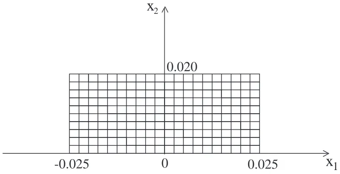
Assuming that the sample material was a carbon fiber reinforced plastic (CFRP), the conductivity _σc and the permeability _µ0 were taken as _σc = 1 ×106 [S/m] and _µ0 = 4_π×10−7 [H/m], respectively. In the numerical experiments, we assume that a single frequency was used, i. e.,, _M0 = 1 in (57). The alternating current _Js and the applied frequency _f = _ω/2_π were respectively given by _Js = 40 [mA] and _f = 100[_Hz]. The number of observation points was set as _m = 30 and the set of scanning positions of SQUID coil probe given by (14) were chosen as

¯

0

0.025

-0.025

x

x

0.020

Figure 10: The decomposition of sample material

where

oi = 0.0125 + 0.025i, i= 1,2,· · ·,30,

and where denotes a sufficiently small positive value to restrict the effective area of the SQUID pick-up coil. The scanning line in Fig. 9 were set as _r = 0_.0375[_m] and hf = 0.003[m], respectively.

To discretize the system model by a finite-element method, the reference domain G0∪G˜1s∪G˜2s was divided into a finite number of elements{ek}Kk=1e and a numberNe(> Ke)

of nodes defined by{x˜_i = (˜_xi_{1, x}˜i₂)}N_i=1e were selected in the reference domain. Each element is preassigned as an axiprallel rectangle with nodes at the vertices (see e. g., [13]). The number of finite elements and nodes in the numerical experiments reported in the sequel were set as_Ke= 3000(= 50×60) and_Ne = 3061(= 51×61) respectively. Figure 10 depicts the decomposition of the conducting material treated here. The number of elements and nodes in the material were taken as 200(= 10×20) and 231(= 11×21), respectively. Integration in the element matrices_KN(q) and the element vector _fN(q) were computed numerically by a Gauss-Legendre formula.

For these test example computations, simulated data {_zd} were generated by first solving the finite-Galerkin model (61) and (62). A series of random Gaussian noise were added to the numerical solutions, thereby producing simulated noisy data for the algo-rithm. The essential difficulties in (ASIDP)N _{come from the fact that real data are}

heavily corrupted by observation noise and it often occurs that the corresponding model output data are far from those practical data. Tikhonov regularization is one possible technique for avoiding these serious difficulties in computational efforts. To this end, we adopt Tikhonov’s regularization techniques to our inverse algorithm. More precisely, a regularization term is added to the cost functional (63) (see [14] for more details):

F_ηN(q) =_FN(q) + η 2

where

[L_c]_i,j =         

1 −1 0 · · · · 0 0 1 −1 0 · · · 0

..

. 0 . . . ... ... ..

. ... . .. ... 0 0 0 · · · 0 1 −1

        

∈ R(M−1)×M

In order to select the “optimal” parameter _η, we used L-curve analysis (see [15, 16]). The outline of this approach in these experiments is summarized as follows:

[L-curve analysis] : Given _η∈[0_,∞), solve F_ηN(ˆq(_η)) = min

q F N

η (q), (65)

for each fixed _η∈[0_,∞), collect the points _z˜N_(ˆq

η;ω)−zd(ω)

2

,L_cˆq_η2 (66)

and plot the above points. Then the ”optimal” parameter _η0 can be chosen as a point that lies in the ”corner” of the resulting curve.

Evaluation of the vector gradient of the cost function (65) is the computationally expensive part of our algorithm. This can be accomplished by using a co-state approach. For the numerical results reported in this paper, we used the gradient projection method ([17]) which is a particularly useful technique for optimization problems with linear inequality constraints such as those in (60). The iterative algorithm for finding ˆqN _{in this experiment}

is the same as that in [5].

In our test examples, we considered corrosion shape identification for conducting mate-rial samples with corrosion-like damage (of varying corrosion shape) as depicted in Fig. 6. The parameter function (59) to be identified is a piecewise linear spline function. We denote the knot sequence for _r by

−0_.025 =_τ0M _{< τ1}M _<· · · _{< τM}M₊₁ = 0_.025 and the unknown parameter vector qM _={qM

i }Mi=1 is then given by q_iM =_r(_τiM) for _i= 1_,2_,· · ·_{, M.}

For the computational experiments, the dimensions of unknown parameter vector qwas taken as _M = 19. The lower bound in (60) was chosen as _β = 0_.001. The initial guesses for the parameters were given by

q_iM =_h0(= 0_.02) (_i= 1_,2_,· · ·_{, M})

0 0.005

0.01 0.015 0.02 0.025

-0.02 -0.01 0 0.01 0.02

x [m]

x [m] Initial Guess

True function

1

2

Figure 11: True function and estimated function in Example 1 (noise free)

Example 1: In this test example, we deal with the shape recovery for the CFRP sam-ple with a symmetric type of corrosion as shown in Figure 11. The values of the true parameters were given by

q₁19=_q19₁₉ = 0_.0195 _q219 =_q1819= 0_.0190 _q319=_q1719= 0_.0185 _q419=_q19₁₆ = 0_.0180 q519=q1915 = 0.0175 q619 =q1419= 0.0170 q719=q1319= 0.0165 q819=q1912 = 0.0160

q199 =q1119= 0.0155 q1019= 0.0150.

The estimated parameters are listed in Table 1 using data that is with noise free, and with data containing 5%, 10%,and 20% relative noise. Fig. 12 depicts the L-curve for 5% noise case and _ηo = 5_.0×10−12 was chosen as the optimal regularization parameter in (64). The successful results is demonstrated in Fig. 13 that depicts the estimated shape using Tikhonov regularization with the optimal selection _ηo _{and without the regularization.}

Example 2: In this example, we deal with a somewhat more difficult case as compared to that of Example-1. The type of damage was given by a non-symmetric function as illustrated in Figure 14. We set the same dimension for the unknown parameter vector as in Example 1 and we also used the same knot sequence. The values of the true parameters were preassigned in

q119= 0.0195 q219= 0.0190 q319= 0.0185 q194 = 0.0180 q519 = 0.0175