Assessing the accuracy of loss estimation methods for supercapacitor energy storage devices operating under constant power cycling

Equatio n C hapter 1 Section 1

Assessing the Accuracy of Loss Estimation Methods for Supercapacitor

Energy Storage Devices Operating under Constant Power Cycling

Ponggorn Kulsangcharoen

1

, Christian Klumpner

1

, Mohamed Rashed

1

, Greg Asher

1

George Z. Chen

2

and Stuart A. Norman

3

1

_{Department of Electrical and Electronic Engineering}

2

_{Department of Chemical and Environmental Engineering}

Faculty of Engineering, University of Nottingham

University Park, Nottingham, NG7 2RD, UK

3

_{E.ON Technologies Limited, E.ON Technology Centre}

Ratcliffe on Soar, Nottingham, NG11 0EE, UK

Tel.: +44(0)115 846 6118

Fax.: +44(0)115 951 5616

Email:

[email protected]

URL:

http://www.nottingham.ac.uk/eee/

Acknowledgements

The project this report is based on was funded by E.ON as part of the E.ON International Research Initiative. Responsibility for the content of this publication lies with the author.

Keywords

«Efficiency», «Energy storage», «Estimation technique», «Power cycling», «Supercapacitors»

Abstract

This paper assesses different energy loss estimation methods using the supercapacitor model parameters extracted from the electrochemical impedance spectroscopy (EIS). Two energy loss estimation methods are applied to two similar supercapacitors from different manufacturers operating under constant power charge-discharge cycling. The simpler loss method uses only the impedance data that corresponds to the cycle frequency and the instantaneous current data whilst the more complex method uses the detailed impedance vs frequency dependency and the corresponding current harmonics available from the FFT. The experimental loss data (the benchmark) uses integration of instantaneous power processed by the supercapacitor. By comparing the difference between the estimated and the experimental losses, the performance of each method is assessed and the factors that influence the accuracy of the two loss estimation methods as well as their limitations are highlighted.

Introduction

(i.e. changes in impedance with temperature or bias voltage) may have a positive effect (when it reduces) on the losses of a given SC technology/manufacturer but may have a negative effect (when it increases) on another since each manufacturer uses different device structures/electrolyte/electrode materials. Therefore, it is important to perform a full SC characterization under various/relevant testing conditions to ensure that the SC efficiency can be maximized before they are deployed in a given application as part of an energy storage system (e.g. hybrid vehicle).

In the research literature, there are two common approaches used in SC characterization, which are small-signal and large-signal. For the small-signal approach, the SC impedance versus frequency is first determined using the electrochemical impedance spectroscopy technique. Then the SC impedance information can be used to determine the SC detailed equivalent models [1,6] and/or used directly to estimate SC power loss and efficiency [3,7,8]. For the large-signal approach, high current/power is applied to SCs directly in charge-discharge cycling pattern [6] and by calculating the SC in&out energy over a single charge-discharge cycle, SC efficiency and energy loss can be determined. To validate a given SC model, two independent approaches are usually employed and their results are cross evaluated for consistency. In [7,8], the SC efficiency and energy loss is estimated from the SC voltage obtained during the charge-discharge cycling test and the SC impedance from the EIS test. However, this method cannot determine SC energy loss precisely (>10-20% overestimate) since its formula is limited to use of a single set of RC parameter that correspond to the frequency of the charge-discharge cycling period. In addition, the minimum/maximum voltages across the bulk capacitance that correspond to the end/beginning of SC charge-discharge cycling used in the formula cannot be measured directly since they are subjected to voltage drop due to the series resistance. In [3], the SC efficiency and energy loss is estimated from the SC current during the charge/discharge tests and the SC high-order equivalent model obtained from the SC impedance modeling process. The errors that appear are due to the curve fitting algorithm required in the modeling process and the error due to the impedance versus frequency measurement and interpolation. Since a typical application requires the SC to charge-discharge over a relatively fixed duration of tens of seconds, the order of the SC model can be reduced to account for the relevant frequency range of the SC impedance, therefore the fitting algorithm can be simplified with reduced loss of accuracy. The simplified SC RC model is preferred in [6], which uses this approach to calculate an equivalent resistance that is highly dependent on the harmonic content of the SC current and the frequency and therefore cannot be used for generalized load conditions. The variation of the SC resistance with bias voltage was not considered.

In this paper, two SC current-based loss estimation techniques are evaluated. First, the SC characteristics of two devices similar in performance but from different manufacturers are determined using the electrochemical impedance spectroscopy (EIS). The two devices are then subjected to a charge-discharge constant power cycling (CPC) test but the result related to the accuracy of the estimated losses are inconclusive. A second set of tests is conducted, subjecting the device to pulse like stresses, which are more likely to mirror stresses from real applications. The more elaborate loss estimation technique is now proving more accurate. The SCs used in this evaluation are the Maxwell®

BCAP100 100F 2.7V that will be referred as M-SC and the Ioxus® _{RSC2R7107SR 100F 2.7V SC,}

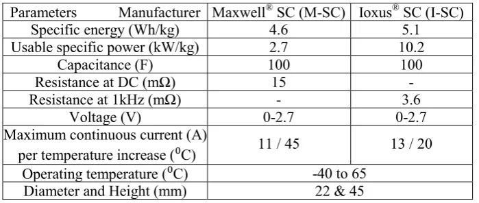
[image:2.595.124.474.619.767.2]

which will be referred as I-SC. Their specifications are shown in Table I.

Table I Specifications of the supercapacitor devices under test

Parameters Manufacturer Maxwell®SC (M-SC) Ioxus®SC (I-SC) Specific energy (Wh/kg) 4.6 5.1 Usable specific power (kW/kg) 2.7 10.2

Capacitance (F) 100 100

Resistance at DC (mΩ) 15 - Resistance at 1kHz (mΩ) - 3.6

Voltage (V) 0-2.7 0-2.7

Maximum continuous current (A)

per temperature increase (⁰C) 11 / 45 13 / 20 Operating temperature (⁰C) -40 to 65

Device Characterization using the electrochemical impedance spectroscopy

(EIS) method

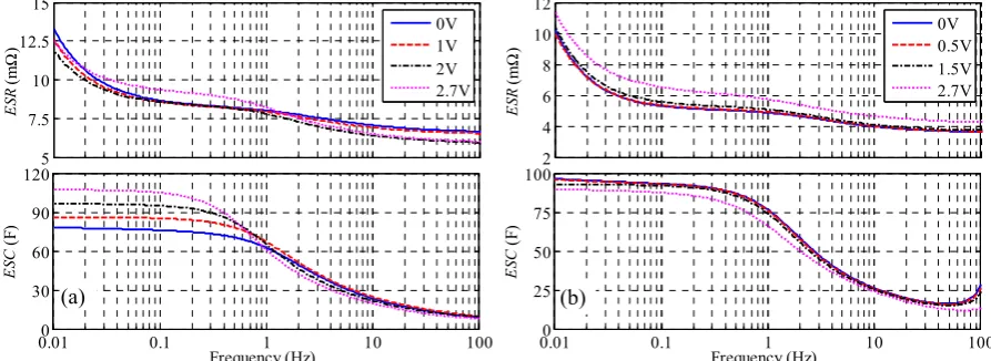
The EIS method applies a very small sinusoidal voltage signal to a single SC cell (e.g. 10 mV) and the current response signal is recorded. Both the voltage and the current information are used to extract the SC impedance change over a range of testing frequencies. The technique is very useful as it can be applied at various fixed bias voltage levels and at various fixed-temperature conditions [1,2]. From the SC impedance-frequency profiles, the SC equivalent models can be derived, which can be used to estimate efficiency and energy loss in corresponding to any given current and power profiles [3]. In this work, the Bio-logic SP-150 Potentiostat/Galvanostat machine equipped with a 20A current booster is used to perform the EIS tests, which has an impedance accuracy of <1% as stated in its specification. The EIS method is applied to M-SC and I-SC at various bias voltage and temperature conditions. The impedance results of both SCs are represented by using a single series-connected RC model are shown in Fig. 1 and Fig. 2 where ESR is the equivalent series resistance and ESC is the equivalent series capacitance.

Fig. 1(a) shows that as the bias voltage increases from 0V to 2.7V, the M-SC ESR@10mHz decreases from 13.3mΩ to 12.5mΩ (-6.2%) and its ESC@10mHz increases from 78F to 107F (+31%). When compared to the 0V bias parameters, these variations mean that as the device charges, the power circulation causes less loss due to lower ESR and also the capability of the device to store energy increases due to higher ESC. At 2V bias, as frequency increases from 10mHz to 100mHz, the ESR

reduces to 72.5% (11.9mΩ@10mHz/8.6mΩ@100mHz). On the other hand, from Fig. 1(b) shows that as the bias voltage increases from 0V to 2.7V, the I-SC ESR@10mHz increases from 10mΩ to 11mΩ

(+10%) and its ESC@10mHz decreases from 96F to 89F (-7.5%). At 1.5V bias, as frequency increases from 10mHz to 100mHz, the ESR reduces to 54% (10.4mΩ@10mHz/5.6mΩ@100mHz).

[image:3.595.72.519.557.720.2]

The implications of the variable parameters with bias voltage are opposite for the I-SC compared to M-SC. Also, the variation of parameters with frequency, although in the same direction, has different ratios for the I-SC compared to M-SC. But it can be generalized that for real industrial applications with charge-discharge cycles that exceed tens of seconds (frequency range is 10-100mHz), the wide variation of the ESR with frequency and also its opposite variation with bias voltage may result in significant errors (>20%) in the estimation of power losses for a particular working cycle and if a reasonable accuracy is required in the design stage, a more advanced methodology to enable the decrease of power loss errors below 5% is required. As frequency increases beyond _≈1Hz, the bias voltage affects both SC ESRs differently. From Fig. 1(a) and 1(b), M-SC ESR@100Hz decreases as the bias increases, whilst for I-SC, the bias voltage affects its ESR for across the entire frequency range. Even though both SCs are classified as supercapacitor-type energy storage with similar specifications (100F 2.7V), their parameter variation with the bias voltage are different.

Fig. 1: ESR and ESC versus frequency at various applied bias voltage and room temperature (25°C) of (a) M-SC (b) I-SC

5 7.5 10 12.5 15

ES

R

(m

Ω

)

0V 1V 2V 2.7V

0.010 0.1 1 10 100

30 60 90 120

ES

C

(F

)

Frequency (Hz)

2 4 6 8 10 12

ES

R

(m

Ω

)

0V 0.5V 1.5V 2.7V

0.010 0.1 1 10 100

25 50 75 100

ES

C(F

)

Frequency (Hz)

[image:4.595.72.520.173.338.2]

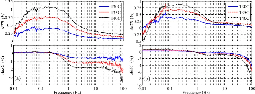
From Fig. 2(a) and 2(b), the effect of the operating temperature increase from 25°C to 40°C on both M-SC and I-SC ESRs reduction, ΔESR, are ≈1% maximum across the entire frequency range. The effect of temperature change on both SC ESCs is also small (<1%) for the frequency less than _≈1Hz. As the frequency increases beyond 1Hz, M-SC and I-SC ESC reductions, ΔESC, are 4% and 9% maximum. The ESR and ESC information collected via EIS at ambient temperature and at a bias voltage similar to the average cycle test voltage will be used in the SC loss estimation algorithms where the devices under test will be subject to constant power cycling.

Fig. 2: Change in ESR and ESC versus frequency at 2V constant bias voltage under various temperatures in comparison with room temperature (25°C) of (a) M-SC (b) I-SC

Estimating the power losses under constant power cycling method based on

SC voltage and current measurements

The constant power cycling (CPC) method is originally used in aging tests [4,5,8,9] to study SC degradation. The authors have adopted this method for evaluating the SC round-trip efficiency and loss [8] based on direct measurement of SC power in and power out, allowing the direct measurement of energies in and out and direct calculation of the energy loss over a cycle. This is why the results based on this method will be referred as experimental (EXP). To control the SC power constantly,

pSC_Ref, a current reference, iSC_Ref, is adjusted according to the SC stack voltage, vSC, change by iSC_Ref

=pSC_Ref/vSC. The vSC is also monitored and used for toggling the current direction as well as the power

direction when the preset SC min/max voltage thresholds are reached. Thus, the round-trip efficiency,

ηRT, and energy loss, ELossRT_EXP, of SCs can be determined by performing integration on a single

charge-discharge cycle of the SC power waveform as:

η = −

∫

D

∫

C = − = −

T T

RT SC SC D D C C D C

0 0

p dt p dt P T P T E E (1)

= +

LossRT _ EXP C D

E E E (2)

= +

Cycle C D

T T T (3)

where pSC is the instantaneous power through the SC calculated from the product of current, iSC, and

voltage, vSC, PC and PD are the average charging and discharging power, EC and ED are the charging

and discharging energy, TC and TD are SC charging and discharging duration and TCycle is

charge-discharge period. In this paper, the CPC method is performed on single cells of M-SC and I-SC by using the Bio-logic Potentiostat/Galvanostat machine which has its technology based on a linear amplifier. Therefore, there is no switching ripple and other high-frequency harmonics present in SC current and voltage waveforms. The Bio-logic machine equipped with 20A Booster has 16-bit ADC, which gives voltage and current reading resolution as small as 50µV and 2mA which is very accurate.

There are two constant-power patterns applied to both SC devices, which are: continuous constant power cycling (CCPC); at power levels of 7W and 21W and pulse constant power cycling (PCPC) at a power level of 26W with a 30s relaxation time as shown in Fig. 3-5. Both tests are done with the same

0 0.25 0.5 0.75 1 1.25

Δ

ES

R

(%

)

T30C T35C T40C

0.01 0.1 1 10 100

-4 -3 -2 -1 0 1

Δ

ES

C

(%

)

Frequency (Hz)

-0.5 -0.25 0 0.25 0.5 0.75 1

Δ

ES

R

(%

)

T30C T35C T40C

0.01 0.1 1 10 100

-10 -8 -6 -4 -2 0 2

Δ

ES

C (%

)

Frequency (Hz)

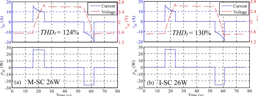
min/max vSC setting of 1.35V/2.7V which are the SC half- and the SC rated-voltages. The selection of

SC power and min/max vSC in the test is done such that the SC RMS current and the temperature rise is

less than the rated values shown in Table I. The total harmonic distortion, THDI, of the SC current is

also calculated for all experimental waveforms and included in the figures. The CCPC THDI is 56–

58% and the PCPC THDI is 124–130%, which is means significantly higher distortion than that of the

[image:5.595.74.519.172.338.2]

CCPC, and therefore a higher amount of loss expected to be caused by harmonic currents though the equivalent ESRs.

[image:5.595.73.516.368.537.2]

Fig. 3: The SC current, voltage and power during the 7W CCPC test of (a) M-SC and (b) I-SC

Fig. 4: The SC current, voltage and power during the 21W CCPC test of (a) M-SC and (b) I-SC

Fig. 5: The SC current, voltage and power during the 26W PCPC test of (a) M-SC and (b) I-SC

-6 -3 0 3 6 iSC (A ) 1.2 1.6 2 2.4 2.8 vSC (V ) Current Voltage

0 10 20 30 40 50 60 70 80

-8 -4 0 4 8 pSC (W ) Time (s) -6 -3 0 3 6 iSC (A ) 1.2 1.6 2 2.4 2.8 vSC (V ) Current Voltage

0 10 20 30 40 50 60 70

-8 -4 0 4 8 pSC (W ) Time (s) -20 -10 0 10 20 iSC (A ) 1.2 1.6 2 2.4 2.8 vSC (V ) Current Voltage

0 4 8 12 16 20 24

-30 -20 -10 0 10 20 30 pSC (W ) Time (s) -20 -10 0 10 20 iSC (A ) 1.2 1.6 2 2.4 2.8 vSC (V ) Current Voltage

0 3 6 9 12 15 18 21

-30 -20 -10 0 10 20 30 pSC (W ) Time (s) -20 -10 0 10 20 iSC (A ) 1.2 1.6 2 2.4 2.8 vSC (V ) Current Voltage

0 10 20 30 40 50 60 70 80

-30 -20 -10 0 10 20 30 pSC (W ) Time (s) -20 -10 0 10 20 iSC (A ) 1.2 1.6 2 2.4 2.8 vSC (V ) Current Voltage

0 10 20 30 40 50 60 70 80

-30 -20 -10 0 10 20 30 pSC (W ) Time (s)

(a)

M-SC 26W

THD

I

= 124%

(b)

I-SC 26W

THD

I

= 130%

(a)

M-SC 21W

THD

I

= 56%

(b)

I-SC 21W

THD

I

= 56%

(b)

I-SC 7W

THD

I

= 58%

(a)

THD

I

= 58%

[image:5.595.74.515.569.733.2]

The cycling test is performed continuously for one hour to let the SC device temperature, TempSC, to

reach steady-state as shown in the bottom figures of Fig. 6–8. Using (1)–(3), the ηRT, ELoss_RT_EXP and

TCycle of both SCs are calculated and plotted against the elapsed test time as shown in the same figures.

Fig. 6 shows that over the entire 7W CCPC test there is not a noticeable change in ηRT (≈96.15% for

M-SC and _≈96.75% for I-SC) and same applies for the ELossRT_EXP (≈10.15J for M-SC and ≈7.2J for

I-SC) since the ESR reduction effect due TempSC increases is small (only 3–4°C increase). In Fig. 7, the

processing power is changed to 21W, so more energy loss is produced contributing to a higher TempSC

increase (≈10°C in addition to room temperature) which causes a noticeable reduction in ESR. The ηRT

of both devices are increased by a noticeable amount of 0.3–0.4% (91.15%→91.45% for M-SC and 93.4%→93.75% for I-SC) and their ELossRT_EXP values are reduced by 0.5–0.7J (21.3J→20.8J for M-SC

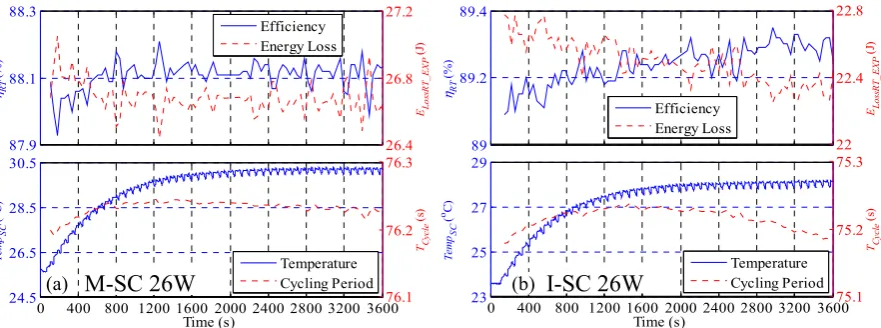
and 14.4J→13.7J for I-SC). In Fig. 8, a 26W pulsed constant power cycling (PCPC) charge-discharge pattern with a 30s relaxation time is applied to the two SC under test. Even though the applied power level is higher than the 21W CCPC, the TempSC rise over the cycling test is small due to the long

relaxation, which gives average cycle losses and temperature increase similar to the 7W CCPC condition (5°C). However, there is only a 0.2% improvement in both device ηRT (87.9%→88.1% for

M-SC and 89.1%→89.3% for I-SC) due to ESR decrease and correspondingly an ELossRT_EXP reduction

[image:6.595.77.524.299.458.2]

by 0.2–0.4J (26.8J→26.6J for M-SC and 22.8J→22.4J for I-SC).

[image:6.595.76.522.504.667.2]

Fig. 6: The SC round-trip efficiency, energy loss over a cycle, temperature and charge-discharge cycle period during the 7W CCPC test of (a) M-SC and (b) I-SC

Fig. 7: The SC round-trip efficiency, energy loss over a cycle, temperature and charge-discharge cycle period during the 21W CCPC test of (a) M-SC and (b) I-SC

96.1 96.2 96.3 ηRT (% ) 10.05 10.15 10.25 EL os sRT _ EXP (J ) Efficiency Energy Loss

0 400 800 1200 1600 2000 2400 2800 3200 3600 23 24 25 26 Te m pSC ( oC) Time (s) 74.2 74.3 TC ycl e (s ) Temperature Cycling Period 96 96.5 97 ηRT (% ) 7.1 7.35 7.6 EL os sRT _ EXP (J ) Efficiency Energy Loss

0 400 800 1200 1600 2000 2400 2800 3200 3600

24 25 26 27 Te m pSC ( oC) Time (s) 64.5 64.6 64.7 64.8 TC ycl e (s ) Temperature Cycling Period 91.1 91.3 91.5 ηRT (% ) 20.6 21.1 21.6 ELo ss RT _ EXP (J ) Efficiency Energy Loss

0 900 1800 2700 3600

26 29 32 35 38 Te mp SC ( oC) Time (s) 20.3 20.7 21.1 TC ycle (s ) Temperature Cycling Period 93.4 93.6 93.8 ηRT (% ) 13.5 14 14.5 ELo ssR T_ E X P (J ) Efficiency Energy Loss

0 400 800 1200 1600 2000 2400 2800 3200 3600 23 26.5 30 33.5 37 Te m pSC ( oC) Time (s) 20.2 20.5 TC ycle (s ) Temperature Cycling Period

(a) (b)

M-SC 21W

I-SC 21W

[image:7.595.79.520.74.238.2]

Fig. 8: The round-trip efficiency, loss, temperature and charge-discharge period during the 26W PCPC test of (a) M-SC and (b) I-SC

In bottom graphs of Fig. 6-8, it can be seen that as TempSC approaches its steady-state condition, TCycle

for both SC do not change significantly compared with their initial values (<1s change for all testing conditions) which means that the ESR change and the associated loss is not due to the period/frequency shift but due to the temperature change. The other parameter that would influence the period for a given load condition, the ESC, has been shown in Fig. 2 not to change in the frequency range 10-100mHz when TempSC increases by 10–15°C. Next, the SC energy loss estimation methods

which use the iSC data obtained from the CPC tests presented in this section will be discussed.

Energy loss estimation based on SC current and EIS equivalent parameters

Energy loss estimation using the time domain SC current (RMS method)

To estimate energy loss during the CPC test, the SC root-mean-square current, ISC_RMS, is calculated

from iSC(t) over a single charge-discharge cycling period, TCycle. Using this RMS current in Joules loss

formula (I2_{R), the RMS-based SC energy loss over the cycle, E}

LossEST_RMS is:

(

)

= 2

LossEST _ RMS SC _ RMS Cycle Cycle

E I ESR T (4)

where ESRCycle is the actual SC ESR reading from the EIS result at the exact frequency corresponding

to TCycle. In (4), only one ESR is used from the EIS result for the estimation, which makes this

estimation technique very simple to implement. However, at very low cycle frequencies (<<0.1Hz), there are two mechanisms that can cause significant errors in the estimation of losses: first, the ESR that is used in conjunction with the harmonic currents is constant in (4) but in reality, it decreases significantly with the harmonic order, which would lead to overestimating the losses; secondly, very low frequencies that have a very long corresponding cycle duration are typically performed at reduced power/current which means that losses associated with the SC self-discharge current, which are omitted in (4), will cause a significant underestimation of losses. These two mechanisms may have a tendency to cancel each other, especially when the harmonic content is reduced (low THD). This was the reason why the two types of power cycling discussed before were chosen to assess the accuracy of the two estimation methods. To make full use of the available SC impedance information, iSC is

converted to the frequency domain in the next section.

Energy loss estimation using the frequency domain SC current (FFT method)

This estimation method uses the Fast Fourier Transform algorithm (FFT) to convert the iSC signal

obtained during the CPC test in order to analyze them in the frequency domain. By applying the FFT, the fundamental, the harmonics and the DC components of the SC currents are extracted. Using the SC current fundamental and harmonic parts, Ik, with the ESRk at the corresponding frequency from the EIS

results, a power loss, PEST_k of each kth frequency component can be calculated. Accumulating this

power loss up to the highest relevant frequency order, M, and combining it with the power loss caused by the DC current component, IDC, and the average bias voltage, VBias, the total power loss is obtained.

The estimated cycle energy loss, ELossEST_FFTis found by multiplying the total power loss with TCycle:

87.9 88.1 88.3

ηRT

(%

)

26.4 26.8 27.2

ELo

ss

R

T

_E

X

P

(J

)

Efficiency Energy Loss

0 400 800 1200 1600 2000 2400 2800 3200 3600 24.5

26.5 28.5 30.5

Te

m

pSC

(

oC)

Time (s)

76.1 76.2 76.3

TC

ycle

(s

)

Temperature Cycling Period

89 89.2 89.4

ηRT

(%

)

22 22.4 22.8

EL

os

sRT

_

EXP

(J

)

Efficiency Energy Loss

0 400 800 1200 1600 2000 2400 2800 3200 3600 23

25 27 29

Te

mp

SC

(

oC)

Time (s)

75.1 75.2 75.3

TC

ycl

e

(s

)

Temperature Cycling Period

(

)

= ⎛ ⎞ =⎜ + ⎟ ⎝

∑

⎠ M

LossEST _ FFT EST _ k DC Bias Cycle k 1

E P I V T (5)

= 2

EST _ k k k

P I ESR (6)

By performing the loss estimation in the frequency domain, the effect of the error due to using a single impedance measurement point from the EIS test is minimised as more ESR measurement points at the relevant frequencies are used. However, the limitation of this approach is that a very detailed EIS profile is needed to improve the accuracy of the loss estimation. There may still be errors in the method: first, the DC current component is typically very low and influenced by the error of the data acquisition system; secondly, the average bias voltage may need to consider the variation profile and not be just an arithmetic average of the cycle minimum and maximum voltage; thirdly, in order to save time on the EIS characterization, a finite number of EIS data points is measured and linear interpolation is used to derive ESRk where exact measured data points are not available.

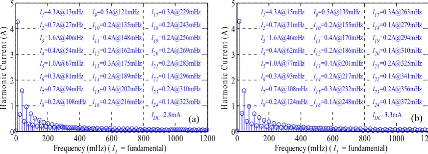
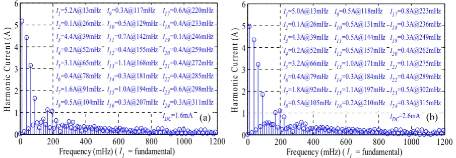
The FFT method is applied to the M-SC and I-SC currents shown in Fig. 3-5, which produce the corresponding current harmonic spectrums as shown in Fig. 9–11. It can be seen that the harmonic current patterns of the CCPC test has very large fundamental component compared with the other harmonics, which means that the RMS of the total SC current (and its corresponding loss) is mainly determined by the fundamental component. On the other hand, the harmonic current patterns of the PCPC test is quite different from that of the CCPC test as the 3rd_{, 5}th_{, 7}th _{etc harmonics become}

significantly larger in amplitude which will affect the total RMS value. It can be noted that the high order current harmonics (>20th _{order) are very low and as their corresponding ESR further decreases, it}

[image:8.595.76.513.395.552.2]

means that they would have insignificant contribution to the overall losses. However, in order to achieve highest precision when comparing the two loss estimation methods, all harmonic currents shown in Fig. 9-11 are included in the loss calculation.

[image:8.595.76.521.582.743.2]

Fig. 9: The SC current harmonics during the 7W CCPC test of (a) M-SC and (b) I-SC

Fig. 10: The SC current harmonics during the 21W CCPC test of (a) M-SC and (b) I-SC

0 200 400 600 800 1000 1200

0 1 2 3 4 5

I₁=4.3A@13mHz

I₂=0.7A@27mHz

I₃=1.6A@40mHz

I₄=0.4A@54mHz

I₅=1.0A@67mHz

I₆=0.3A@81mHz

I₇=0.7A@94mHz

I₈=0.2A@108mHz

I₉=0.5A@121mHz

I₁₀=0.2A@135mHz

I₁₁=0.4A@148mHz

I₁₂=0.2A@162mHz

I₁₃=0.3A@175mHz

I₁₄=0.2A@189mHz

I₁₅=0.3A@202mHz

I₁₆=0.2A@216mHz

I₁₇=0.3A@229mHz

I₁₈=0.2A@243mHz

I₁₉=0.2A@256mHz

I₂₀=0.2A@269mHz

I₂₁=0.2A@283mHz

I₂₂=0.1A@296mHz

I₂₃=0.2A@310mHz

I₂₄=0.1A@323mHz

I_DC=2.8mA

H ar m on ic Cu rr en t ( A )

Frequency (mHz) ( I₁ = fundamental) 0 200 400 600 800 1000 1200 0 1 2 3 4 5

I₁=4.3A@15mHz

I₂=0.7A@31mHz

I₃=1.6A@46mHz

I₄=0.4A@62mHz

I₅=1.0A@77mHz

I₆=0.3A@93mHz

I₇=0.7A@108mHz

I₈=0.2A@124mHz

I₉=0.5A@139mHz

I₁₀=0.2A@155mHz

I₁₁=0.4A@170mHz

I₁₂=0.2A@186mHz

I₁₃=0.4A@201mHz

I₁₄=0.2A@217mHz

I₁₅=0.3A@232mHz

I₁₆=0.1A@248mHz

I₁₇=0.3A@263mHz

I₁₈=0.1A@279mHz

I₁₉=0.2A@294mHz

I₂₀=0.1A@310mHz

I₂₁=0.2A@325mHz

I₂₂=0.1A@341mHz

I₂₃=0.2A@356mHz

I₂₄=0.1A@372mHz

I_DC=3.3mA

H ar m on ic Cu rr en t ( A )

Frequency (mHz) ( I₁ = fundamental)

0 500 1000 1500 2000 2500 3000 3500 4000 4500

0 2 4 6 8 10 12 14

I₁=12.7A@45mHz

I₂=2.0A@90mHz

I₃=4.5A@135mHz

I₄=1.4A@180mHz

I₅=2.7A@225mHz

I₆=1.2A@270mHz

I₇=1.8A@315mHz

I₈=1.0A@360mHz

I₉=1.3A@406mHz

I₁₀=1.0A@451mHz

I₁₁=0.9A@496mHz

I₁₂=0.9A@541mHz

I₁₃=0.7A@586mHz

I₁₄=0.9A@631mHz

I₁₅=0.5A@676mHz

I₁₆=0.8A@721mHz

I₁₇=0.4A@766mHz

I₁₈=0.7A@811mHz

I₁₉=0.3A@856mHz

I₂₀=0.7A@901mHz

I₂₁=0.2A@946mHz

I₂₂=0.6A@991mHz

I₂₃=0.2A@1036mHz

I₂₄=0.6A@1081mHz

I_DC=3.7mA

H arm on ic C urre nt (A )

Frequency (mHz) ( I₁ = fundamental) 0 500 1000 1500 2000 2500 3000 3500 4000 4500

0 2 4 6 8 10 12 14

I₁=12.8A@49mHz

I₂=2.0A@98mHz

I₃=4.7A@147mHz

I₄=1.2A@196mHz

I₅=2.8A@245mHz

I₆=1.0A@295mHz

I₇=1.9A@344mHz

I₈=0.9A@393mHz

I₉=1.4A@442mHz

I₁₀=0.8A@491mHz

I₁₁=1.1A@540mHz

I₁₂=0.7A@589mHz

I₁₃=0.9A@638mHz

I₁₄=0.7A@687mHz

I₁₅=0.7A@736mHz

I₁₆=0.7A@785mHz

I₁₇=0.6A@835mHz

I₁₈=0.6A@884mHz

I₁₉=0.5A@933mHz

I₂₀=0.6A@982mHz

I₂₁=0.4A@1031mHz

I₂₂=0.6A@1080mHz

I₂₃=0.3A@1129mHz

I₂₄=0.5A@1178mHz

I_DC=4.1mA

Har m on ic Cu rr en t ( A )

Frequency (mHz) ( I₁ = fundamental)

(a) (b)

[image:9.595.72.525.76.233.2]

Fig. 11: The SC current harmonics during the 26W PCPC test of (a) M-SC and (b) I-SC

Comparison of energy loss estimation

The SC cycling energy loss determined from V&I (power) data referred to as EXP (experimental) and the two SC current based methods are applied to both devices under test during the previous tests: the 7W CCPC (Fig. 3), the 21W CCPC (Fig. 4) and the 26W PCPC (Fig. 5). The evaluation of the losses determined with the three methods and their relative percentage difference against the power based method (EXP) are shown in Fig. 12-

Fig. 14

. The power based method (EXP) is considered the benchmark because its error is only affected by the voltage and current measurement errors which can be minimized by the high accuracy of the impedance spectroscopy machine. It can be seen that the difference between the estimated loss of the SC current based methods and the power based method is typically not higher than 5%.

During the low power (7W) CCPC test shown in Fig. 12, it can be noticed that the RMS method produces more accurate result than the FFT method and the reason is that for this particular condition, the two opposite error mechanisms that cause underestimation (ESR of fundamental cycle frequency considered for high order current harmonic) and overestimation (omission of loss due to the DC current component) are cancelling out. This is not the case in the high power (21W) CCPC test shown in Fig. 13 where the RMS method gives highest errors. It can be seen that at the beginning of the test when the device temperature is closest to the room temperature/EIS test condition, the absolute cycle energy loss error (in J) between the FFT method and the power based (EXP) method stays constant for both devices under test at about 0.15-0.2J for both power levels. As time passes, the high power test causes warming of the device and this explains the larger drift in the estimated loss (error reaches 0.5-0.7J), smaller for I-SC as its impedance variation is more immune to temperature variations.

In contrary, the discrepancy between the cycle energy loss of the RMS method and the benchmark seems to vary quite a lot from less than 0.05J for the I-SC at low power to almost 1J for both devices at high power. There is an additional reason why the error during the high power CCPC test increases with time, which is the change of ESR with temperature that is not considered in the two SC current based methods. The reduction in ESR is real and this is shown by the decrease of losses from 21.2J at the start of the test to 20.8J after 2000 seconds (Fig. 13a). Further improvement of both loss estimation techniques can be possible by integrating a mechanism to account for the device parameter change with temperature, which can be directly measured or estimated.

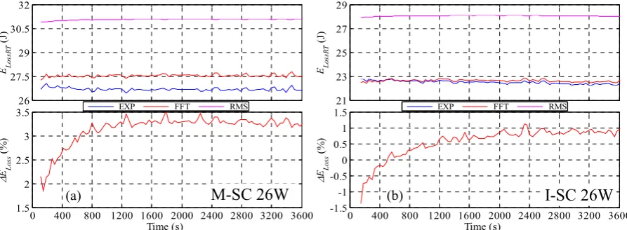
The previous CCPC tests resulted in a current waveform which was very similar to a square wave, being characterized by a fairly low THD which resulted in small differences in precision between the two estimation methods. A third test that would result in highly distorted current shapes that would cause higher losses due to the higher current harmonics (Fig. 11) was conducted and the results are shown in Fig. 14. The power pulse is 26W which is similar to the high power CCPC test. It can be seen that the loss estimation using the RMS method shows significant differences compared to the power based (EXP) method: 15% for M-SC and 28% for I-SC. Fig. 14-bottom shows that the differences of the FFT method remain below 2% at the beginning of the test (M-SC device at room

0 200 400 600 800 1000 1200

0 1 2 3 4 5 6

I₁=5.2A@13mHz

I₂=0.1A@26mHz

I₃=4.4A@39mHz

I₄=0.2A@52mHz

I₅=3.1A@65mHz

I₆=0.4A@78mHz

I₇=1.6A@91mHz

I₈=0.5A@104mHz

I₉=0.3A@117mHz

I₁₀=0.5A@129mHz

I₁₁=0.7A@142mHz

I₁₂=0.4A@155mHz

I₁₃=1.1A@168mHz

I₁₄=0.3A@181mHz

I₁₅=1.0A@194mHz

I₁₆=0.3A@207mHz

I₁₇=0.6A@220mHz

I₁₈=0.4A@233mHz

I₁₉=0.1A@246mHz

I₂₀=0.4A@259mHz

I₂₁=0.4A@272mHz

I₂₂=0.4A@285mHz

I₂₃=0.6A@298mHz

I₂₄=0.3A@311mHz

I_DC=1.6mA

H

ar

m

on

ic

C

urr

en

t (A

)

Frequency (mHz) ( I₁ = fundamental) 0 200 400 600 800 1000 1200 0

1 2 3 4 5 6

I₁=5.0A@13mHz

I₂=0.1A@26mHz

I₃=4.3A@39mHz

I₄=0.2A@52mHz

I₅=3.2A@66mHz

I₆=0.4A@79mHz

I₇=1.8A@92mHz

I₈=0.5A@105mHz

I₉=0.5A@118mHz

I₁₀=0.5A@131mHz

I₁₁=0.5A@144mHz

I₁₂=0.5A@157mHz

I₁₃=1.0A@171mHz

I₁₄=0.3A@184mHz

I₁₅=1.1A@197mHz

I₁₆=0.2A@210mHz

I₁₇=0.8A@223mHz

I₁₈=0.3A@236mHz

I₁₉=0.3A@249mHz

I₂₀=0.4A@262mHz

I₂₁=0.1A@275mHz

I₂₂=0.4A@289mHz

I₂₃=0.5A@302mHz

I₂₄=0.3A@315mHz

I_DC=2.6mA

H

arm

on

ic

C

urre

nt

(A

)

Frequency (mHz) ( I₁ = fundamental)

[image:10.595.72.519.117.280.2]

temperature) and not exceeding 3.5% whilst the precision of the I-SC device remains between -/+ 1%. The differences in losses are smaller than at high power CCPC because the pulsed nature of the test causes lower average losses per cycle and therefore errors due to the impedance drift are lower.

[image:10.595.73.521.320.491.2]

Fig. 12: The three estimated cycle energy loss and the discrepancies of the SC current based vs the power based method during the 7W CCPC test of (a) M-SC and (b) I-SC

Fig. 13: The three estimated cycle energy loss and the discrepancies of the SC current based vs the power based method during the 21W CCPC test of (a) M-SC and (b) I-SC

Fig. 14: The three estimated cycle energy loss and the discrepancies of the SC current based vs the power based method during the 26W PCPC test of (a) M-SC and (b) I-SC

9.8 9.9 10 10.1 10.2

EL

ossR

T

(J

)

EXP FFT RMS

0 400 800 1200 1600 2000 2400 2800 3200 3600

-2.5 -2 -1.5 -1 -0.5 0

Δ

ELo

ss

(%

)

Time (s)

7 7.1 7.2 7.3 7.4 7.5

ELo

ss

R

T

(J

)

EXP FFT RMS

0 400 800 1200 1600 2000 2400 2800 3200 3600

-4 -3 -2 -1 0 1 2

Δ

ELo

ss

(%

)

Time (s)

20.5 21 21.5 22

ELo

ss

R

T

(J

)

EXP FFT RMS

0 400 800 1200 1600 2000 2400 2800 3200 3600

1 2 3 4 5 6

Δ

ELo

ss

(%

)

Time (s)

13.5 14 14.5

E Lo

ss

R

T

(J

)

EXP FFT RMS

0 400 800 1200 1600 2000 2400 2800 3200 3600

-2 0 2 4 6

Δ

E Lo

ss

(%

)

Time (s)

26 27.5 29 30.5 32

ELo

ss

R

T

(J

)

EXP FFT RMS

0 400 800 1200 1600 2000 2400 2800 3200 3600

1.5 2 2.5 3 3.5

Δ

ELo

ss

(%

)

Time (s)

21 23 25 27 29

E Lo

ss

R

T

(J

)

EXP FFT RMS

0 400 800 1200 1600 2000 2400 2800 3200 3600

-1.5 -1 -0.5 0 0.5 1 1.5

Δ

E Lo

ss

(%

)

Time (s)

(a)

M-SC 26W

(b)

I-SC 26W

(a)

M-SC 21W

(b)

I-SC 21W

[image:10.595.73.520.533.697.2]

Conclusion

Supercapacitos are typically used in power intense applications which means they are subject to significant stresses that could contribute to aging and device parameter variation. Being able to estimate accurately the losses in a device during the design stage is therefore important to ensure that early failure of SC in the equipment is avoided. To achieve that, it is therefore important to have available accurate tools to determine the losses in the device.

In this paper, two loss estimation methods based on the SC current and the SC impedance parameters were evaluated on two SCs from different manufacturers with similar specification (100F 2.7V). First a thorough evaluation of the devices under test was performed using the electrochemical impedance spectroscopy conducted at different bias voltages and temperature to identify which factors influence the variability of impedance data. Only the EIS data at ambient temperature and bias voltage similar to the average cycle test voltage were supplied to the loss estimation algorithms.

It can be concluded that the FFT current based method to estimate losses provides excellent precision in a wide range of SC powers and operating modes (continuous and pulsed power). The downside is that it relies on high computational power to perform the FFT and a very good knowledge of the device under test (very detailed EIS data).

The RMS method is much simpler to implement and may provide reasonable precision in estimating the losses for some particular operating conditions. However, the SC usually operates in conjunction to a power converter that causes a significant current ripple in the device. This will increase the total RMS current and therefore will cause an overestimation of SC losses. In reality, the switching ripple will be at high frequency where the ESR of the device is negligible, so the switching ripple will contribute very little to the SC losses, therefore, a method to remove the switching ripple from RMS calculation (e.g. low pass filter) is necessary.

References

[1] F. Rafik, H. Gualous, R. Gallay, A. Crausaz, and A. Berthon, "Frequency, thermal and voltage

supercapacitor characterization and modeling," J. Power Sources, vol. 165, pp. 928-934, 2007.

[2] M. Uno and K. Tanaka, "Accelerated Charge&Discharge Cycling Test and Cycle Life Prediction Model for

Supercapacitors in Alternative Battery Applications," IEEE Trans. Ind. Elec., vol. 59, pp. 4704-4712, 2012.

[3] T. Funaki, "Evaluating Energy Storage Efficiency by Modeling the Voltage and Temperature Dependency

in EDLC Electrical Characteristics," IEEE Trans. Power Elec., vol. 25, pp. 1231-1239, 2010.

[4] R. Chaari, O. Briat, J. Y. Delétage, E. Woirgard, and J. M. Vinassa, "How supercapacitors reach end of life

criteria during calendar life and power cycling tests," Microelec. Reliability, vol. 51, pp. 1976-1979, 2011.

[5] R. Chaari, O. Briat, J. Y. Deletage, and J. Vinassa, "Performances regeneration of supercapacitors during

accelerated ageing tests in power cycling," Proc. EPE 2011, Birmingham, UK, 2011, pp. 1-7.

[6] N. Rizoug, P. Bartholomeus, and P. Le Moigne, "Modeling and Characterizing Supercapacitors Using an

Online Method," IEEE Trans. Ind. Elec., vol. 57, pp. 3980-3990, 2010.

[7] M. W. Verbrugge and P. Liu, "Analytic solutions and experimental data for cyclic voltammetry and

constant-power operation of capacitors consistent with HEV applications," J. The Electrochem. Soc., vol.

153, pp. A1237-A1245, 2006.

[8] P. Kulsangcharoen, C. Klumpner, M. Rashed, and G. Asher, "A new duty cycle based efficiency estimation

method for a supercapacitor stack under constant power operation," Proc. PEMD2010, UK, 2010, pp. 1-6.

[9] K. Paul, M. Christian, V. Pascal, C. Guy, R. Gerard, and Z. Younes, "Constant power cycling for

accelerated ageing of supercapacitors," Proc. EPE2009, Barcelona, Spain, 2009, pp. 1-10.

[10] A. Hijazi, P. Kreczanik, E. Bideaux, P. Venet, G. Clerc, and M. Di Loreto, "Thermal Network Model of