Shadow Detection Method Based on HMRF with Soft Edges for High Resolution Remote Sensing Images

ISSN Online: 2159-4481 ISSN Print: 2159-4465

DOI: 10.4236/jsip.2019.104011 Nov. 29, 2019 200 Journal of Signal and Information Processing

Shadow Detection Method Based on HMRF with

Soft Edges for High-Resolution Remote-Sensing

Images

Wenying Ge

School of Computer and Information Engineering, Anyang Normal University, Anyang, China

Abstract

Shadow detection is a crucial task in high-resolution remote-sensing image processing. Various shadow detection methods have been explored during the last decades. These methods did improve the detection accuracy but are still not robust enough to get satisfactory results for failing to extract enough information from the original images. To take full advantage of various fea-tures of shadows, a new method combining edges information with the spec-tral and spatial information is proposed in this paper. As known, edge is one of the most important characteristics in the high-resolution remote-sensing images. Unfortunately, in shadow detection, it is a high-risk strategy to de-termine whether a pixel is the edge or not strictly because intensity values on shadow boundaries are always between those in shadow and non-shadow areas. Therefore, a soft edge description model is developed to describe the degree of each pixel belonging to the edges or not. Sequentially, the soft edge description is incorporating to a fuzzy clustering procedure based on HMRF (Hidden Markov Random Fields), in which more appropriate spatial contex-tual information can be used. More concretely, it consists of two components: the soft edge description model and an iterative shadow detection algorithm. Experiments on several remote sensing images have shown that the proposed method can obtain more accurate shadow detection results.

Keywords

Shadow Detection, Soft Edges, Clustering, Remote-Sensing Images

1. Introduction

Remote sensing images are applied in many fields, including geography map-ping, agriculture, change detection, etc. Unfortunately, shadows in these images How to cite this paper: Ge, W.Y. (2019)

Shadow Detection Method Based on HMRF with Soft Edges for High-Resolution Re-mote-Sensing Images. Journal of Signal and Information Processing, 10, 200-210.

https://doi.org/10.4236/jsip.2019.104011 Received: October 10, 2019

Accepted: November 26, 2019 Published: November 29, 2019 Copyright © 2019 by author(s) and Scientific Research Publishing Inc. This work is licensed under the Creative Commons Attribution International License (CC BY 4.0).

DOI: 10.4236/jsip.2019.104011 201 Journal of Signal and Information Processing obstruct these applications because of the reduction or even loss of radiance in the shadow areas. To detect shadows, early works extracted spectral features of shadow areas, such as lower intensity [1], higher saturation [2], large hue value and blow blue color value [3], etc. Later, in order to take full advantages of spec-tral features of multiband images, some researches explored invariant color spaces to stress the differences between shadows and non-shadows[4] [5] [6]. Also, some efforts on combining different spectral features [7] [8] have achieved some good results in their intended realms. However, there are still some limits in these methods because of the absence of other information such as edges and spatial context information.

As for spatial information, the well-known probabilistic model HMRF which serve as a powerful formal tool to present neighborhood interactions is a natural choice [9]. In recent years, many researchers have attempted to incorporate more information into it to improve the performance of HMRF [10] [11]. Our latest work [12] adds edge constraints into the iterative clustering procedure based on HMRF. In this work, an edges consistency model is proposed to de-scribe the similarity between the clustering edges and the pre-detected ones. This method can obtain more clear boundaries along with the homogeneous area. However, it is not a good idea to determine whether a pixel is the edge or not strictly because the spectral features of pixels on the shadow boundaries are not discriminable enough.

In this paper, a soft edge model is raised to present the probability of a pixel being considered as an edge pixel. Thus, pixels with lower probability should be labeled according its spectral features and the neighbor interaction, which tend to obtain more homogeneous area. Comparatively, label assigned to pixels which have higher edge probability should lead to more clear boundaries. It means that we should balance the influence of different pixels in the iterative procedure. So, there came a new object function, which is defined to ensure that different roles are assigned to more likely edge pixels and the other ones. Given all that, there are two main contributions in this paper. One is the soft edge model, and the other is a new object function based on which an iterative shadow detection method is proposed.

This paper is organized as follows. In Section 2, we will describe the soft edge model and the proposed clustering method with edge constraints, which fol-lowed by the analysis of experiments on remote sensing images in Section 3. Fi-nally, conclusions are drawn in Section 4.

2. Shadow Detection Method with Soft Edges

2.1. Soft Edges Model

As mentioned in section 1, a natural way to describe shadow edges is using the soft manner. Therefore, an essential indicator must be defined to measure the probability of pixels being considered as shadow edges.

DOI: 10.4236/jsip.2019.104011 202 Journal of Signal and Information Processing

{

1,2, ,

}

s= S denote the set of pixel sites. Then the corresponding shadow image can be defined as X =

{

x x_i| _i =0,1;i s∈

}

, in which, 0 is the label for non-shadows while 1 is for shadows.

Edges typically are detected according gradient. Pixels with larger gradient should be considered as edges. Therefore, many researches explored shadow de-tection method using threshold of gradient. Taking “Canny edge dede-tection” as example, two thresholds of gradient are used to determine whether a pixel is an edge one or not. We can introduce these two thresholds into the soft edges mod-el, shown as:

otherwise 1 0 i l i i l i s grad grad g grad θ θ θ  >   =    _<  (1)

In which, gradi is the gradient of ith pixel, θl is the larger threshold in

Canny detection while θs is the small one. Therefore, gi indicate the degree

of ith pixel belonging to an edge in view of gradient.

In actual images, not all pixels with higher gradient value are true edges, for example, noises. To exclude this, a shadow detection using intensity features will be employed as the initial detection and then neighbor pixels would be exploited. Generally, neighbors of a noise pixel belong to the same class, which means they should have the same label. In other words, the more shadow neighbors a pixel has, the lower edge probability it should be assigned. Aiming at achieving an edge probability for each pixel, the soft edge indicator should take the two terms into account.

So, the indicator can be defined as:

(

0

)

i j j i i N x e g N

α

− ∈∂ =

= +

∑

(2)

where ∂i denote the neighborhood of ith pixel while N is the number of the

neighbors. α _{is a factor who can balance the power of two terms.}

2.2. Shadow Detection Method with Soft Edges

Aiming at partitioning an image into shadow areas and non-shadow areas, the procedure of shadow detection can be treated as a process of image labeling. As known, HRMFs can be found in most image labeling methods for the excellent capability of spatial description. At the same time, Fuzzy C-means (FCM) clus-tering is also one of the most widely used algorithms which can retain enough information from the original images compared to threshold methods. Hereby, HMRF-FCM [13] combining the benefits of HMRF and FCM to deal with the fuzziness and region homogeneity of the labeled images becomes a natural choice.

classi-DOI: 10.4236/jsip.2019.104011 203 Journal of Signal and Information Processing fication is defined as:

{ }

ik

R= u

in which, uki denotes the membership of ith pixel to the kth cluster (k=

{ }

0,1 in

our shadow detection task). And an iterative procedure is carried out to updat-ing the membership matrix. Our proposed soft edge model is employed in the iterative updating procedure to impose edge constraints. As mentioned above, labels of edge pixels should lead to more accurate boundaries while that of sha-dow ones should be of benefit to region homogeneity.

Considering that boundaries generally are continuous along a certain direc-tion, a novel membership is defined as:

(

)

(

)

1 , , s i s i i i p p ki k i p x p x x b x x δ δ ∈∂ = ∈∂ =

∑

∑ ∑

(3)

In which, s i

∂ _{denotes neighborhoods of ith pixel along direction s.} δ

( )

i is a function denoted as:

( )

, 1 0

x y x y

x y

δ _{= } =

≠ 

According Equation (3), along direction s, the more same labeled neighbors the pixel has, the larger value be assigned to bki. In other words, it is also a

membership of ith _{pixel to the k}th _{cluster. But the main consideration about}

ki

b is that the label k given to ith _{pixel should make the pixel have more same labeled} neighbors along one direction. The direction s is determined by:

(

)

4 1

arg max s ,

j

s p i p

s= =

∑

∈∂ δ x x (4)

Based on this, the objective function of this iterative clustering procedure can be defined as:

(

)

1 1 1 1 1 1

1 log

K S K S K S

ki

m i ki ki i ki ki ki

k i k i k i ki

u

J e u d e r d

λ

u

π

= = = = = =

 

= − + + _{ }

 

∑∑

∑∑

∑∑

(5)

in which,

(

)

log | ;

ki i i i

d = − p y x =kθ (6) And πki is the pointwise prior probabilities of the HMRF model states,

which can be denoted as:

(

)

(

₍

(

₍

)

)

₎

₎

1 exp | | ; exp | i c ki i c

ki i N K

c hi

h i c

V x P x k x

V x β π β β ∈ = ∈ − = = −

∑

∑

∑

(7)

To sum up, the proposed algorithm for shadow detection comprises the fol-lowing steps.

1) Get the detected edge image

ε

=

{

ε ε

i | i =

{ }

0,1

}

by edge detection method

2) Initialize the membership matrix

{ }

( )1

ki

u by the original FCM algorithm, and derive the mean 1

k

µ and the standard deviation ( )1

DOI: 10.4236/jsip.2019.104011 204 Journal of Signal and Information Processing 3) Estimate the label field

{ }

( )t

i

x by defuzzification. 4) Compute the edge probability matrix

{ }

( )t

i

e . 5) Compute the membership matrix

{ }

( )t .

ki

b

6) Get the pointwise prior probabilities according Equation (7). 7) Compute the distance matrix

{ }

( )t

ki

d that is given by Equation (6). 8) Update the membership matrix

{ }

( )t 1

ki

u + _{, the mean}

{ }

t 1

k

µ

+ _{and the}

stan-dard deviation

{ }

( )t 1

k

σ + _.

9) If it converge then stop, otherwise, set 𝑡𝑡= 𝑡𝑡+ 1 and go to step 3).

3. Experiments and Analysis

3.1. Data

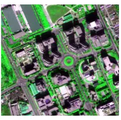
To evaluate the performance of proposed shadow detection method, we chose three pieces of remote sensing urban images among which the main variation is the complexity of scenes contents (Figures 1-4).

Image 1: The first image is acquired in September 2003, refers to a 280 × 280 pixel image in the visible spectrum. As shown in Figure 1, it mainly consists of grass areas, buildings, and their shadows.

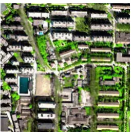
Image 2: Beijing in May 2011. The second image is scene of Beijing acquired in May 2011 and its size is 300×300. It mainly contains trees, grass, buildings, blue roofs, and shadows.

[image:5.595.313.435.441.562.2]

Image 3: Beijing in April 2011. The second image is scene of Beijing acquired in May 2011 and its size is 300×300. The land covers in it are same with Image 2, except for roads.

Figure 1. First image.

[image:6.595.314.436.69.193.2]

DOI: 10.4236/jsip.2019.104011 205 Journal of Signal and Information Processing

Figure 3. Beijing in April 2004.

Figure 4. Wuhan University in 2004.

Image 4: Wuhan University in 2004. The fourth image represents a crop of 256 × 256 pixels of the Wuhan University acquired in 2004. There are six land covers: roads, bared land, trees, buildings, water, and shadows.

3.2. Compression Approaches

To verify the superiority of the proposed shadow detection method to the ones without edge constraints, three methods are employed as the competitors: bith-reshold method [7], PCAHSI [8], and soft Shadow Detection method [12].

Bithreshold method

Bithreshold method tries to use two spectral features of shadow areas. Firstly, transform the image into HIS color space, compute the normalized difference of intensity (𝐼𝐼) and saturation (𝑆𝑆) components, and obtain the initial detection by its threshold. Then, get the detection result of 𝐼𝐼 channel by histogram threshold. The final result is obtained by performing AND operation on two detected re-sults mentioned above.

PCAHSI

Firstly, compute the shadow index (SI) based on principal component trans-formation and HIS model. Then, image is divided into the shadow area and nonshadow area by SI histogram threshold.

Soft shadow

[image:6.595.310.438.217.346.2]

proba-DOI: 10.4236/jsip.2019.104011 206 Journal of Signal and Information Processing bility is employed as the class conditional probability and an iterative procedure based on MRF is used to segment the image into shadow areas and the nonsha-dows.

3.3. Experiments and Discussion

In this section, the performance of the proposed method is verified by experi-mental results. Some parameters in our experiments were chosen empirically. In detail, β =0.3 for Potts model and α=0.2 for soft edge indicator. Another important parameter, the window size of neighborhood for HMRF is set as 3 × 3 because it can preserve as much as possible the image details.

Visual Comparison

Experimental results on the first image using different methods (bi-threshold, PCA method, soft shadow method, the proposed method) are shown in Figure 5. Figure 5(e) is the ground truth of image 1.

Obviously, there are many misdetection in Figure 5(a) and Figure 5(b) be-cause these two methods only used thershold of spectual features. It is not effi-cient enough to distinguish dark objects from shadows. These defects are re-moved in soft shadow method shown in Figure 5(c), which thanks for the soft shadow model. Also because of the use of HMRF, soft shadow method obtained more homogenous regions. But, region boundaries in Figure 5(c) are so smooth that some details are missing, even some trivial shadow areas. Seen from Figure 5(d), the proposed method is superior to the competitive ones. It can obtain more accurate boundaries as well as homogenous regions for the constrainsts of edgs. These comparisons can also be presented in Figure 6, Figure 7 and Figure 8. From the comparison of results of four images, we can see that as the complexity

(a) (b) (c)

(d) (e)

DOI: 10.4236/jsip.2019.104011 207 Journal of Signal and Information Processing

(a) (b) (c)

[image:8.595.225.522.68.288.2]

(d) (e)

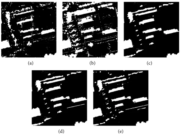
Figure 6. Detection results of Image 2. (a) Bi-threshold; (b) PCA; (c) Soft shadow; (d) The proposed method; (e) The ground truth.

(a) (b) (c)

[image:8.595.211.538.324.565.2]

(d) (e)

Figure 7. Detection results of Image 3. (a) Bi-threshold method; (b) PCA method; (c) Soft shadow method; (d) The proposed method; (e) The ground truth.

DOI: 10.4236/jsip.2019.104011 208 Journal of Signal and Information Processing

[image:9.595.271.476.69.179.2]

(d) (e)

Figure 8. Detection results of Image 4. (a) Bi-threshold method; (b) PCA method; (c) Soft shadow method; (d) The proposed method; (e) The ground truth.

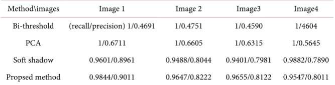
Table 1. Recall and precision.

Method\images Image 1 Image 2 Image3 Image4 Bi-threshold (recall/precision) 1/0.4691 1/0.4751 1/0.4590 1/4604 PCA 1/0.6711 1/0.6605 1/0.6315 1/0.5645 Soft shadow 0.9601/0.8961 0.9488/0.8044 0.9401/0.7981 0.9882/0.7890 Propsed method 0.9844/0.9011 0.9647/0.8222 0.9655/0.8122 0.9547/0.8011

of land covers increases, the greater misdetection occurs. Quantitative Comparisons

To obtain a quantitative comparison between different algorithms, both recall and precision are employed as the performance metrics. Recall represents how many true shadow pixels have been detected as shadow pixels, which is denoted by

100%

c

t

N DR

N

= × ₍₈₎

where Nt is the number of true shadow pixels, while Nc is the number of

pixels detected as shadows correctly. Nc is computed by performing AND

op-eration on the detected result and the true shadow mask.

Precision indicates that in the detected shadow pixels, how many correct ones are there. It can be denoted as:

100%

c

d

N DP

N

= ×

₍₉₎

where Nd is the number of pixels labeled as shadow. From the definition, it is

easy to conclude that the recall favors over detection and the precision favors under detection. That is to say, high recall combined with a low precision means over detection shadows. We measured the recall and precision of each method and listed their values in Table 1. From the quantitative results as shown in Ta-ble 1, it is easy to conclude that the proposed method can obtain more accurate shadow detection results than the competitors.

4. Conclusion

[image:9.595.206.540.243.328.2]

DOI: 10.4236/jsip.2019.104011 209 Journal of Signal and Information Processing model is put forward, considering the fact that shadow edges are not discrimi-nate clearly. Based on this, an iterative shadow detection method with edge con-straints based on HMRF is proposed. Experiments on remote sensing images have illustrated that the proposed method can get more clearly edges as well as homogenous regions.

Funding

This work is supported in part by the National Natural Science Foundation of China under Grants 41001251, the Key Technology Projects of Henan province of China (No. 132102210212), the Key Technology Projects of the Educational Department of Henan Province of China (No. 16A520036).

Conflicts of Interest

The author declares no conflicts of interest regarding the publication of this pa-per.

References

[1] Jaynes, C., Webb, S., Steele, R.M., Brown, M. and Seales, W.B. (2001) Dynamic Shadow Removal from Front Projection Displays. Proceedings of the IEEE Confe-rence on Visualization, San Diego, CA, 21-26 October 2001, 175-182.

https://doi.org/10.1109/VISUAL.2001.964509

[2] Polidorio, A.M., Flores, F.C., Imai, N.N., Tommaselli, A.M.G. and Franco, C. (2003) Automatic Shadow Segmentation in Aerial Color Images. Proceedings of the 16th Brazilian Symposium on Computer Graphics and Image Processing, Sao Carlos, 12-15 October 2003, 270-277. https://doi.org/10.1109/SIBGRA.2003.1241019 [3] Huang, J., Xie, W. and Tang, L. (2004) Detection of and Compensation for Shadows

in Colored Urban Aerial Images. Proceedings of the 5th World Congress on Intelli-gent Control and Automation, June 2004, 3098-3100.

[4] Ma, H.J., Qin, Q.M. and Shen, X.Y. (2008) Shadow Segmentation and Compensa-tion in High ResoluCompensa-tion Satellite Images. Proceedings of the IEEE International Geoscience and Remote Sensing Symposium, Boston, MA, 7-11 July 2008, 1036- 1039.

[5] Arevalo, V., Gonzalez, J. and Ambrosio, G. (2008) Shadow Detection in Color High-Resolution Satellite Images. International Journal of Remote Sensing, 29, 1945-1963.https://doi.org/10.1080/01431160701395302

[6] Tsai, V.J.D. (2006) A Comparative Study on Shadow Compensation of Color Aerial Images in Invariant Color Models. IEEE Transactions on Geoscience and Remote Sensing, 44, 1661-1671.https://doi.org/10.1109/TGRS.2006.869980

[7] Yang, J., Zhao, Z. and Yang, J. (2008) A Shadow Removal Method for High Resolu-tion Remote Sensing Image. Geomatics and Information Science of Wuhan Univer-sity, 33, 17-20.

[8] Liu, H. and Xie, T. (2013) Study on Shadow Detection in High Resolution Remote Sensing Image of PCA and HIS Model. Remote Sensing Technology and Applica-tion, 28, 78-84.

DOI: 10.4236/jsip.2019.104011 210 Journal of Signal and Information Processing https://doi.org/10.1109/ICIP.2014.7026020

[10] Wang, C., Liu, J., Gong, M., Jiao, L. and Liu, J. (2014) Fuzzy c-Means Clustering with Weighted Energy Function in MRF for Image Segmentation. 2014 IEEE Inter-national Conference on Fuzzy System (Fuzzy-IEEE), Beijing,6-11 July 2014, 210-215. https://doi.org/10.1109/FUZZ-IEEE.2014.6891657

[11] Liu, G., Zhang, Y. and Wang, A. (2015) Incorporating Adaptive Local Information into Fuzzy Clustering for Image Segmentation. IEEE Transactions on Image Pro- cessing, 24, 3990-4000.https://doi.org/10.1109/TIP.2015.2456505

[12] Ge, W.Y. and Liu, G.Y. (2018). Unsupervised Classification of High-Resolution Remote-Sensing Images under Edge Constraints. Pattern Recognition and Com-puter Vision.https://doi.org/10.1117/12.2285777

[13] Chatzis, S.P. and Varvarigou, T.A. (2008) A Fuzzy Clustering Approach toward Hidden Markov Random Field Models for Enhanced Spatially Constrained Image Segmentation. IEEE Transactions on Fuzzy Systems, 16, 1351-1361.