Volume 365, Number 11, November 2013, Pages 5859–5881 S 0002-9947(2013)05804-7
Article electronically published on April 25, 2013
GEOMETRIC GRID CLASSES OF PERMUTATIONS
MICHAEL H. ALBERT, M. D. ATKINSON, MATHILDE BOUVEL, NIK RUˇSKUC, AND VINCENT VATTER
Abstract. A geometric grid class consists of those permutations that can be
drawn on a specified set of line segments of slope±1 arranged in a rectangular pattern governed by a matrix. Using a mixture of geometric and language theoretic methods, we prove that such classes are specified by finite sets of for-bidden permutations, are partially well ordered, and have rational generating functions. Furthermore, we show that these properties are inherited by the subclasses (under permutation involvement) of such classes, and establish the basic lattice theoretic properties of the collection of all such subclasses.
1. Introduction
Subsequent to the resolution of the Stanley-Wilf Conjecture in 2004 by Marcus and Tardos [21], two major research programmes have emerged in the study of permutation classes:
• to characterise the possible growth rates of permutation classes and
• to provide necessary and sufficient conditions for permutation classes to have amenable generating functions.
With regard to the first programme, we point to the work of Kaiser and Klazar [20], who characterised the possible growth rates up to 2, and the work of Vatter [25], who extended this characterisation up to the algebraic numberκ≈2.20557, the point at which infinite antichains begin to emerge, and where the transition from countably many to uncountably many permutation classes occurs. The second programme is illustrated by the work of Albert, Atkinson, and Vatter [3], who showed that all subclasses of the separable permutations not containing Av(231) or a symmetry of this class have rational generating functions.
Both research programmes rely on structural descriptions of permutation classes, in particular, the notion of grid classes. Here we study the enumerative and order-theoretic properties of a certain type of grid class called a geometric grid class.
While we present formal definitions in the next two sections, geometric grid classes may be defined briefly as follows. Suppose thatM is a 0/±1 matrix. The
standard figure of M, which we typically denote by Λ, is the point set inR2 con-sisting of:
• the increasing open line segment from (k−1, −1) to (k, ) ifMk,= 1 or
• the decreasing open line segment from (k−1, ) to (k, −1) ifMk,=−1. (Note that in order to simplify this correspondence, we index matrices first by col-umn, counting left to right, and then by row, counting bottom to top throughout.)
Received by the editors August 31, 2011 and, in revised form, January 30, 2012. 2010Mathematics Subject Classification. Primary 05A05, 05A15.
c
2013 American Mathematical Society
3 5
1 6
2 4
1 5
3 4
[image:2.504.143.363.80.184.2]2 6
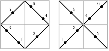
Figure 1. The permutation 351624 on the left and the permu-tation 153426 on the right lie, respectively, in the geometric grid
classes of
1 −1
−1 1
and
−1 1 1 −1
.
Thegeometric grid class ofM, denoted by Geom(M), is then the set of all permu-tations that can be drawn on this figure in the following manner. Choosenpoints in the figure, with no two on a common horizontal or vertical line. Then label the points from 1 to nfrom bottom to top and record these labels reading from left to right.
Much of our perspective and inspiration comes from Steve Waton, who consid-ered two particular geometric grid classes in his thesis [28]. These are the permu-tations which can be drawn from a circle, later studied by Vatter and Waton [27], and the permutations which can be drawn on an X, later studied by Elizalde [12]. Examples of these two grid classes are shown in Figure 1.1
A permutation class is said to be geometrically griddable if it is contained in some geometric grid class. With that final piece of terminology, we can state the main results of this paper.
• Theorem 6.1. Every geometrically griddable class is partially well ordered.
(Such classes do not contain infinite antichains.)
• Theorem 6.2. Every geometrically griddable class is finitely based. (These
classes can be defined by only finitely many forbidden patterns.)
• Theorem 8.1. Every geometrically griddable class is in bijection with a
regular language and thus has a rational generating function.
• Theorem 9.1. The simple, sum indecomposable, and skew indecomposable
permutations in every geometrically griddable class are each in bijection with a regular language and thus have rational generating functions.
• Theorem 10.3. The atomic geometrically griddable classes are precisely
the geometric grid classes of •-isolated 0/•/±1 matrices, and every geo-metrically griddable class can be expressed as a finite union of such classes.
(This type of geometric grid class is defined in Section 10.)
For the remainder of the introduction we present the (standard) definitions of permutation classes. In the next section we formalise the geometric notions of
1The drawing on the left of Figure 1 has been drawn as a diamond to fit with the general
this paper. Section 3 contains a brief discussion of grid classes of forests, while Section 4 introduces partial multiplication matrices. Sections 5–10 introduce a correspondence between permutations in a geometric grid class and words, and utilise this correspondence to establish the main results of the paper. Finally, in Section 11, we conclude with numerous open problems.
The permutation π of {1,2, . . . , n} contains or involves the permutation σ of
{1,2, . . . , k} (written σ ≤ π) if π has a subsequence of length k which is or-der isomorphic to σ. For example, π = 391867452 (written in list, or one-line notation) contains σ = 51342, as can be seen by considering the subsequence
π(2)π(3)π(5)π(6)π(9) = 91672. A permutation class is a downset of permuta-tions under this containment ordering; thus ifC is a permutation class,π∈ C, and
σ≤π, then σ∈ C.
For any permutation classC there is a unique (and possibly infinite) antichain
B such that
C= Av(B) ={π:β≤πfor allβ ∈B}.
This antichain B is called thebasis ofC. We denote byCn (forn∈N) the set of permutations inC of lengthn, and we refer to
∞
n=0
|Cn|xn=
π∈C
x|π|
as thegenerating function ofC.
Finally, a permutation class, or indeed any partially ordered set, is said to be
partially well ordered (pwo) if it contains neither an infinite strictly descending chain nor an infinite antichain. Of course, permutation classes cannot contain infinite strictly descending chains, so in this context being pwo is equivalent to having no infinite antichain.
2. The geometric perspective
Geometric ideas play a significant role in this paper, and to provide background we reintroduce permutations and the involvement relation in a somewhat nonstan-dard manner.
We call a subset of the plane afigure. We say that the figureF ⊆R2 isinvolved in the figure G, denoted F ≤ G, if there are subsets A, B ⊆ R and increasing injectionsφx:A→Randφy :B→Rsuch that
F ⊆A×B andφ(F) ={(φx(a), φy(b)) : (a, b)∈ F} ⊆ G.
The involvement relation is apreorder (it is reflexive and transitive but not neces-sarily antisymmetric) on the collection of all figures. IfF ≤ G andG ≤ F, then we say that F and G are (figure) equivalent and writeF ≈ G. Note that in the case of figures with only finitely many points, two figures are equivalent if and only if one can be transformed to the other by stretching and shrinking the axes. Three concrete examples are provided below.
• The figuresF={(a,|a|) : a∈R}andG={(a, a2) : a∈R}are equivalent. To see thatF ≤ G, takeA×B=R×R≥0,φx(a) =a, andφy(b) =b2. To see thatG ≤ F, takeA×B=R×R≥0,φx(a) =a, andφy(b) =
√ b.
• The figuresF ={(a, a) : a∈R} and G={(a, a) : a∈[0,1]∪[2,3]}are equivalent. To see thatF ≤ G, takeA×B=R2,φ
φy(b) = 1/(1 +e−b). To see that G ≤ F, consider the identity map with
A×B= ([0,1]∪[2,3])2.
• The “unit diamond” defined by F={(a, b) : |a|+|b|= 1}(shown on the left of Figure 1) is equivalent to the unit circle G={(a, b) : a2+b2= 1}. To see that F ≤ G, takeA×B= [−1,1]2, φ
x(a) = sin(πa/2), andφy(b) = cos(π(1−b)/2). To see that G ≤ F, simply consider the inverses of these maps.
To any permutation π of lengthn, we associate a figure which we call its plot,
{(i, π(i))}. These figures have the important property that they are independent, by which we mean that no two points lie on a common horizontal or vertical line. It is clear that every finite independent figure is equivalent to the plot of a unique permutation, so we could define a permutation as an equivalence class of finite independent figures. Under this identification, the partial order on equivalence classes of finite independent figures is the same as the containment, or involvement, order defined in the introduction.
Every figureF ⊆R2therefore naturally defines a permutation class,
Sub(F) ={permutations π : πis equivalent to a finite independent subset ofF}.
For example:
• LetF ={(x, x) : x∈R}. Then Sub(F) contains a single permutation of each length, namely the identity, and its basis is{21}.
• LetF={(x, x) : x∈[0,1]}∪{(x+1, x) :x∈[0,1]}. Then Sub(F) consists of all permutations having at most one descent. Its basis is{321,2143,3142}, as can be seen by considering the ways in which two descents might occur.
• Let F = {(x,sin(x)) : x ∈ R}. Then Sub(F) is the set of all permuta-tions. To establish this, note that every permutation can be broken into its increasing contiguous segments (“runs”) and points corresponding to each run can be chosen from increasing segments of F. Its basis is, of course, the empty set.
A geometric grid class (as defined in the introduction) is precisely Sub(Λ), where Λ denotes the standard figure of the defining matrix. Permutation classes of the form Sub(F) in the special case whereF is the plot of a bijection between two subsets of the real numbers have received some study before; we refer the reader to Atkinson, Murphy, and Ruˇskuc [7] and Huczynska and Ruˇskuc [18].
The lines {x=k : k= 0, . . . , t} and{y= : = 0, . . . , u} play a special role for standard figures, as they divide the figure into its cells. We extend this notion ofgriddings to all figures. First, though, we need to make a technical observation: because the real number line is order isomorphic to any open interval, it follows that every figure is equivalent to a bounded figure, and thus we may restrict our attention to bounded figures.
LetR= [a, b]×[c, d] be a rectangle inR2. At×u-gridding ofRis a tuple
G= (g0, g1, . . . , gt;h0, h1, . . . , hu)
of real numbers satisfying
a=g0≤g1≤ · · · ≤gt=b,
C11 C21 C31
C12 C22 C32
a g1 g2 b
c h1
[image:5.504.168.332.74.187.2]d
Figure 2. A 3×2 gridding of the rectangle [a, b]×[c, d] with the cells Ck, indicated.
These numbers are identified with the corresponding set of vertical and horizontal lines partitioningRinto a rectangular collection of cellsCk, as shown in Figure 2. We often identify the gridding Gand the collection of cellsCk,.
A gridded figure is a pair (F, G), where F is a figure and Gis a gridding con-taining F in its interior. To ensure that each point of F lies in a unique cell, we also require that the grid lines are disjoint fromF. By analogy with ungridded fig-ures and permutations, we define the preorder≤and the equivalence relation≈for
t×ugridded figures. The additional requirement is that the mappingφ= (φx, φy) appearing in the original definition maps the (k, ) cell of one gridded figure to the (k, ) cell of the other gridded figure. Agridded permutationis the equivalence class of a finite independent gridded figure.
The connection between finite figures, gridded finite figures, permutations, and gridded permutations can be formalised as follows. Let Φ and Φ, respectively, denote the set of all finite independent and finite gridded independent figures in R2, and letSandS, respectively, denote the set of all permutations and all gridded permutations. The (obvious) mappings connecting these sets are:
• Δ : Φ→Φ, given by removing the grid lines, i.e., (F, G)→ F;
• δ : S → S, also given by removing the grid lines, i.e., in this context, mapping the equivalence class of (F, G) under ≈to the equivalence class ofF under ≈;
• π : Φ → S, which sends every element of Φ to its equivalence class under ≈;
• π : Φ→ S, which sends each element of Φ to its equivalence class under
≈.
It is a routine matter to verify that the diagram
Φ Φ
S S
Δ
δ
π π
commutes.
compatible withM if the following holds for all relevantkand:
F ∩Ck, is
⎧ ⎨ ⎩
increasing, ifMk,= 1, decreasing, ifMk,=−1, empty, ifMk,= 0.
We are concerned with the images, under the maps π and πΔ =δπ, of the set of allM-compatible, finite, independent, gridded figures. We denote these two sets by Grid(M) and Grid(M), respectively. We refer to Grid(M) as the(monotone) grid class ofM.
In this context, the standard figure Λ (as defined in the introduction) of a 0/±1 matrixM of sizet×uhasstandard grid linesGgiven by{x=k :k= 0, . . . , t}and
{y = : = 0, . . . , u}. We refer to the pair (Λ, G) as thestandard gridded figure
of M and denote it by Λ; note that Λ is compatible (in the sense above) with
M. The set of all gridded permutations contained in Λis denoted by Geom (M), and its image under δ is Geom(M), as defined in the introduction. Because the standard gridded figure of a 0/±1 matrixM is compatible withM, we always have
Geom(M)⊆Grid(M).
In the next section we characterise the matrices for which equality is achieved.
3. Grid classes of forests
The first appearance of grid classes in the literature, in the special case whereM
is a permutation matrix and under the name “profile classes”, was in Atkinson [5]. Atkinson observed that such grid classes have polynomial enumeration. Huczynska and Vatter [19], who introduced the name “grid classes”, generalised Atkinson’s result to show that grid classes of signed permutation matrices have eventually polynomial enumeration. This result allowed them to give a more structural proof of Kaiser and Klazar’s “Fibonacci dichotomy” [20], which states that for every permutation class C, either|Cn|is greater than thenth Fibonacci number for alln or |Cn|is eventually polynomial.
Atkinson, Murphy, and Ruˇskuc [6] and Albert, Atkinson, and Ruˇskuc [2] studied the special case of grid classes of 0/±1 vectors, under the name “W-classes”. The former paper proves that such grid classes are pwo and finitely based, while the latter shows that they have rational generating functions.
The first appearance of grid classes of 0/±1 matrices in full generality was in Murphy and Vatter [22] (again under the name “profile classes”). They were in-terested in the pwo properties of such classes, and to state their result we need a definition.
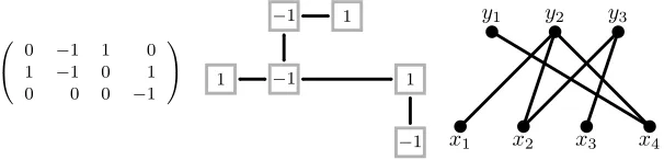
The cell graph of M is the graph on the vertices {(k, ) : Mk, = 0} in which (k, ) and (i, j) are adjacent if the corresponding cells ofM share a row or a column and there are no nonzero entries between them in this row or column. We say that the matrix M is a forest if its cell graph is a forest. Viewing the absolute value ofM as the adjacency matrix of a bipartite graph, we obtain a different graph, its
row-column graph.2 It is not difficult to show that the cell graph of a matrix is a forest if and only if its row-column graph is also a forest. An example of each
2In other words, the row-column graph of a t×umatrix M is the bipartite graph on the
⎛
⎝ 01 −−11 10 01
0 0 0 −1
⎞
⎠ 1 −1
−1 1
1
−1 x1 x2 x3 x4
[image:7.504.101.404.81.154.2]y1 y2 y3
Figure 3. A matrix together with its cell graph (centre) and row-column graph (right).
of these graphs is shown in Figure 3. These graphs completely determine the pwo properties of grid classes:
Theorem 3.1 (Murphy and Vatter [22], later generalised by Brignall [10]). The
class Grid(M)is pwo if and only ifM is a forest.
It has long been conjectured that Grid(M) has a rational generating function if
M is a forest;3for example, by Huczynska and Vatter [19, Conjecture 2.8]. Indeed, this conjecture was the original impetus for the present work. However, as the work progressed, it became apparent that the geometric paradigm provided a viewpoint which was at once more insightful and more general, and thus our perspective shifted. The link with the original motivation is provided by the following result.
Theorem 3.2. IfM is a forest, thenGrid(M) = Geom(M)and thusGrid(M) =
Geom(M).
Proof. The proof is by induction on the number of nonzero entries of M. For the case of a single nonzero cell, note that one can place any increasing (resp., decreasing) set of points on a line of slope 1 (resp., −1) by applying a horizontal transformation.
Now suppose thatM has two or more nonzero entries, denote its standard grid-ded figure by ΛM = (ΛM, G), and let (k, ) denote a leaf in the cell graph ofM. By considering the transpose ofM if necessary, we may assume that there are no other nonzero entries in column kofM. Letπ be an arbitrary gridded permutation in Grid(M). We aim to show thatπ∈Geom
(M).
Denote byN the matrix obtained fromM by setting the (k, ) entry equal to 0, and denote its standard gridded figure by ΛN = (ΛN, G). Note that the grid lines of ΛN and Λ
M are identical because the corresponding matrices are the same size. Let
σ denote the gridded permutation obtained fromπby removing all entries in the (k, ) cell. Becauseσ lies in Grid
(N), which by induction is equal to Geom(N), there is a finite independent point set S ⊆ΛN ⊆ΛM such that (S, G)≈σ. As long as we do not demand that the new points belong to ΛM, it is clear that we can extendS by adding points in the (k, ) cell to arrive at a point setP⊇S such that (P, G)≈π. Then we can apply a horizontal transformation to column kto move these new points onto the diagonal line segment of ΛM in this cell. This horizontal transformation does not affect the points ofS, because none of those points lie in column k, so we see thatP ⊆ΛM, and thusπ∈Geom(M), as desired.
3Note that Grid(M) can have a nonrational generating function whenM is not a forest. An
2 4
[image:8.504.101.397.77.298.2]1 3
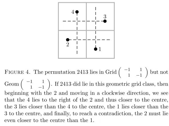
Figure 4. The permutation 2413 lies in Grid
−1 1 1 −1
but not
Geom
−1 1 1 −1
. If 2413 did lie in this geometric grid class, then
beginning with the 2 and moving in a clockwise direction, we see that the 4 lies to the right of the 2 and thus closer to the centre, the 3 lies closer than the 4 to the centre, the 1 lies closer than the 3 to the centre, and finally, to reach a contradiction, the 2 must lie even closer to the centre than the 1.
Because of Theorem 3.2, all of our results about geometric grid classes yield immediate corollaries to grid classes of forests, which we shall generally not mention. For example, our upcoming Theorem 6.1 generalises one direction of Theorem 3.1. The fact that Grid(M) is not pwo whenM is not a forest (the other direction of Theorem 3.1), combined with Theorem 6.1 which shows that all geometric grid classes are pwo, implies that the converse to Theorem 3.2 also holds: if Grid(M) = Geom(M), then M is a forest. This fact can also be established by arguments generalising those accompanying Figure 4.
4. Partial multiplication matrices
In this section we consider a particular “refinement” operation on matrices, which is central to our later arguments. Let M be a 0/±1 matrix of size t×u and
q be a positive integer. The refinement M×q of M is the 0/±1 matrix of size
qt×qu obtained from M by replacing each 1 by a q×q identity matrix (which, by our conventions, has ones along its southwest-northeast diagonal), each −1 by a negative q×qanti-identity matrix, and each 0 by a q×qzero matrix. It is easy to see that the standard figure M×q is equivalent to the standard figure ofM, so Geom(M×q) = Geom(M) for all q(although, of course, the corresponding gridded classes differ).
The refinementsM×2 play a special role throughout this paper. To explain this we first need a definition. We say that a 0/±1 matrix M of sizet×uis a partial multiplication matrix if there arecolumn and row signs
c1, . . . , ct, r1, . . . , ru∈ {1,−1}
such that every entryMk, is equal to either 0 or the productckr.
As our next result shows, we are never far from a partial multiplication matrix.
Proposition 4.1. For every 0/±1 matrix M, its refinement M×2 is a partial
Proof. By construction,M×2 is made up of 2×2 blocks equal to
0 0 0 0
,
0 1 1 0
, and
−1 0 0 −1
.
From this it follows that (M×2)
k, ∈ {0,(−1)k+}. Therefore we may take ck = (−1)k andr
= (−1)as our column and row signs.
Because Geom(M) = Geom(M×2), we may always assume that the matrices we work with are partial multiplication matrices. We record this useful fact below.
Proposition 4.2. Every geometric grid class is the geometric grid class of a partial
multiplication matrix.
5. Words and encodings
From the point of view of our goals in this paper, subword-closed languages over a finite alphabet display model behaviour: all such languages are defined by finite sets of forbidden subwords, are pwo under the subword order, and have rational generating functions. The brunt of our subsequent effort is focused on transferring these favourable properties from words to permutations.
Let Σ be a finite alphabet and Σ∗ be the set of all finite words (i.e., sequences) over Σ. This set is partially ordered by means of thesubword orsubsequence order:
v≤wif one can obtainv fromwby deleting letters.
Subsets of Σ∗ are called languages. We say that a language issubword-closed if it is a downward closed set in the subword order (such languages are also called
piecewise testable by some; for example, Simon [23]). To borrow terminology from permutation classes, we say that the basis of a subword-closed language L is the set of minimal words which do not lie in L. It follows that Lconsists of precisely those words which do not contain any element of its basis. Moreover, a special case of a result of Higman [15] implies that subword-closed languages have finite bases:
Higman’s Theorem. The set of words over any finite alphabet is pwo under the
subword order.
The following characterisation of subword-closed languages is folkloric and fol-lows directly from the fact that, for any finite set of forbidden subwords, there exists a finite state automaton accepting words not containing these subwords, which is acyclic except for loops at individual states.
Proposition 5.1. Let Σbe a finite alphabet. Every nonempty subword-closed
lan-guage over Σcan be expressed as a finite union of languages of the form
Σ∗1{ε, a2}Σ∗3{ε, a4}. . .Σ∗2q−1{ε, a2q}Σ∗2q+1,
whereq≥0,a2, . . . , a2q∈ΣandΣ1, . . . ,Σ2q+1⊆Σ.
This fact shows that subword-closed languages areregular languages. To recall their definition briefly, given a finite alphabet Σ, the empty language∅, the empty word language {ε}, and the singleton languages {a} for each a ∈ Σ are regular. Moreover, given two regular languages K and Lover Σ, their union K∪L, their concatenationKL={vw : v∈K andw∈L}, and the starL∗={v(1)· · ·v(m) :
p1
p2
p3
p4
p5
p6
[image:10.504.173.330.74.182.2]p7
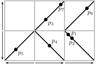
Figure 5. An example of the mapϕfor a matrix with row signs
r1=−1 andr2= 1 and column signsc1=−1,c2=c3= 1. Here we see thatϕ(a31a31a22a21a11a32a22) = 1527436.
their complement K\L is also regular, a property we use many times. We say that the generating function of the language Lis x|w|, where the sum is taken over all w∈L and|w| denotes the number of letters inw, i.e., itslength. We use only the most basic properties of regular languages, for which we refer the reader to Flajolet and Sedgewick [13, Section I.4 and Appendix A.7]. In particular, the following fact is of central importance throughout the paper.
Theorem 5.2. Every regular language has a rational generating function.
We now describe the correspondence between permutations in a geometric grid class, Geom(M), and words over an appropriate finite alphabet. This encoding, essentially introduced by Vatter and Waton [26], is fundamental to all of our proofs. By Proposition 4.2, we may assume thatM is at×upartial multiplication matrix with column and row signs c1, . . . , ct and r1, . . . , ru. Let Λ denote the standard gridded figure ofM, and define thecell alphabet ofM to be
Σ ={ak : Mk,= 0}.
Intuitively, the letterakrepresents an instruction to place a point in an appropriate position on the line in the (k, ) cell of Λ. This appropriate position is determined as follows, and the whole process is depicted in Figure 5.
We say that the base line of a column of Λ is the grid line to the left (resp., right) of that column if the corresponding column sign is 1 (resp., −1). Similarly, the base line of a row of Λ is the grid line below (resp., above) that row if the corresponding row sign is 1 (resp., −1). We designate the intersection of the two base lines of a cell as itsbase point. Note that the base point is an endpoint of the line segment of Λ lying in this cell. As this definition indicates, we interpret the column and row signs as specifying the direction in which the columns and rows are “read”. Owing to this interpretation, we represent the column and row signs in our figures by arrows, as shown in Figure 5.
To every wordw=w1· · ·wn∈Σ∗ we associate a permutationϕ(w) as follows. First we choose arbitrary distances
0< d1<· · ·< dn<1.
Next, for each i, we let pi be the point on the line segment in cell Ck,, where
our choice of distances d1, . . . , dn that p1, . . . , pn are independent, and we define
ϕ(w) to be the permutation which is equivalent to the set{p1, . . . , pn} of points. It is a routine exercise to show that ϕ(w) does not depend on the particular choice of distances d1, . . . , dn, showing that the mappingϕ : Σ∗ →Geom(M) is well defined. Of course there is a gridded counterpart ϕ : Σ∗ → Geom
(M), whereby we retain the grid lines coming from the figure Λ.
The basic properties of ϕandϕ are described by the following result.
Proposition 5.3. The mappings ϕ and ϕ are length-preserving, finite-to-one,
onto, and order-preserving.
Proof. Thatϕis length-preserving is obvious, as it maps letters in a word to entries in a permutation; that it is finite-to-one follows immediately from this.
In order to prove that ϕ is onto, let π ∈ Geom(M) and choose a finite set
P ={p1, . . . , pn} ⊆ Λ of points which represent π (where as usual Λ denotes the standard figure of M). Suppose that the pointpi belongs to the cell (ki, i) of Λ, and let di denote the infinity-norm distance frompi to the base point of this cell. The points in P are independent because they are equivalent to a permutation. Therefore, we may move the points of P independently by small amounts without affecting its (figure) equivalence class, and thus may assume that the distances
di are distinct. By reordering the points if necessary, we may also assume that
d1<· · ·< dn. It is then clear thatϕ(ak11· · ·aknn) =π, so ϕis indeed onto.
It remains to show that ϕis order-preserving. Suppose that v =v1· · ·vk, w =
w1· · ·wn ∈Σ∗ satisfyv ≤w. Thus there are indices 1 ≤i1 <· · ·< ik ≤n such that v=wi1· · ·wik. Note that ifϕ(w) is represented by the point set{p1, . . . , pn}
via the sequence of distances d1<· · ·< dn, thenϕ(v) is represented by the point set {pi1, . . . , pik}via the sequence of distancesdi1 <· · ·< dik, soϕ(v)≤ϕ(w).
The proofs for the gridded versionϕ are analogous.
Using this correspondence between words and permutations, one may give an alternative proof of Theorem 3.2, showing that Grid(M) = Geom(M) and thus that Grid(M) = Geom(M) whenM is a forest. As Proposition 5.3 shows thatϕ
maps onto Geom(M), one only needs to show that it also maps onto Grid(M) whenM is a forest. This is proved directly in Vatter and Waton [26].
6. Partial well order and finite bases
We now use the encoding ϕ : Σ∗ → Geom(M) from the previous section to establish structural properties of geometrically griddable classes, i.e., subclasses of geometric grid classes. We begin with partial well order. By Theorem 3.2, this generalises one direction of Theorem 3.1.
Theorem 6.1. Every geometrically griddable class is partially well ordered.
Proof. LetCbe a geometrically griddable class. By Proposition 4.2,C ⊆Geom(M) for some partial multiplication matrix M. As partial well order is inherited by subclasses, it suffices to prove that Geom(M) is pwo. Let ϕ : Σ∗ →Geom(M), where Σ is the cell alphabet ofM, be the encoding introduced in Section 5. Take
Our next goal is the following result.
Theorem 6.2. Every geometrically griddable class is finitely based.
We first make an elementary observation.
Proposition 6.3. The union of a finite number of geometrically griddable classes
is geometrically griddable.
Proof. Let C and D be geometrically griddable classes. Thus there are matrices
M and N such that C ⊆Geom(M) and D ⊆Geom(N). It follows that C ∪ D ⊆ Geom(P) for any matrixP which contains copies of bothM andN. The result for
arbitrary finite unions follows by iteration.
Given any permutation class C, we letC+1 denote the class ofone-point
exten-sions of elements ofC, that is,C+1 is the set of all permutations πwhich contain an entry whose removal yields a permutation in C. Every basis element of a class
C is necessarily a one-point extension ofC because the removal of any entry of a basis element of C yields a permutation in C. Since bases of permutation classes are necessarily antichains, Theorem 6.2 will follow from the following result and Theorem 6.1.
Theorem 6.4. If the classC is geometrically griddable, then the class C+1 is also
geometrically griddable.
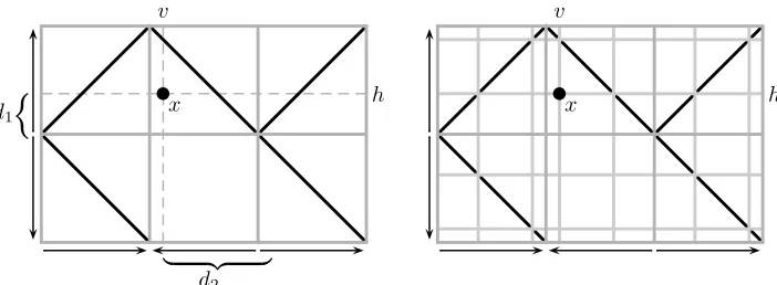
Proof. It suffices to prove the result for geometric grid classes themselves, and by Proposition 4.2 we may further restrict our attention to the case of Geom(M) where M is a partial multiplication matrix. Take τ ∈ Geom(M)+1 to be a one-point extension ofπ∈Geom(M). Letting Λ= (Λ, G) denote the standard gridded figure ofM, there is a finite independent setP ⊆Λ such that (P, G) is equivalent to some gridding ofπ. Now we may add a point, sayx, toP to obtain an independent point set which is equivalent to τ. By movingxwithout affecting the equivalence class ofP∪ {x}, we may further assume thatxlies in the interior of a cell.
Lethandvdenote, respectively, the horizontal and vertical lines passing through
x, as shown on the left of Figure 6. Our goal is to create a new, refined gridding of Λ which containsv andhas grid lines.
Theoffset of a horizontal (resp., vertical) line is the distance between that line and the base line of the row (resp., column) of Λthat it slices through (recall from Section 5 that the standard gridded figure of a partial multiplication matrix has designated base lines determined by its column and row signs). From the definition of a partial multiplication matrix, it follows that if a vertical line of offset dslices a nonempty cell of Λ, it intersects the line segment in this cell precisely where the horizontal line of offsetdslices the line segment.
Because the cells of a standard gridded figure have unit width, v and h have offsets strictly between 0 and 1, say 0< d1≤d2<1. By possibly movingxslightly without affecting the equivalence class ofP∪{x}(which we may do becauseP∪{x}
is independent), we may assume that 0< d1 < d2<1. We now define our refined gridding H, an example of which is shown on the right of Figure 6. We take
x
d1
d2
v
h x
v
[image:13.504.80.431.77.206.2]h
Figure 6. On the left is the standard gridded figure of a partial multiplication matrix, together with two additional (dashed) lines intersecting at the pointx. On the right is the refinement defined in the proof of Theorem 6.4.
and in particular consists of a grid containing line segments of slope ±1, each of which runs from corner to corner in its cell. By possibly moving the points slightly, we may assume that no point of P lies on a grid line inH (althoughxlies on two such lines).
By cutting the figure Λ at the linesvandhand moving the four resulting pieces, we can create a new column and row whose cell of intersection containsx. (One can also view this as expanding the linesvandhinto a column and a row, respectively.) We can then fill this cell of intersection with a line segment of slope±1 (the choice is immaterial) running from corner to corner; clearly,xcan be shifted onto this line segment without affecting the equivalence class of P∪ {x}. The resulting gridded figure consists of line segments that run from corner to corner in their cells and is equivalent to the standard gridded figure of some partial multiplication matrix N
which is of size (3t+ 1)×(3u+ 1), from which it follows that τ ∈Geom(N). As there are only finitely many such matrices, we see that Geom+1(M) is contained in a finite union of geometric grid classes and so is geometrically griddable by
Proposition 6.3.
7. Gridded permutations and trace monoids
p2
p3
p2
p3
Figure 7. Two drawings of a particular gridding of the per-mutation 2465371. The drawing on the left is encoded as
a31a32a11a22a31a32a11, while the drawing on the right is encoded asa31a11a32a22a31a32a11.
second and third letters of the words can be interchanged without changing the gridded permutation, which corresponds to placing the pointsp2andp3at different distances from their base points.
More precisely, suppose that M is a partial multiplication matrix with cell al-phabet Σ. We say that the two words v, w ∈ Σ∗ are equivalent if one can be obtained from the other by successively interchanging adjacent letters which rep-resent independent cells. The equivalence classes of this relation therefore form a
trace monoid, which can be defined by the presentation
Σ|aijak=akaij wheneveri=kandj=.
An element of this monoid (an equivalence class of words in Σ∗) is called a trace. It is an elementary and foundational fact about presentations that two words lie in the same trace if and only if one can be obtained from the other by a finite sequence of applications of the defining relations aijak=akaij wheneveri=k and j = (Howie [17, Proposition 1.5.9 and Section 1.6]). The theory of trace monoids is understood to considerable depth; see for example Diekert [11].
Proposition 7.1. Let M be a partial multiplication matrix with cell alphabet Σ.
For wordsv, w∈Σ∗, we have ϕ(v) =ϕ(w)if and only if v andwhave the same
trace in the trace monoid ofM.
Proof. It is clear from the preceding discussion thatϕ(v) =ϕ(w) whenevervand
whave the same trace.
Now suppose thatϕ(v) =ϕ(w). We aim to prove thatvandwhave the same trace in the trace monoid of M. Clearly v andw must have the same length, say
n. We prove our assertion by induction on n. In the case wheren= 1, note that
ϕ(ak,) consists of a single point in cellCk,, so if|v|=|w|= 1, thenϕ(v) =ϕ(w) implies thatv=w, and thusvandware in the same trace trivially. Thus we assume that n≥2 and that the assertion is true for all words of lengthn−1.
Writev =v1· · ·vn and w=w1· · ·wn. Ifv1 =w1, then from the definition of
ϕ we have ϕ(v
2· · ·vn) =ϕ(w2· · ·wn), and the assertion follows by induction. Therefore we may assume thatv1=w1.
Suppose that the column and row signs ofMarec1, . . . , ctandr1, . . . , ruand that
v1=ak. While there are four cases depending on the column and row signsckand
[image:14.504.91.415.74.188.2]among the points created by following the definition ofϕ, the point corresponding tov1inϕ(v) is the leftmost point in its column and bottommost point in its row. Since ϕ(v) =ϕ(w) as gridded permutations, ϕ(w) must also contain a point in cellMk,which is the leftmost point in its column and bottommost point in its row; suppose this point corresponds to wi. Because ck = 1, the entries in columnkare placed from left to right, so wi must be the first letter ofwwhich corresponds to a cell in columnk. Similarly, wi must be the first letter ofwwhich corresponds to a cell in row. Therefore all of the lettersw1, . . . , wi−1correspond to cells which are in different rows and columns fromMk,. This shows thatwlies in the same trace as the word
w=wiw1· · ·wi−1wi+1· · ·wn=v1w1· · ·wi−1wi+1· · ·wn.
Observe that ϕ(w) =ϕ(w) and thusϕ(w) =ϕ(v). Finally, becausev andw have the same first letter, we see that v and w are in the same trace by the first case of this argument, which implies that v andw are in the same trace, proving
the proposition.
This result established, we are reduced to the task of choosing from each trace a unique representative, which is a well-understood problem.
Proposition 7.2 (Anisimov and Knuth; see Diekert [11, Corollary 1.2.3]). In any
trace monoid, it is possible to choose a unique representative from each trace in such a way that the resulting set of representatives forms a regular language.
We immediately obtain the following.
Corollary 7.3. For every partial multiplication matrix M, the (gridded) class
Geom(M)is in bijection with a regular language.
8. Regular languages and rational generating functions
We now shift our attention to the ungridded permutations in a geometrically griddable class. This is the most technical argument of the paper, and we outline the general approach before delving into the formalisation.
The crux of the issue relates to the ungridded version of the encoding mapϕand arises because it is possible thatϕ(v) =ϕ(w) for two wordsv, w∈Σ∗ even though
ϕ(v)=ϕ(w). This happens precisely whenπ=ϕ(v) =ϕ(w) admits two different griddings. To discuss these different griddings, we say that the gridded permutation (π, G)∈ Geom(M) is a Geom(M) gridding of the permutation π ∈ Geom(M). Since our goal is to establish a bijection between any geometrically griddable class
C and a regular language, if a permutation in Chas multiple Geom(M) griddings we must choose only one. To do so, we introduce a total order on the set of all such griddings of a fixed permutation πand aim to keep only those which are minimal in this order.
The problem is thus translated to that of recognising minimal Geom(M) grid-dings: Given a word w ∈ Σ∗, how can we determine if the gridded permutation
ϕ(w) represents the minimal Geom(M) gridding ofπ=ϕ(w)? If not, then there is a lesser gridding ofπ, given by someϕ(v). The fact thatϕ(v) is less thanϕ(w) is witnessed by the position of one or more particular entries which lie in different cells inϕ(v) andϕ(w).
allowed to be marked, which we designate with an overline. (Thus our marked per-mutations look like some other authors’ signed perper-mutations, although the marking is meant to convey a completely different concept.) The containment order extends naturally, whereby we make sure that the markings line up. Formally we say that the marked permutationπof lengthncontains the marked permutationσof length
k ifπhas a subsequence π(i1), π(i2), . . . , π(ik) such that:
• π(i1)π(i2)· · ·π(ik) is order isomorphic to σ (this is the standard contain-ment order) and
• for each 1≤j≤k, π(ij) is marked if and only ifσ(j) is marked.
For example, π = 391867452 contains σ = 51342, as can be seen by consider-ing the subsequence 91672. A marked permutation class is then a set of marked permutations which is closed downward under this containment order.
The mappings ϕ and ϕ can be extended in the obvious manner to order-preserving mappings ϕandϕ from (Σ∪Σ)∗ to the marked version of Geom(M), without and with grid lines, respectively, where here Σ is the marked cell alphabet {a : a∈Σ}and both mappings send marked letters to marked entries.
Theorem 8.1. Every geometrically griddable class is in bijection with a regular
language, and thus has a rational generating function.
Proof. LetCbe a geometrically griddable class. By Proposition 4.2,C ⊆Geom(M) for a partial multiplication matrixM. By Corollary 7.3, there is a regular language, sayL, such thatϕ : L→Geom
(M) is a bijection.
We begin by defining a total order on the various griddings of each permutation
π ∈ Geom(M) and thus also on the Geom(M) griddings of permutations in C. Roughly, this order prefers griddings in which the entries ofπ lie in cells as far to the left and bottom as possible or, in terms of grid lines, the order prefers griddings in which the grid lines lie as far to the right and top as possible. Suppose we have two different Geom(M) griddings of π given by the grid lines G and H. Because these griddings are different, there must be a leftmost vertical grid line or, failing that, a bottommost horizontal grid line, which moved. Note that in the former case,GandH will contain a different number of entries in the corresponding column, while in the latter case they will contain a different number of entries in the corresponding row.
Formally, if (π, G) contains the same number of entries as (π, H) in each of the leftmostk−1 columns but contains more entries than (π, H) in columnk, then we write (π, G)<(π, H), and we say that columnk witnesses this fact. Otherwise, if (π, G) and (π, H) contain the same number of entries in each column and in each of the bottom−1 rows but (π, G) contains more entries than (π, H) in row, then (π, G)<(π, H), and we say that row witnesses this fact. Given a permutation
LetC denote the set of all marked gridded permutations obtained from triples (π, G, H), π ∈ C, in this manner. Because Geom(M) griddings are inherited by subpermutations andϕ is order-preserving, the language
J =ϕ−1
C
is subword-closed in Σ∪Σ∗. In particular, J is a regular language. Loosely speaking, the words in J containing marked letters carry information about all the nonminimal griddings. Our goal is therefore to recognise these nonminimal griddings in Σ∗ and remove them from the languageL.
Consider any word w∈L, which encodes the Geom
(M)-gridded permutation
ϕ(w) = (π, H). The gridding given by H is not the minimal Geom
(M) grid-ding of π precisely if J contains a copy of w with one or more marked letters. Let Γ : Σ∪Σ∗ → Σ∗ denote the homomorphism which removes markings, i.e., the homomorphism given by a, a → a. The words which represent nonminimal griddings (precisely the words we wish to remove from L) are therefore the set
K= Γ
J∩Σ∪Σ∗\Σ∗
.
By the basic properties of regular languages, it can be seen that K and hence
L=L\Kare regular. The proof is then complete, asϕ:L→ Cis a bijection.
9. Indecomposable and simple permutations
Here we adapt the techniques of the previous section to establish bijections be-tween regular languages and three structurally important subsets of geometrically griddable classes.
An interval in the permutationπ is a set of contiguous indices I = [a, b] such that the set of valuesπ(I) ={π(i) :i∈I} is also contiguous. Every permutation of lengthnhas trivial intervals of lengths 0, 1, andn; the permutationπof length at least 2 is said to besimple if it has no other intervals. The importance of simple permutations in the study of permutation classes has been recognised since Albert and Atkinson [1], whose terminology we follow. We refer to Brignall [9] for a recent survey.
Given a permutation σ of length m and nonempty permutations α1, . . . , αm, the inflation of σ by α1, . . . , αm — denoted σ[α1, . . . , αm] — is the permutation obtained by replacing each entryσ(i) by an interval that is order isomorphic toαi in such a way that the intervals are order isomorphic toσ. For example,
2413[1,132,321,12] = 4 798 321 56.
Two particular types of inflations have their own names. These are the direct sum, or simply sum, π⊕σ = 12[π, σ] and the skew sum πσ = 21[π, σ]. We say that a permutation is sum indecomposable if it is not the sum of two shorter permutations and is skew indecomposable if it is not the skew sum of two shorter permutations.
Theorem 9.1. The simple, sum indecomposable, and skew indecomposable permu-tations in every geometrically griddable class are each in bijection with a regular language and thus have rational generating functions.
Proof. We give complete details only for the case of simple permutations. The mi-nor modifications needed to handle sum indecomposable and skew indecomposable permutations are indicated at the end of the proof.
LetC be a geometrically griddable class. As usual, Proposition 4.2 implies that
C ⊆Geom(M) for a partial multiplication matrixM. By Theorem 8.1, there is a regular languageLsuch that ϕ:L→ C is a bijection.
LetCdenote the set of all permutations inCwith all possible markings. We say that the markings of a marked permutation are interval consistent if the marked entries of the permutation form a (possibly trivial) interval. Let I consist of all marked permutations in C with interval consistent markings. Becauseϕ is order-preserving, the preimage
J =ϕ−1(I)
is subword-closed inΣ∪Σ∗ and thus is a regular language.
Now consider any permutation π ∈ C. This permutation is simple if and only if it does not have a nontrivial interval. In terms of our markings, therefore, πis simple if and only if there is no interval consistent marking ofπ which contains at least two marked entries and at least one unmarked entry. On the language level, a word over Σ∪Σ∗ has at least two marked entries and at least one unmarked entry precisely if it lies in
Σ∪Σ∗\
Σ∗∪Σ∗∪Σ∗ΣΣ∗
.
Therefore the words in Σ∗ which represent nonsimple permutations in C are pre-cisely those in the set
K= Γ
J∩Σ∪Σ∗\
Σ∗∪Σ∗∪Σ∗ΣΣ∗
,
where, as in the proof of Theorem 8.1, Γ : Σ∪Σ∗ → Σ∗ denotes the homo-morphism which removes markings. The simple permutations in C are therefore encoded by the regular language L\K, completing the proof of that case.
This proof can easily be adapted to the case of sum (resp., skew) indecomposable permutations by defining markings to besum consistent (resp.,skew consistent) if the underlying permutation is the sum (resp., skew sum) of its marked entries and
its unmarked entries (in either order).
10. Atomic decompositions
The intersection of two geometrically griddable classes is trivially geometrically griddable, and as we observed in Proposition 6.3, their union is geometrically grid-dable as well. Therefore, within the lattice of permutation classes, the collection of geometrically griddable classes forms a sublattice. In this section we consider geometrically griddable classes from a lattice-theoretic viewpoint.
The permutation classCisjoin-irreducible(in the usual lattice-theoretic sense) if
the permutation class C to be atomic. This condition states that for all π, σ∈ C, there is aτ∈ C containing bothπandσ.
Fra¨ıss´e [14] studied atomic classes in the more general context of relational struc-tures and established another necessary and sufficient condition. Specialised to the context of permutations, given two linearly ordered sets A and B and a bijec-tionf :A→B, every finite subset{a1<· · ·< an} ⊆Amaps to a finite sequence
f(a1), . . . , f(an)∈Bthat is order isomorphic to a unique permutation. We call the set of permutations that arise in this manner theage off, denoted Age(f :A→B). A proof of the following result in the language of permutations can also be found in Atkinson, Murphy and Ruˇskuc [7].
Theorem 10.1(Fra¨ıss´e [14]; see also Hodges [16, Section 7.1]). The following three conditions are equivalent for a permutation class C:
(1) C is atomic,
(2) C satisfies the joint embedding property, and
(3) C = Age(f :A→B)for a bijection f between two countable linear orders A andB.
The next proposition is a specialisation of standard lattice-theoretic facts which may be found in more general terms in many sources, such as Birkhoff [8].
Proposition 10.2. Every pwo permutation class can be expressed as a finite union
of atomic classes.
In order to describe the atomic geometrically griddable classes as Geom(M) for certain matricesM, we allow our matrices to contain entries equal to•in order to signify cells in which a permutation may contain at most one point. We have to be a bit careful here, as it is unclear how one should interpret • • . We simply forbid such configurations, in the sense formalised by the following definitions.
Suppose that M is a 0/•/±1 matrix, meaning that each entry of M lies in
{0,•,1,−1}. We say thatM is•-isolated if every•entry is the only nonzero entry in its column and row. Given a•-isolated 0/•/±1 matrixM, itsstandard figureis the point set in R2consisting of:
• a single point at (k−1/2, −1/2) ifM k,=•,
• the line segment from (k−1, −1) to (k, ) ifMk,= 1, or
• the line segment from (k−1, ) to (k, −1) ifMk,=−1.
We can then extend the notion of geometric grid classes to 0/•/±1 matrices in the obvious manner and obtain the following result.
Theorem 10.3. The atomic geometrically griddable classes are precisely the
geo-metric grid classes of•-isolated0/•/±1matrices, and every geometrically griddable class can be expressed as a finite union of such classes.
Proof. First suppose thatM is a•-isolated 0/•/±1 matrix. It is clear from the geo-metric description of Geom(M) that given any two permutationsπ, σ∈Geom(M), there is a permutationτ∈Geom(M) such thatτ≥π, σ, so such classes satisfy the joint embedding property and are thus atomic by Theorem 10.1.
Figure 8. The standard gridded figure of the matrix
1 −1 1
−1 0 0
is shown on the left, while the figure on the
right displays the subfigure for the subclass encoded by the language{a11, a12}∗{ε, a22}{a11, a12, a32}∗{ε, a22}{a12, a32}∗.
Let C be a geometrically griddable class. By Proposition 4.2, C ⊆ Geom(M) for some partial multiplication matrix M (note that M is a 0/±1 matrix) with cell alphabet Σ. Since the encoding map ϕ : Σ∗→Geom(M) is order-preserving (Proposition 5.3), the preimageϕ−1(C) is a subword-closed language. By Proposi-tion 5.1, we know that ϕ−1(C) is a finite union of languages of the form
(†) Σ∗1{ε, a2}Σ∗3{ε, a4}. . .Σ∗2q−1{ε, a2q}Σ∗2q+1,
where q≥0, Σ1, . . . ,Σ2q+1⊆Σ, anda2, . . . , a2q ∈Σ.
LetL denote an arbitrary language of the form (†). We will show thatϕ(L) = Geom(ML) for some•-isolated 0/•/±1 matrixML, from which the result will follow. We start with the standard gridded figure Λ = (Λ, G) of M×(2q+1). Recall that each cell of the standard gridded figure ofM becomes (2q+ 1)2cells in Λof which (2q+ 1) are nonempty. We use this to label the nonempty cells of Λ byC(s)
k, for
s∈[2q+ 1], in order of increasing distance from the base point as it would be in the standard gridded figure ofM.
The permutations inϕ(L) are then equivalent to finite independent setsP ⊆Λ of the following form:
• For odd s∈[2q+ 1],P may contain any point of Λ belonging to cellsCk,(s) for anyk,such thatak,∈Σs, and no points from other cells.
• For evens∈[2q+ 1],P may contain at most one point from the cellCk,(s), whereak,=as, and no points from any other cells.
Thusϕ(L) = Sub(ΛL), where ΛL⊆Λ consists of:
(1) all line segments of Λ in the cellsCk,(s)wheres∈[2q+1] is odd andak,∈Σs and
(2) the centre point of the subcellCk,(s)wheres∈[2q+ 1] is even andas=ak,.
Figure 8 shows an example of this construction. The subfigure ΛL is clearly the standard gridded figure of some 0/•/±1 matrix ML. Moreover, as • entries can only arise from case (2) above, it follows that ML is •-isolated, completing the
11. Concluding remarks
We have provided a comprehensive toolbox of results applicable to geometrically griddable classes, so perhaps the most immediate question is: how can one tell if a permutation class is geometrically griddable? Huczynska and Vatter [19] have shown that a class is contained in a monotone grid class (i.e., it is griddable) if and only if it does not contain arbitrarily long sums of 21 or skew sums of 12. However, Grid(M)= Geom(M) whenM is not a forest, so it remains to determine the precise border between griddability andgeometric griddability.
None of the major proofs in the preceding sections are effective, in as much as they all appeal to the finiteness of certain antichains of words, which follows nonconstructively from Higman’s Theorem. Therefore these proofs do not provide algorithms to accomplish any of the following:
• Given a 0/±1 matrixM, compute the basis of Geom(M). In particular, any bound on the length of the basis elements would provide such an algorithm.
• Given a 0/±1 matrixM, compute the generating function for Geom(M), the simple permutations in Geom(M), etc.
• Given a 0/±1 matrixM and a finite set of permutationsB, determine the atomic decomposition of Geom(M)∩Av(B) and/or its enumeration.
An intriguing, and somewhat different, question is the membership problem. Given a 0/±1 matrix M, how efficiently (as a function of n) can one determine if a permutation of length n lies in Geom(M)? Because geometric grid classes are finitely based, this problem is guaranteed to be polynomial-time, but it could conceivably be linear-time. Such a result would extend the parallel between geo-metric grid classes and subword-closed languages, because the latter (and indeed all regular languages) have linear-time membership problems.
While we believe that geometric grid classes play a special role in the structural theory of permutation classes, their nongeometric counterparts also present many natural questions. Perhaps the most natural is the finite basis question. Does the class Grid(M) have a finite basis for every 0/±1 matrixM? We feel that the answer should be “yes”, but have scant evidence. In his thesis, Waton [28] proves that the grid class
Grid
1 1 1 1
is finitely based.
Another example of a finitely based nongeometric grid class appears in one of the earliest papers on permutation patterns, where Stankova [24] proves that the class of permutations which can be expressed as the union of an increasing and a decreasing subsequence, called the skew-merged permutations, has the basis {2143,3412}. In our notation, this class is
Grid
−1 1 1 −1
.
The class of skew-merged permutations is also notable because it is the only nongeometric grid class with a known generating function,
1−3x
due to Atkinson [4]. Could it be the case that all (monotone) grid classes have algebraic generating functions? A first step in this direction might be a more structural derivation of the generating function for skew-merged permutations.
References
1. Michael H. Albert and M. D. Atkinson,Simple permutations and pattern restricted permuta-tions, Discrete Math.300(2005), no. 1-3, 1–15. MR2170110 (2006d:05007)
2. Michael H. Albert, M. D. Atkinson, and Nik Ruˇskuc, Regular closed sets of permutations, Theoret. Comput. Sci.306(2003), no. 1-3, 85–100. MR2000167 (2004d:68106)
3. Michael H. Albert, M. D. Atkinson, and Vincent Vatter,Subclasses of the separable permu-tations, Bull. Lond. Math. Soc.43(2011), 859–870. MR2854557
4. M. D. Atkinson,Permutations which are the union of an increasing and a decreasing subse-quence, Electron. J. Combin.5(1998), Research paper 6, 13 pp.
5. , Restricted permutations, Discrete Math.195 (1999), no. 1-3, 27–38. MR1663866 (99i:05004)
6. M. D. Atkinson, M. M. Murphy, and Nik Ruˇskuc,Partially well-ordered closed sets of per-mutations, Order19(2002), no. 2, 101–113. MR1922032 (2003g:06002)
7. , Pattern avoidance classes and subpermutations, Electron. J. Combin. 12 (2005), no. 1, Research paper 60, 18 pp. MR2180797 (2006g:05007)
8. Garrett Birkhoff,Lattice theory, Third edition. American Mathematical Society Colloquium Publications, Vol. XXV, American Mathematical Society, Providence, R.I., 1967. MR0227053 (37:2638)
9. Robert Brignall,A survey of simple permutations, Permutation Patterns (Steve Linton, Nik Ruˇskuc, and Vincent Vatter, eds.), London Mathematical Society Lecture Note Series, vol. 376, Cambridge University Press, 2010, pp. 41–65. MR2732823
10. ,Grid classes and partial well order, J. Combin. Theory Ser. A119(2012), 99–116. MR2844085 (2012k:06004)
11. Volker Diekert, Combinatorics on traces, Lecture Notes in Computer Science, vol. 454, Springer-Verlag, Berlin, 1990. MR1075995 (92d:68070)
12. Sergi Elizalde,TheX-class and almost-increasing permutations, Ann. Comb.15(2011), 51– 68. MR2785755
13. Philippe Flajolet and Robert Sedgewick,Analytic combinatorics, Cambridge University Press, Cambridge, 2009. MR2483235 (2010h:05005)
14. Roland Fra¨ıss´e, Sur l’extension aux relations de quelques propri´et´es des ordres, Ann. Sci. Ecole Norm. Sup. (3)71(1954), 363–388. MR0069239 (16,1006b)
15. Graham Higman,Ordering by divisibility in abstract algebras, Proc. London Math. Soc. (3)
2(1952), 326–336. MR0049867 (14:238e)
16. Wilfrid Hodges, Model theory, Encyclopedia of Mathematics and its Applications, vol. 42, Cambridge University Press, Cambridge, 1993. MR1221741 (94e:03002)
17. John M. Howie, Fundamentals of semigroup theory, London Mathematical Society Mono-graphs. New Series, vol. 12, The Clarendon Press Oxford University Press, New York, 1995, Oxford Science Publications. MR1455373 (98e:20059)
18. Sophie Huczynska and Nik Ruˇskuc,Pattern classes of permutations via bijections between lin-early ordered sets, European J. Combin.29(2008), no. 1, 118–139. MR2368620 (2008j:05011) 19. Sophie Huczynska and Vincent Vatter, Grid classes and the Fibonacci dichotomy for re-stricted permutations, Electron. J. Combin.13(2006), Research paper 54, 14 pp. MR2240760 (2007c:05004)
20. Tom´aˇs Kaiser and Martin Klazar,On growth rates of closed permutation classes, Electron. J. Combin.9(2003), no. 2, Research paper 10, 20 pp. MR2028280 (2004m:05026)
21. Adam Marcus and G´abor Tardos,Excluded permutation matrices and the Stanley-Wilf con-jecture, J. Combin. Theory Ser. A107(2004), no. 1, 153–160. MR2063960 (2005b:05009) 22. Maximillian M. Murphy and Vincent Vatter, Profile classes and partial well-order for
per-mutations, Electron. J. Combin. 9 (2003), no. 2, Research paper 17, 30 pp. MR2028286 (2004i:06004)
![Figure 2. A 3 × 2 gridding of the rectangle [a, b] × [c, d] with thecells Ck,ℓ indicated.](https://thumb-us.123doks.com/thumbv2/123dok_us/8729659.386041/5.504.168.332.74.187/figure-gridding-rectangle-b-thecells-ck-indicated.webp)