Wireless sensor network control through statistical methods

WIRELESS SENSOR NETWORK CONTROL THROUGH

STATISTICAL METHODS

Lei Fang

A Thesis Submitted for the Degree of PhD at the

University of St Andrews

2015

Full metadata for this item is available in Research@StAndrews:FullText

at:

http://research-repository.st-andrews.ac.uk/

Please use this identifier to cite or link to this item: http://hdl.handle.net/10023/7032

Statistical Methods

Lei Fang

This thesis is submitted in partial fulfilment for the degree of

Doctor of Philosophy

at the University of St Andrews

Abstract

Wireless Sensor Networks (WSNs) form a new paradigm of computing that allows the physical world to be measured at an unprecedented resolution; and the impor-tance of the technology has been increasingly recognised. However, WSNs are still facing critical challenges, including low data quality and high energy consumption. In this thesis, formal statistical models are employed to address these two practical problems. With the formalism that is properly designed, sound statistical inferences can be made to guide local sensor nodes to make reasonable and timely decisions at local level in the face of uncertainties.

To improve data reliability, we introduce formal Bayesian statistical method to form two on-line in-network fault detectors. The two detection techniques are well integrated with existing data collection protocols. Experimental results demonstrate the techniques have good detection accuracy but limited computational and com-munication overhead.

Candidate’s Declarations

I, Lei Fang, hereby certify that this thesis, which is approximately 34 000 words in length, has been written by me, and that it is the record of work carried out by me or principally by myself in collaboration with others as acknowledged, and that it has not been submitted in any previous application for a higher degree.

I was admitted as a research student and as a candidate for the degree of Doctor of Philosophy in September 2010; the higher study for which this is a record was carried out in the University of St Andrews between 2010 and 2014.

Date:

Signature of candidate:

Supervisor’s Declarations

I hereby certify that the candidate has fulfilled the conditions of the Resolution and Regulations appropriate for the degree of Doctor of Philosophy in the University of St Andrews and that the candidate is qualified to submit this thesis in application for that degree.

Date:

Permission for Electronic Publication

In submitting this thesis to the University of St Andrews I understand that I am giving permission for it to be made available for use in accordance with the regulations of the University Library for the time being in force, subject to any copyright vested in the work not being affected thereby. I also understand that the title and the abstract will be published, and that a copy of the work may be made and supplied to any bona fide library or research worker, that my thesis will be electronically accessible for personal or research use unless exempt by award of an embargo as requested below, and that the library has the right to migrate my thesis into new electronic forms as required to ensure continued access to the thesis. I have obtained any third-party copyright permissions that may be required in order to allow such access and migration, or have requested the appropriate embargo below.

The following is an agreed request by candidate and supervisor regarding the publication of this thesis:

Access to printed copy and electronic publication of thesis through the

Uni-versity

of St Andrews.

Date:

Signature of candidate:

Acknowledgements x

Abstract xi

List of Publications xii

I.

Preliminaries

1

1. Introduction 2

1.1. Motivation and Challenges . . . 2

1.2. Uncertainty and Statistical Models . . . 4

1.2.1. Ubiquitous Uncertainty . . . 4

1.2.2. Dealing with Uncertainty . . . 4

1.3. Thesis Objectives and Contributions . . . 5

1.4. Thesis Structure . . . 6

1.5. Notations . . . 7

2. Background 9 2.1. Wireless Sensor Networks . . . 9

2.1.1. Sensor Node . . . 10

2.1.2. Energy Efficiency . . . 13

2.2. Sensor Data . . . 14

2.2.1. Sensor Data Features . . . 14

2.2.2. Sensor Data Faults . . . 18

2.3. Statistical Modelling . . . 22

2.3.1. Statistical Models . . . 22

2.3.2. Making Inference . . . 23

2.3.3. Model Learning . . . 24

Contents

2.3.5. Why Statistical Methods ? . . . 27

2.4. Summary . . . 28

II.

Sensor Data Faults Detection

29

3.1.1. On-line and In-network Fault Detection . . . 30

3.1.2. The Difficulties of Sensor Data Fault Detectors . . . 31

3.2. Related Works . . . 32

3.2.1. Centralised and Off-line Fault Detectors . . . 32

3.2.2. In-network and On-line Fault Detectors . . . 33

3.3. Summary . . . 35

4. Fault Detection Based on Spatial Correlation 37 4.1. Introduction . . . 37

4.2. The Spatial Model . . . 38

4.3. Learning and Inference . . . 40

4.3.1. Two Inference Problems . . . 40

4.3.2. Efficient Learning . . . 42

4.3.3. Statistical Tests . . . 47

4.3.4. Robust Learning . . . 50

4.4. Adaptive Model Update . . . 52

4.4.1. The Need for Model Update . . . 52

4.4.2. Time Varying Weighted Update . . . 53

4.5. Protocol Design . . . 56

4.6. Evaluation . . . 60

4.6.1. Implementation . . . 60

4.6.2. Numerical simulation . . . 62

4.7. Discussion . . . 67

Appendix 4.A. Sequential Learning Derivations . . . 68

Appendix 4.B. Statistical Test Proofs . . . 70

5.2. Statistical Model . . . 73

5.2.1. Comparing with Linear Regression Model . . . 74

5.3. Learning and Inference for the Local Model . . . 74

5.3.1. Efficient Learning Algorithm . . . 74

5.3.2. Local Fault Test . . . 77

5.3.3. Robust Learning . . . 80

5.4. Hierarchical Fault Detection . . . 81

5.4.1. Hierarchical Data Fault Detection . . . 81

5.4.2. Model Update . . . 83

5.5. Theoretical Overhead Analysis . . . 86

5.5.1. Some simulations . . . 89

5.6. Evaluation . . . 90

5.6.1. Implementation . . . 90

5.6.2. Simulation Results . . . 90

5.7. Conclusion . . . 99

Appendix 5.A. Some Proofs . . . 100

III. Sensor Data Collection

102

6.2. Related Works . . . 104

6.2.1. Model Based Data Collection . . . 104

6.2.2. In-network Aggregation . . . 106

6.2.3. Adaptive Sampling . . . 110

6.3. Summary . . . 111

7. Data Collection with Hidden Markov Models 113 7.1. Introduction . . . 113

7.2. Hidden Markov Models . . . 114

7.2.1. Definition . . . 114

7.2.2. Important Results . . . 116

7.3. The Proposed Algorithm . . . 120

7.3.1. Overview . . . 120

7.3.2. Phase 1: Model Construction . . . 120

Contents

7.4. Evaluation . . . 128

7.4.1. Assessment on Data Collection . . . 129

7.4.2. Assessment on Fault Detection . . . 132

7.5. Cooperative Sensing by Spatial Correlation: An Extension . . . 134

7.5.1. Sensor Data Domain Division . . . 135

7.5.2. Restoration by Spatial Correlation at Sink . . . 136

7.5.3. A Case Study . . . 137

7.6. Discussion . . . 139

8. Data Collection with Dynamical Linear Models 141 8.1. Introduction . . . 141

8.2. Dynamical Linear Models . . . 142

8.2.1. General Definition . . . 142

8.2.2. DLM for Sensor . . . 142

8.2.3. Filtering and Smoothing . . . 144

8.2.4. Observation Forecasting . . . 145

8.2.5. Parameter Estimation . . . 146

8.3. The Proposed Solution . . . 147

8.3.1. DLM Based Data Collection: An Overview . . . 147

8.3.2. Forecast Based Sampling Schedule . . . 148

8.3.3. Model Update . . . 150

8.3.4. Data Interpolation at Sink . . . 150

8.4. Evaluation . . . 151

8.4.1. Data Communication Saving . . . 152

8.4.2. Data Accuracy . . . 152

8.5. Discussion . . . 158

Appendix 8.A. Some Proofs . . . 160

IV. Conclusion

162

9.2. Limitation . . . 164

9.3. Future Work . . . 165

List of Figures

2.1. Data gathering of a WSN deployment . . . 10

2.2. WSNs applications . . . 11

2.3. A schematic view of sensor node . . . 11

2.4. Four types of sensor readings collected by one node of Intel deploy-ment [1] . . . 15

2.5. The linear correlations among sensor data . . . 16

2.6. An example of bivariate outlier . . . 16

2.7. The autocorrelation of temperature sensor data . . . 17

2.8. Time series plot of spatially co-located sensor nodes . . . 18

2.9. The relationships between data-outlier and data-fault and their sources. 20 2.10. Different types of sensor data faults . . . 21

4.1. Bayesian sequential learning whenσe is known . . . 45

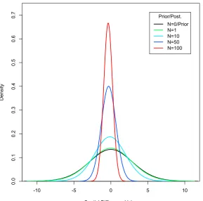
4.2. Comparisons of Student T distributions . . . 46

4.3. Bayesian sequential learning whenσe is unknown . . . 47

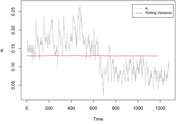
4.4. Spatial difference sensor data ei with its mean adjusted rolling vari-ance. . . 53

4.5. Time varying weights with ψ = 0.1 (top) and ψ = 0.3 (bottom) respectively. When ψ is larger, more weight is given to recent obser-vations, and vice versa . . . 56

4.6. An overview of the message passing sequence. . . 57

4.7. A WSN deployment with spatial fault detection . . . 60

4.8. Memory footprint of the solution versus the number of local spatial models . . . 62

4.9. Time varying model update . . . 66

5.1. The intra-node attributes correlation: humidity versus temperature . 73 5.2. The learnt bivariate Gaussian surface and contour plots . . . 76

5.3. Data fault test via conditional Gaussian distribution . . . 79

5.5. Hierarchical fault detection procedure . . . 82

5.6. Overhead analysis of SDV and HDV . . . 89

5.7. Sensitivity & specificity of HDV and SDV . . . 94

5.8. Finding sensor faults in real data . . . 95

5.9. Comparison with PLA . . . 96

5.10. The adaptiveness of HDV . . . 98

5.11. The effect of time varying parameter estimation . . . 98

6.1. Tree based routing and how TAG saves energy by schedule manage-ment. . . 107

6.2. LEACH data collection based on clustering. . . 109

7.1. Directed graph of a typical HMM . . . 114

7.2. Transition probability matrix estimation . . . 124

7.3. Data collection procedures with HMM . . . 126

7.4. Data collection with HMM with various precisions . . . 131

7.5. The trade-off between accuracy and data compression rates. . . 132

7.6. Applying the HMM solution to real world sensor data with real data faults. . . 133

7.7. Clustering decomposition of the Intel Lab sensor nodes . . . 137

7.8. Cooperative data collection procedures . . . 138

8.1. Dynamical linear model based data collection framework flow chart . 148 8.2. DLM-based forecast and its confidence interval . . . 149

8.3. Evaluation of the DLM-based solution on Temperature sensor data. . 153

List of Tables

2.1. Current consumption for different operations of sensor nodes (adapted

from [2, 3, 4, 5]) . . . 12

2.2. Current consumption for different operations of sensor Nodes [2] . . . 14

4.1. A summary of parameters for spatial correlation based fault detection 61 4.2. Program size comparison . . . 62

4.3. Different fault models . . . 63

4.4. Simulation results of detection accuracy . . . 65

4.5. Comparing with PLA . . . 65

5.1. Model variables used in the overhead analysis . . . 86

5.2. Program sizes of local fault detector and hierarchical physical model fault detector . . . 90

5.3. A summary of parameters for fault detection with local bivaraite Gaussian model . . . 91

5.4. Simulation results of detection accuracy for SDV . . . 92

5.5. Simulation results of detection accuracy for HDV . . . 92

5.6. Evaluation of the robust learning algorithm . . . 96

5.7. Robust learning effect . . . 97

7.1. Evaluation of the proposed data collection method with HMM on Temperature Sensor . . . 129

7.2. Evaluation of the proposed data collection method with HMM on Voltage readings . . . 130

7.3. Evaluation of the proposed data collection method with HMM on Humidity sensor . . . 130

7.4. Fault detection accuracy evaluation of the proposed data collection method . . . 134

8.1. A summary of parameters for DLM based data collection . . . 151

8.2. Simulation results on temperature sensor data . . . 155

8.3. Simulation results on humidity sensor data . . . 156

Acknowledgements

First, I would like to thank my supervisor, Prof. Simon Dobson. He not only pro-vided me with invaluable advice and guidance on my research, but he also shared his life experience with us. I have learnt so much from him, from finding research interest to learning how to do research, from sensor techniques to all sorts of knowl-edge and stories he shared with us. His constant support and belief in me gave me the courage to finish my Ph.D.

I am thankful for my second supervisor Dr. Dharini Balasuhramaniam and my reviewer Dr. Adam Barker. Their suggestions and advice on my research are always helpful. I am thankful for Dr. Juan Ye, Saray Shai, Yi Yu, Chonlatee Khorakhun, Dr. Derek Wang, Masih Hajiarabderkani and Chris Schneider. Many research ideas were spurred during the discussion with them. I also need to thank the Institute of Mathematics and Statistics at St Andrews, where I sit in many lectures without being charged. I would love to thank my teammates at St Andrews Men’s Volleyball Team. Playing with them makes my life physically healthier and more joyful. I thank Dr. Danny Hughes with whom I did two month internship in China.

I thank my parents for their love and support throughout my growing up, and my elder brother for his encouragement. They have provided as much as possible to ensure that I have a good education. Without them, I could have never started my study abroad.

Wireless Sensor Networks (WSNs) form a new paradigm of computing that allows the physical world to be measured at an unprecedented resolution; and the impor-tance of the technology has been increasingly recognised. However, WSNs are still facing critical challenges, including the low data quality and high energy consump-tion. In this thesis, formal statistical models are employed to address these two practical problems. With the formalism that is properly designed, sound statistical inferences can be made to guide local sensor nodes to make reasonable and timely decisions at local level in the face of uncertainties.

To improve data reliability, we introduce formal Bayesian statistical method to form two on-line in-network fault detectors. The two detection techniques are well integrated with existing data collection protocols. Experimental results demonstrate the technique has good detection accuracy but limited computational and commu-nication overhead.

List of Publications

Some of the work presented in this thesis has been previously published:

• Lei Fang and Simon Dobson. Data collection with in-network fault detection based on spatial correlation. In Proceedings of the 2nd International Con-ference on Cloud and Autonomic Computing (CAC 2014), CAC ’14. IEEE,

2014

• Lei Fang, Simon Dobson, and Danny Hudges. An error-free data collection method exploiting hierarchical physical models of wireless sensor networks. In Proceedings of the 10th ACM Symposium on Performance Evaluation of Wireless Ad Hoc, Sensor, & Ubiquitous Networks, PE-WASUN ’13, pages 81–

88, New York, NY, USA, 2013. ACM

• Lei Fang and Simon Dobson. Unifying sensor fault detection with energy con-servation. InProceedings of the 7th International Workshop on Self-Organizing Systems, IWSOS ’13. Springer, 2013

• Lei Fang and Simon Dobson. In-network sensor data modelling methods for fault detection. In Evolving Ambient Intelligence, pages 176–189. Springer,

2013

• Lei Fang and Simon Dobson. Towards self-management in WSNs by exploit-ing statistical model. Poster presented at 6th International Workshop on Self-organizing Systems, IWSOS’12, TU Delft, the Netherlands, 2012. Best Stu-dent Poster

In submission:

• Lei Fang and Simon Dobson. Fault detection based on hierarchical physical models: a Bayesian approach. Manuscript submitted for publication (2014)

• Lei Fang and Simon Dobson. Combining adaptive sampling and energy effi-cient data collection with Dynamic Linear Models. Manuscript submitted for publication (2014)

Others:

• Klaas Thoelen, Danny Hughes, Nelson Matthys, Lei Fang, Simon Dobson, Yizhou Qiang, Wei Bai, Ka Lok Man, Sheng-Uei Guan, Davy Preuveneers, et al. A reconfigurable component model with semantic type system for dynamic wsn applications. Journal of Internet Services and Applications,

Part I.

Introduction

Technological advances in microelectromechanical system (MEMS), wireless commu-nication, and digital electronics, have paved the way for the rise of a new generation of computing networks: wireless sensor networks (WSNs). A wireless sensor network consists of sensor nodes with wireless communication capabilities deployed over a geographical region to monitor some physical process. The importance of WSNs has been widely recognized: WSNs have found their ways in various working scenarios from military battle field to indoor households, from construction sites to human body. The benefits brought by WSNs are all-around.

The reasons that contribute to the success of WSNs can be summarized as follows. First, WSN is an economic choice comparing with traditional monitoring options. Sensor nodes are much cheaper than general purpose computers and human re-source. Second, WSNs provide unintrusive monitoring such that the impact on the environment is minimised. Last but not the least, WSNs provide measurements at unprecedented spatial and temporal resolution. Using dense deployment and sam-pling, the monitoring area of various sizes can be covered. More importantly, sensors can reach places where traditional methods cannot be used. The most important example is hazard monitoring in which floods, volcano eruptions, and earthquakes are monitored.

1.1. Motivation and Challenges

Chapter 1. Introduction

and environmental science. From the data user side, in the current era of Big Data, how to make sense of the data, and furthermore, based on which how to adaptively deploy and sense the environment is a question which requires joint efforts from both sensor community and data scientists.

In this thesis, we focus more on how data is sampled and collected at local sensor level. More specifically, two practical problems are addressed: data reliability and energy management. The first question is raised because of the poor data quality

of WSNs: significant number of sensor data faults have been found in real world WSN deployments [11, 12]. Unreliable sensors have seriously hindered the further utilization of the technology in scientific and critical systems. Therefore, the first problem this thesis aims at is to design algorithms to improve data reliability for WSNs. The second question concerns energy. Sensor nodes are battery-powered

and expected to operate autonomously in rural areas. Longevity is critical to the application: sensors may not be harvested after deployment, and short lifetime means huge waste. Therefore, the second question this thesis addresses is how to collect data in an energy efficient way.

However, due to its unique physical nature, WSN research faces serious challenges or difficulties.

Resource-constrained: The limited resource here refers to incapable computing ca-pability, small storage, and limited energy budget. The three insufficiencies cause trouble especially in algorithm and protocol design: the proposed solu-tion should be within the feasible computasolu-tional capacity of sensor nodes and have limited energy expenditure.

Highly distributed: The distributed nature makes any centralised control design inappropriate, as it not only increases overall network communication but compromises scalability.

1.2. Uncertainty and Statistical Models

1.2.1. Ubiquitous Uncertainty

For WSNs, uncertainties are everywhere. First, the physical world that WSNs mea-sure is uncertain. Actually, the lack of knowledge on the evolving but uncertain

physical process is the main driver behind most WSN deployments. Deterministic process will be of little interest to WSNs, as a deterministic mathematical model or even a complete enumeration of the quantity of interest is sufficient. For example, by the energy conservation law, the movement of a pendulum under certain per-fect conditions (like in a vacuum space with no air resistance, no friction with the

attached string and so on) can be completely quantified by a simple period equation

T = 2π

s

L

g, (1.1)

where L is the length of the pendulum, g is the the acceleration of gravity, and T

is the period [13]. However, “perfect conditions” are fairy tales that rarely exist in reality. Even for this trivial experiment, thereal period is stilluncertain.

Second, WSNs only hold a partial view of the physical world. For a deployment, no matter how densely the nodes are deployed or how frequent the nodes are missing. To give an extreme example, future observations can never be concretely measured. They are completely “uncertain”, and can only be “guessed”.

Third, sensor measurements themselves are uncertain. They are at best the noisy version of the reality. Indeed,uncertainty is everywhere.

1.2.2. Dealing with Uncertainty

Quantifying the above uncertainties becomes crucial to understanding the under-lying physical process and to perform WSNs control. As suggested by Berliner, complex uncertainty “naturally leads to the use of random or probabilistic meth-ods” [14]. Statistical modelling that makes great use of probabilistic methods be-comes a promising tool to deal with the uncertainty. Statistical modelling is a broad concept which encompasses all mathematical modelling methods that employ prob-ability distributions to solve their problems [15]. The key feature of a statistical

model is the use of probability distributions to quantify variability.

Take the pendulum case as an example again, the period,T, is no longer a certain

Chapter 1. Introduction

of having a constant truth value, its value now varies according to a distribution. Based on the distribution, you may still obtain a point estimate by calculating the most probable estimate (with the largest probability). But a better estimate would be an estimation interval associated with a probability confidence. Based on the distribution, we may ask more interesting questions like what the future period would be given what has been observed so far, and how certain that prediction is; or after an outrageous observation is taken, how likely that measurement is a fault. Answering such questions based on the distribution, or equivalently the statistical model, is calledinference.

This thesis advocates the idea of using statistical models for uncertainty man-agement in the field of WSNs. We employ formal statistical models to quantify uncertain sensor measurements. And based on the data model and inference tools, local sensors can automatically make timely but informed decisions. This approach that purely relies on sensor data rather than human intervention or expert knowledge is a data centric approach.

1.3. Thesis Objectives and Contributions

The main thesis objective is to demonstrate:

• Statistical methods can be used to solve practical sensor problems in a realistic way even given the challenges faced by WSN platform. Note that an important message the statement tries to convey is that statistical modelling that provides formal reasoning and inference is not only useful but also can be deployed at sensor node level. The main contributions of this thesis are as follows:

• A distributed and on-line fault detection method capable of filtering out faults in real-time by making use of spatial correlation and formal Bayesian analysis. The fault detection method is also well integrated with existing data collection protocol. (Chapter 4).

• A novel data collection framework which employs Hidden Markov Model to energy efficiently gather error-free data. The solution is an unified solution that improves data reliability while achieves energy conservation. A spatial-coherence-aware extension based on the HMM solution is studied to provide an alternative to the traditional cooperative sensing technique. (Chapter 7)

• A Dynamical Linear Model (DLM) based data collection framework featuring both adaptive sampling and energy efficient data collection. (Chapter 8)

Different statistical models of increasing complexity and expressive power are used from Chapter 4 to Chapter 8. Such a waterfall illustration is adopted to show the power of statistical modelling as well as the rich functions served by the different models.

1.4. Thesis Structure

The presentation of the thesis generally follow a problem solving approach. Part I introduce basic backgrounds on WSNs and statistical modelling.

• Chapter 2 introduces backgrounds on WSNs and statistical models. Important features of sensor data are presented as well as statistical modelling basics.

Part II is dedicated to the research question of data reliability.

• Chapter 3 gives an general introduction of sensor fault detectors. The impor-tance of on-line and in-network detection is stressed. The state of art and related works on sensor fault detection are surveyed.

• Chapter 4 introduces the first contribution of this thesis: a spatial correlation based fault detector. The solution follows a formal Bayesian approach.

• Chapter 5 introduces another fault detector that exploits two layers of phys-ical models. The new method has smaller communication overhead but has comparable detection performance.

Part III concentrates on energy efficient data collection methods.

Chapter 1. Introduction

• Chapter 7 presents a novel data collection method featuring the application of HMM. An extension that makes use of both spatial and temporal correlations is studied. In terms of statistical modelling, HMM is a richer model than the simple structured models used in Part II.

• Chapter 8 presents the final contribution of this thesis: a Dynamical Linear Model based data collection framework. Regarding the employed model, DLM can be viewed as an extension to HMM.

Finally, Chapter 9 in Part IV concludes the thesis and gives future work directions.

1.5. Notations

Throughout this thesis, the following notations are used. Boldface is reserved for vectors, and normal font refers to scalars. Theorems, Lemmas and Propositions in the thesis are findings worked out and proved by the author; while Results are reserved for existing knowledge or findings from others’ works.

Abbreviations and acronyms

R.H.S Right hand side of an equation L.H.S Left hand side of an equation FI Fisher information metric OLS Ordinary least square

t.p.m Transition probability matrix p.d.f Probability density function

iid independently and identically distributed GMM Gaussian mixture model

G-HMM Gaussian Hidden Markov model WSN Wireless sensor network

WSAN Wireless sensor and actuor network HMM Hidden Markov model

DLM Dynamic linear model CPU Central processor unit MCU Microcontrollor

RF Radio frequency

MLE Maximum likelihood estimator MAP Maximum a posteriori estimator

ARIMA Autoregressive integrated moving average model AR Autoregressive model

HBST Hierarchical Bayesian space-time model MCMC Markov chain Monte Carlo

TP True positive FP False positive TN True negative FN False negative

Mathematical Notations

P(ω) Probability of event ω, in the range of [0,1]

p(X) Probability density function for the random variable X

P(A|B), p(A|B) Conditional probability (density) of A given B Xt Sensor measurement sampled at time t

X(t) _{Measurement collection {X}

1, . . . , Xt}

E[X] Expectation of a random variable X

Var[X] Variance of a random variable X

Cov[X, Y] Covariance of two random variables X and Y

D Data set; sensor series data N(µ, σ) Gaussian distribution

T(a, b, c) Student T distribution

N G(m, n, a, b) Normal Gamma distribution

Chapter 2.

Background

2.1. Wireless Sensor Networks

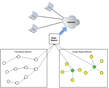
Wireless Sensor Networks are typically formed from multiple battery-powered sensor nodes, interconnected with short range wireless communication channel, like RF (radio frequency), measuring and reporting real-world quantities through one or more powerful gateway “sink” nodes which have accesses to infrastructured networks like Internet. Figure 2.1 shows this operation graphically. In Figure 2.1, two WSNs of different network topologies are shown: the first one is a flat network where sensor data is relayed to the sink via tree-like routing paths; the other is a cluster-based topology, where the cluster heads collect data from the member nodes and communicate with the sink.

Note that there are other specialised types of sensor networks, like Wireless Sensor and Actuator networks (WSANs) [16, 17], Video Sensor Networks (VSNs) [18, 19], or more general Multimedia Sensor Networks (MSNs) [20] which are not the focus in this thesis. The thesis targets at more general sensor networks where the sensor nodes are more resource constrained.

Figure 2.1.: Data gathering of a WSN deployment with a gateway to Internet. The left WSN is a flat network and data is collected by a routing tree towards the sink; the right is a hierarchical structure where the green nodes are cluster heads and the yellow nodes are cluster members.

2.1.1. Sensor Node

In this section, we study WSNs at a lower level: sensor nodes, the building blocks of a WSN. As a basic unit of WSNs, a typical sensor node, also called mote, should be able to perform the following principal tasks – computation, sensing, communication and storage. The tasks are donevia five constituting hardware components (see

Fig-ure 2.3): controller, sensor, memory, communication and power supply. Table 2.1 lists four types of sensor nodes together with their essential hardware specifications.

Controller

Sensor nodes need to perform processing tasks ranging from time-critical signal pro-cessing, communication protocol processing to local application programs. These tasks cannot be done without a processing unit, called a microcontroller (MCU),

Chapter 2. Background

Figure 2.2.: A classification of WSN applications (adapted from [21]).

Table 2.1.: Current consumption for different operations of sensor nodes (adapted from [2, 3, 4, 5])

Mica2 MicaZ Telos TelosB

Producer Crossbow Crossbow Imote iv Imote iv

MCU Atmel Atmega

128L Atmel Atmega128L MSP430 MSP430

Speed (MHz) 7.4 7.4 8 8

RAM (KB) 4 4 2 10

ROM (KB) 128 128 60 48

Radio Chipcon

CC1000 ChipconCC1000 ChipconCC2420 ChipconCC2420 Max Range 150-300 m 75-100 m 75-100 m 75-100 m

Data Rate 38.4 (kbps) 38.4 (kbps) 250 (kbps) 250 (kbps) Power 2 AA batteries 2 AA batteries 2 AA batteries 2 AA batteries

in embedded systems where energy efficiency is a critical concern [31]. Commonly used MCUs for sensor motes include Atmel Atmega 128L for Mica node family, and MSP430 for Telos nodes.

Sensors

Sensor is the defining component of a sensor mote, which is a hardware device that produces a measurable response signal to a change in a physical condition such as temperature, humidity, and light [32]. Over thousands of sensors have been invented to measure quantities like temperature, pressure, humidity, acceleration, light and so on. New types of sensors like chemical and biosensors are also emerging for more complex environmental proxies in situ measurement [33]. Note that a mote can

integrate in more than one type of sensor.

Memory

Chapter 2. Background

sensor data are processed in an on-line fashion and no large volume local storage is necessary. Some nodes offer external flash memory in addition to the on-chip storage to compensate for the limit internal space. However, the long access delay of flash as well as the associated energy consumption rate should not be ignored [31]. Therefore, frequent or intensive flash access should be avoided.

Communication

The communication component is responsible for exchanging data between individ-ual nodes. Among those available wireless transmission media, Radio Frequency (RF)-based communication is by far the most popular and relevant one. RF-based communication provides relative long range and high data rate transmission at rea-sonable energy expenditure, which makes it suitable for sensor notes.

Power

The most common power source for sensor nodes are batteries. Three types of battery technologies can be used in WSNs, i.e. alkaline, lithium and nickel metal hydride [34]. The three materials have their own merits as a power source for motes. For example, alkaline is a cheap but high-capacity energy source, and lithium batteries are of smaller size. Power scarcity is a big problem facing WSNs as fetching and replacing flat batteries is generally infeasible. Noticeably, some new technologies that enable energy harvesting have been proposed [35].

2.1.2. Energy Efficiency

Power is the most valuable resource for WSNs as it determines the lifetime of the deployment. For WSNs deployed in rural area or hazardous region, the deployment is expected to last as long as possible without human intervention. To achieve this goal, advances in hardware technology, like better battery design or solar power harvesting, certainly are important. However, effort from the hardware side alone cannot solve the problem completely. It is the sensor software that ultimately de-termines how the energy is spent. Therefore, energy efficient software clearly should be given more attention. The state of art on energy efficient software is presented in Section 6.2.

operations consume more energy than the others. The energy cost for ROM, or flash, access cannot be overlooked neither. The ratio of the energy consumption to send one bit compared to computing a single instruction ranges from 190 to 2900 for different hardware platforms [31, 36, 37]. Pottie and Kaiser [38] provides the com-parison from another perspective: communicating 1 KB of data over 100m consumes roughly the energy that is equivalent to the amount spent in computing three million instructions. Therefore, it is usually assumed that computation without accessing flash memory is significantly cheaper than radio communication.

Table 2.2.: Current consumption for different operations of sensor Nodes [2]

Operation Mode Mica2 MicaZ TelosB

Standby 19.0 µA 27.0µA 5.1 µA

MCU Idle 3.2 mA 3.2mA 54.5 µA

MCU Active 8.0 mA 8.0mA 1.8 mA

MCU + Radio RX 15.1 mA 23.3 mA 21.8mA

MCU + Radio TX 25.4 mA 21.0 mA 19.5 mA

MCU + Flash Read 9.6 mA 9.4mA 4.1 mA

MCU + Flash Write 21.6 mA 21.6 mA 15.1 mA

2.2. Sensor Data

In this section, a detailed study on sensor data is presented. Firstly, important sen-sor data features including multidimensionality, non-stationarity, spatio-temporal correlation, are discussed in detail. The illustration is accompanied with examples taken from real world sensor data. Next, sensor data faults are introduced. We first give the definition of sensor data fault; a taxonomy of the faults is presented after the possible roots of the faults are explored.

2.2.1. Sensor Data Features

Multi-dimensionality

ensem-Chapter 2. Background

ble form multivariate time series. Figure 2.4 shows sensor readings of temperature, humidity, light and voltage collected from a deployed node in Intel deployment [1].

18

20

22

24

26

T

emp

era

tu

re

25

30

35

40

H

umi

di

ty

0

100

300

500

Light

2.62

2.66

2.70

2.74

0 1000 2000 3000 4000 5000

Vo

lta

ge

Time

Figure 2.4.: Four types of sensor readings collected by one node of Intel deploy-ment [1]

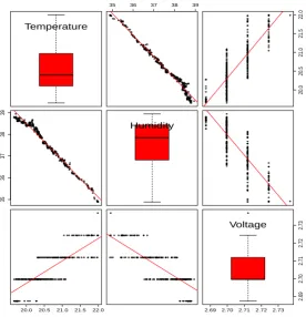
The multi-variate nature of sensor readings bring both benefits and difficulties with regard to sensor data modelling. The different classes of sensor readings tend to be correlated and such local correlations can be exploited to find outlier data entries in an energy efficient way as no inter-node data transmission is required. For example, the readings of humidity and barometric pressure sensors are related to the readings of the temperature sensors [39]. Figure 2.5 shows the mutual correlations between temperature, humidity, and voltage.

Temperature

35 36 37 38 39

20.0

20.5

21.0

21.5

22.0

35

36

37

38

39

Humidity

20.0 20.5 21.0 21.5 22.0 2.69 2.70 2.71 2.72 2.73

2.69

2.70

2.71

2.72

2.73

Voltage

Figure 2.5.: The linear correlations among sensor data

−8 −6 −4 −2 0 2 4

−4

0

2

4

6

8

Variable X

V

ar

iab

le Y

outlier

Figure 2.6.: An example of bivariate outlier

Chapter 2. Background

Non-stationarity of Sensor Data

Stationarity is an important concept in statistical time series analysis. Roughly speaking, a data series is stationary if its behaviour is self-similar therefore its sta-tistical properties, like the mean and variance, do not vary over time. This assump-tion is generally not realistic for most real world data, but it greatly simplifies the mathematical model for the data as well as the computation [41].

For WSNs, this assumption bears a fundamental loophole: if the phenomena of interest were truly stationary, there would be no need to deploy sensors to moni-tor the phenomena whatsoever as the whole underlying process remained constant. Sensor data are inherently non-stationary. As shown in Figure 2.4, the temperature readings, for example, change radically along the time stamps. In terms of data modelling, non-stationarity brings serious modelling difficulty: as any model learnt by historic data will turn stale at some stage.

Correlation of Sensor Data

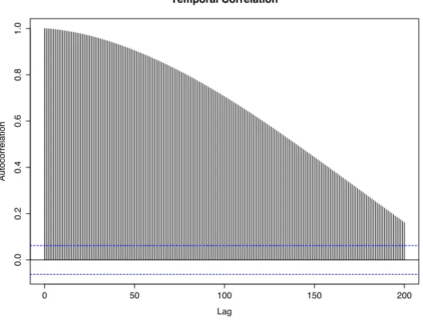
Due to the fact that the underlying phenomenon usually is dominated by a smooth continuous process, sensor data tend to be correlated in both time (temporal corre-lation) and space (spatial correcorre-lation).

0 50 100 150 200

0.0

0.2

0.4

0.6

0.8

1.0

Lag

Autocorrelation

Temporal Correlation

Figure 2.7.: The autocorrelation of temperature sensor data

Time

T

emp

era

tu

re

°

C

0 2000 4000 6000 8000 10000 12000 14000

16

18

20

22

24

26

28

Node 2 Node 3 Node 33

Node 34

Figure 2.8.: Time series plot of spatially co-located sensor nodes

the underlying physical process is continuous and the sampling frequencies adopted by sensors nodes are high enough to capture this smoothness. Fig-ure 2.7 shows the autocorrelation of temperature sensor data from the Intel

deployment [1]. Sample autocorrelation measures the self-similarities within a time series. Its value ranges from −1 to 1. And the closer the absolute value

of the estimate to 1, the stronger is the correlation between them. It is evident from the figure that the data with shorter lag differences tends to be stronger correlated.

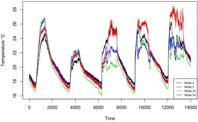
Spatial Correlation Spatial correlation implies that sensor data from geographically close nodes are expected to be similar [42]. This assumption is true for WSNs because the node-to-node distances (less 200m) are close (therefore, they are

almost measuring the same phenomena). Figure 2.8 shows spatial correlations among adjacent nodes from the Intel data [1].

2.2.2. Sensor Data Faults

Garbage In Garbage Out (GIGO), is a notion in computer science mainly referring

Chapter 2. Background

produced by wireless sensors networks (WSNs).

By retrospecting some successful WSN applications, it has been found that a substantial portion of the data gathered in real world WSN deployments is actu-ally garbage. For example, 51% of the data collected in [22] was faulty; 3-60 % of

data collected in the Great Duck Island experiment was incorrect [43]. Other data series [1, 44] also have been found faulty. However, for the users of WSNs, rang-ing from scientific exploration [22], to infrastructure protection [25], most of which demand highly accurate data input. The low reliability associated with sensors, therefore, has become the main factor that prevents the further commercialisation of WSN technology.

The Causes of Data Faults

Sensor data faults emerge when a node performs, or is forced to perform, a sensing

task in an erroneous way resulting in faulty data which deviates from a true sample of the physical context to be measured. Data-faults in general are generated by internal (i.e. system faults) or external factors. External source usually involves various kinds of malicious attacks, like unauthorised message spoof or node tam-pering [45], which lead to the received data altered. Intrusion detection or sensor network security [45], [46], [47], are the researches that deal with these external factor. On the other side, internal sources include battery failure, weakening bat-tery supply, connection failure, sensor hardware malfunctioning, calibration error, short-circuited connections and so on [11, 12].

Data Outliers

Data Faults

Internal External

Event Outliers

Battery Failure

Connection Failure

Sensor Failure

Message spoof

Node tamper-ing

Unexpected Events (vol-cano eruption etc.)

Figure 2.9.: The relationships between data-outlier and data-fault and their sources.

Data Fault Types

Sensor data faults can be categorised into five categories, i.e. noise, short, constant, calibration and jump. According to [11, 12], the fault types have been constantly found in different WSNs deployments [22, 1, 44, 48, 49]. The definitions of the five categories of faults are listed below. Figure 2.10 presents examples of the sensor faults found in a deployment [1].

NOISE Sensor readings exhibit an unexpectedly high amount of variation for a period of time. The noisy variance is beyond the expected variation of the underlying phenomenon. Usually high noise is due to a hardware failure or low batteries [11].

SHORT A sharp momentary change in the measured value between normal con-secutive readings. Hardware failures like fault in the analog-to-digital convert board may lead to short faults [12].

CONSTANT Also known as “Stuck-at” fault. The readings remain constant for a period of time greater than expected. The reported constant value usually is out of the possible range of the expected normal readings and uncorrelated to the underlying physical phenomena [12].

Chapter 2. Background

time

time

time

time

Figure 2.10.: The four types of sensor data faults: Noise, Short, Jump and Constant respectively found from the Intel deployment (Note Calibration fault is hard to display graphically without ground truth) [1].

2.3. Statistical Modelling

In this section, preliminaries on statistical modelling are presented. First, we give a general statistical model for a temporal process. Next, we show how the model can be used to draw conclusion, i.e. make inference. An important school of statis-tics, Bayesian method, is introduced afterwards. The Bayesian method and Bayes’ theorem are intensively used in the rest of the thesis. Last, general components of statistical modelling are discussed.

2.3.1. Statistical Models

Sensor data, in essence, is a collection of time series, or series of observations taken sequentially in time. In this section, we present a general formalism to model time series data. First, an important concept calledstochastic process is introduced.

Definition 2.1 (Stochastic Process). A stochastic process is a collection of ran-dom variables

{X(t) :t ∈Dt.} (2.1)

1. We call {X}acontinuous-time process ifDtis a uncountable interval, such as Dt = [a, b], or [a,∞) with a < b.

2. We call {X} a discrete-time process if Dt is a finite or countably infinite set, such as Dt={0,1,2, ...}.

3. The joint probability distribution associated with the random vector of {X}, denoted as p({X}) or p(X0, X1, X2, ...) for the discrete process case, is called

the finite dimensional distribution.

4. A sequence of samples, x= (x0, x1, x2, ...)

0

, generated according to the finite

di-mensional distribution, is called a realizationorsample pathof the process {X}.

For sensor data collected at a fixed frequency, it can be modelled by a vector of

T random variables, which can be written as

{Y(t) :t∈T}, (2.2)

where t indexes the time of the measurement. Therefore, by Definition 2.1, the

Chapter 2. Background

a collected sensor data series is simply asample path of the stochastic process. For

the sake of simplicity, we will use process directly instead of stochastic process in the rest of the thesis.

Note the flexibility of the process model. We can modify it slightly to model multivariate sensor data as well as spatially correlated sensor data. For example, when each Yt, t = 0,1,2, ... is a k × 1 random vector such that Y(t,i) : 1 ≤ i ≤

k represent different variates, say temperature, humidity, light, and voltage, then

{Yt : t ∈T} is a multivariate stochastic process. A spatial process can be obtained

by definingDt as a subset of R2 to represent a two dimensional geographical space.

2.3.2. Making Inference

Drawing conclusions based on a probability model is called inference. The finite dimensional distribution of a process, p({Yt :t = 0, ..., T}) defined in Definition 2.1,

provides us the complete information about the variation of the process. The fol-lowing two results show that how the distribution can be manipulated to form new distribution such that more specific inferences can be made.

Result 2.1 (Marginal Distribution). For any index subset S ⊆ T, define its

com-plement as ¯S =T \S,

p({Yt:t∈S}) =

Z

¯

S

p({Yt:t∈T})d{Yt:t∈S¯}. (2.3)

Result 2.2 (Conditional Distribution). For any disjoint index subsets R, S ⊆ T,

and R∩S =∅,

p({Yt:t ∈R}|{Yt:t ∈S}) =

p({Yt :t∈R∪S})

p({Yt:t ∈S})

. (2.4)

By marginalization (Result 2.1), we can obtain a marginal distribution of any subset of the random vector that are of particular interest. For example, if the sen-sor measurement at t = 10 is of interest, we can obtain a marginal distribution on Y10 itself by integrating out the rest by Equation (2.3). More informed conditional

probability distributions can also be formed based on the joint and marginal distri-bution by Result 2.2. For example, if we are interested in future measurement ats

and we have already observed measurements up tos−1, we can calculate the

probability distribution:

P(a ≤Ys≤b|{Yt, t∈ {0, . . . , s−1}}) =

Z b

a

p(Ys|{Yt, t∈ {0, . . . , s−1}})dYs, (2.5)

where the conditional distribution is calculated according to Equation (2.4) by let-ting R ={s} and S ={0, . . . , s−1}. This is an example of making inference, and

the subject of the inference is the future measurementYs.

Last, to make the illustration complete, we give the definitions for expectation, variance, covariance and correlation, which summarize statistical features

of/be-tween random variables.

Definition 2.2 (Expectation, (Co)variance, and Correlation). Recall the expected value of a function over a random variable is defined by

E[f] =

Z

p(x)f(x)dx. (2.6)

The mean and variance of a random variable X, the covariance, and correlation between two random variables X, Y are defined respectively by,

µX =E[X], σ2X = Var[X] = Cov[X, X]

Cov[X, Y] =E[(X−µX)(Y −µY)], Cor[X, Y] =

Cov[X, Y] σxσy

Mean and variance are also called the first and second moments of a random variable. They measure the location and spread of the distribution of a random variable respectively. Covariance, on the other hand, measures the relationship between two random variables. Positive covariance means two random variables are positively correlated (greater values of one variable are associated with the greater values of the other), and vice versa for negative covariance. Correlation is the

standardised covariance whose value ranges from -1 to 1.

2.3.3. Model Learning

Bayesian Method

Chapter 2. Background

Assume we have data set D, a statistical model h with model parameter θ.

Ac-cording to Bayes’ theorem,

p(θ|D, h) = p(D|θ, h)p(θ|h)

p(D|h) . (2.7)

Sincep(D|h) does not depend on θ, Equation (2.7) can also be written as:

p(θ|D, h)

| {z }

posterior

∝p(D|θ, h)

| {z }

likelihood

p(θ|h)

| {z }

prior

. (2.8)

Note the Bayesian approach treats the unknown model parameter θ as a random

variable with the associated prior and posterior distributions. Theposterior is the conditional distribution of the model parameter given the data. Bayes’ theorem allow us to calculate the posterior as the product of likelihood (given a concrete model, the probability of observing the dataD) and prior (parameter distribution before the data is observed).

The posterior distribution can be used to predict future observations. The dis-tribution of unseen data given what has been (partially) observed, D, is called predictive distribution: p(dnew|D), which can be calculated as follows:

p(dnew|D) =

Z

p(dnew, θ|D)dθ (2.9)

=Z p(dnew|θ,D)p(θ|D)dθ. (2.10)

An interpretation of this formula is that the updated belief (posterior) is used to predict future observation by averaging all possibilities of θ which are weighted

according to the posterior.

Likelihood & Maximum Likelihood Estimate

According to Equation (2.8), the likelihood term is defined as

L(θ) =p(D|θ, h),

i.e. the probability of observing a data setDconditional on the model parameter θ.

When the learning data D is fixed (they are concrete observations), the likelihood

can be viewed as a function ofθ: different parameters will give different likelihood.

By maximizing this function, we can find the estimator ˆθ such that the likelihood

estimator (MLE). The MLEs therefore are the parameters that best explain the data. Depending on the model, some likelihood function can be optimized analytically, like the linear regression model, which lead to closed form maximum likelihood estimators. However, for most problems of non-linear or complex structures, an iterative expensive Gradient-based optimizer is needed to find the MLEs [51].

2.3.4. Modelling Steps

A typical statistical model based solution is formed by the following four compo-nents. The procedure starts with a model assumption step, in which the problem is abstracted into a probability model; a parameters learning step, in which the model is fully specified with learnt parameters supplied; a problem solving stage, i.e. the model is put into use; and a model update component, which adapts the model, typically the parameters, to the changing physical world.

Model Assumption Based on the feature of the problem, a statistical model is de-veloped. The model typically specifies the dependence relationships between the modelling random variables (dependence structure) and also the mod-elling parameters. For example, Gaussian random variables are usually used to model real valued quantities, like temperature, the mean vector and variance-covariance matrix are the parameters. The model complexity depends on the nature of the problem as well as the modelling data.

Parameter Estimation The parameters of the statistical models are estimated ac-cording to certain criteria, like maximum likelihood (MLE), minimum-variance unbiased estimators (MVUE) or even heuristically by field knowledge or rea-sonable assumption.

Problem Solving via Inference The constructed model with estimated parameters are put into use to solve problems. For example, for fault detection problem, the model can answer whether and how likely a new observed sensor reading is a fault.

Chapter 2. Background

2.3.5. Why Statistical Methods ?

In this thesis, different models of various levels of complexity are used. For example, to form fault detection, a statistical model with simplified dependence structure is used to model the spatial sensor data. The simplified dependence structure brings in the benefit of computational convenience but also meets the application’s require-ment (detecting data fault). On the other hand, to forecast future data readings, more powerful models are required. To make the forecasting informative and accu-rate, Chapters 7 and 8 enriches the model by employing sophisticated time series models that introduce an additional latent process to the observational temporal process. Therefore, the choice of the model is problem dependent.

The reasons statistical methods are put forward can be summarized by the fol-lowing arguments.

Resolves uncertainty As discussed in Section 1.2, sensor applications involve dif-ferent forms of uncertainties. For example, for data fault detection problem, whether a data entry is a genuine fault or a false alarm is uncertain. Effectively managing these uncertainties is critical to a WSN application. Therefore, sta-tistical methods that employ stasta-tistical models to quantify those uncertainties are a natural choice.

Sound inference Statistical methods make formal and sound inferences possible. For example, by using a credible interval for a sensor reading, informed de-cisions can be made such as how likely that reading is a fault or vice versa. Comparing withad hocmethods which relies heavily on human intervention or

expert knowledge, statistical methods are more suitable for sensor networks.

Efficiency concern Statistical methods usually are deemed heavy-weight and com-putational intensive; however, it can be shown that with specific assumptions being made, specific learning algorithms, and tailored inference steps being designed, statistical methods can be lightweight, even for WSN nodes. The proposed solutions demonstrate this idea by either real world implementation or formal complexity analysis.

2.4. Summary

In this chapter, background knowledge on Wireless Sensor Networks, sensor data, and statistical modelling is introduced.

In the first section, we present the basics of WSNs. The importance of the tech-nology is revealed by listing its wide range of applications: ranging from military object tracking to day-to-day household health care. The hardware platform of sen-sor motes is further explored in detail. It is learnt that sensen-sor motes have very limited computational capability so is its storage capacity. Any regular compu-tational tasks envisioned for regular computing devices might be overwhelming to sensor motes. Furthermore, energy efficiency is another key problem facing WSNs. All processing, communication and sensing tasks consume energy; and the power supply is limited. How to improve the lifetime of WSNs is crucial to the applicability of the technology. The energy efficiency concern leads to one of the questions that this thesis addresses: For WSNs of monitoring applications, how can we collect data in an energy efficient way?

Secondly, we introduce sensor data. Real world sensor data retain the follow-ing important statistical features, multidimensionality, non-stationarity, and spatio-temporal correlation. These features may complicate the model; but can also be exploited to improve data collection efficiency and quality. Moreover, sensor data is prone to be inaccurate, which severely limits its further application especially in critical systems. The data accuracy concern leads to another problem the thesis tries to address: For WSNs of monitoring applications, how can we improve the data accuracy?

Last but not least, statistical methods are briefly introduced with some important theories and techniques being highlighted. We show statistical methods, by treating uncertainties as random variables, can be used to model sensor data. We further give examples showing how the model can be manipulated and queried to answer questions of practical use. Learning methods: i.e. Bayesian method and likelihood method, are briefly introduced. And last, the key constituent components of a statistical modelling approach: model, parameter learning, inference, and adaptive update are presented.

Part II.

Sensor Fault Detection Algorithms:

An Overview

It has been shown that sensor measurements are prone to be inaccurate. In order to counteract the impacts of garbage containing sensor data, many data-fault-tolerant algorithms have been proposed from the data-user end, especially by the pervasive computing community. For example, several activity and situation recognition algo-rithms that are resilient to uncertain sensor input have been proposed [52], [53], [54]. However, to eradicate the problem, the only choice is to improve data quality of WSNs.

In this chapter, we give an overview to the techniques used to detect sensor faults. First, the desired properties of sensor fault detectors are introduced. The challenges faced by the techniques are listed. Last, we survey the sate of art in the field of sensor fault detection techniques.

3.1. Sensor Fault Detectors

3.1.1. On-line and In-network Fault Detection

Chapter 3. Sensor Fault Detection Algorithms: An Overview

filtering is always an option, we believe on-line and in-network solutions have certain advantages over the traditional method.

• On-line solutions can provide in-time alerts when things go wrong. Therefore, timely remedies can be given, like replacing the faulty sensors, to avoid the collected data set being completely useless.

• In-network solutions are more scalable than their server side counterparts. For large scale deployments, centralised solutions usually causes big overheads.

• In-network solutions are more flexible in that it can operate without sending all the data back to the sink. For some applications, like event driven applications, they do not send row sensor readings back to the sink directly [55].

• Last but not least, the low yield of WSNs applications makes server side error filtering not practical. For example, the Redwood project [22] reported only 49 % of sensor data are finally received, which makes fault detection at sink very challenging, if not impossible.

3.1.2. The Difficulties of Sensor Data Fault Detectors

The design of an on-line in-network solution faces several challenges. First, achiev-ing high detection accuracy is not easy. The faults reported by a detector can be categorised into four classes: data points correctly detected as faulty (true positive); data points correctly detected as non-faulty (true negatives); data points incorrectly detected as faulty (false positives); and data points incorrectly detected as non-faulty (false negatives). Good detection accuracy implies the method should be able to filter out the exactly amount of faulty data, i.e. achieve high true positive rate but keep false negative rate low.

To form an on-line and in-network solution, the technique should be simple enough to be deployed at sensor node level. However, pursuing simplicity of the solution should not compromise its detection accuracy.

Last, for a solution that employs a model, as the learning data to construct the model at the first place is unreliable; therefore, the data modelling method should be

robustto the noisy learning data. Otherwise, a misleading model learnt by erroneous

3.2. Related Works

In this section, the state of art on sensor fault detection techniques is surveyed. Centralised and off-line fault detection solutions are briefly introduced first; and the focus of this survey switches to on-line and in-network solutions in the second half of this section.

3.2.1. Centralised and Off-line Fault Detectors

Fault detectors falling in the centralised and off-line stream are typically applied after the data is collected and right before the real processing or analysis of the data starts. Therefore, any traditional outlier detection methods from data analysis field can be applied here to find data faults. These solutions usually either employ heavy models that are computational infeasible to sensor motes or would cause excessive amount of inter-node communication if they were applied in the network.

Sharma et al. [12] studies data faults, as well as their possible causes. Four

Chapter 3. Sensor Fault Detection Algorithms: An Overview

process can be formed as the sum of a spatial component, a long-term trend compo-nent, a dynamic process accounting for day-to-day variations and a noise component. Some of the components require specific and sound field knowledge as prerequisite. For example, for temperature data, the cyclic period (which is 24 hours usually) is required to specify the long-term trend component. Compared with linear regression models, HBST is significantly more complex but capable of modelling complex phe-nomenon. The model parameters are learnt by Markov chain Monte Carlo (MCMC) method, an expensive and time-unbounded simulation based estimation. Outliers are found by inferring the learnt model. Comparing with other simple models, like autoregressive model, the solution has a similar detection rate but lower false-positive rate. However, apart from the expensive MCMC learning step, the solution only works when the error rate is small, i.e. only a small portion of the sensor data is faulty (otherwise, the faulty data pattern might be learnt as the HBST model), which might not be a valid assumption in WSNs context.

3.2.2. In-network and On-line Fault Detectors

Elnahrawy and Nath [58] employs a Naive Bayesian Classifier to find faulty data. Spatial and temporal correlation, called context information in the work, is modelled by a first-order Markov probabilistic model. More specifically, the solution believes the current sensor reading Xi(t) only depends on (a) the current readings of the

immediate neighbours (spatial correlation), and (b) the last reading of the sensor

(temporal correlation). The solution assumes that the sensor data takes values in the interval [l, u], and discretizes the interval into m mutually exclusive and exhaustive

sub-intervals. The state space is denoted asR={r1, r2, . . . , rm}, where each element

ri represent the statei. Denote the temporal feature as H, and the spatial as S, a

piece of context can be represented as a state tuple, i.e. CI ∈ R×R|S|_{, where |S|}

denotes the size of neighbours.

Based on Baye’s theorem, we can infer the most probable state for the current measurement based on the contextCI. The most probable state is called maximum

a posteriori (MAP) in Bayesian term. The MAP state can be calculated as follows:

rM AP = argmax ri∈R P(

Xi(t)∈ri|H, S)

= argmax

ri∈R

P(H, S|Xi(t)∈ri)P(Xi(t)∈ri)

P(H, S)

= argmax

ri∈R P(

Note (3.1) follows because, for a Naive Bayes classifier, attributes are assumed inde-pendent to each other. In other words, the solution assumes the spatial correlation and temporal correlation are independent. Outliers can be found by comparing the reference resultrM AP inferred from the model and the reality: if they are different,

the measurement is classified as a fault. Simulation results show that the solution has good detection rate to both synthetic data and sensor data. However, the solu-tion has the following limitasolu-tions. First, when the state space is refined, i.e. m is

large, the context information model grows very fast. For example, when n spatial

neighbours are considered, the state space is ofO(mn_{); and whenmornis large, the}

space size is overwhelming to sensor mote’s capacity. Second, the spatio-temporal relationship which is summarized in the Bayesian model is believed to be stable, therefore not updated. This stationary assumption is clearly not valid for sensor data. For instance, in the morning, temperature follows an increasing trend while later in the afternoon it shows a downward trend. Obviously, a morning “context” will not be appropriate for the afternoon data.

Bettencourt et al.[59] propose a solution that exploits both temporal and spatial

correlation. The solution aims at distinguishing events from data faults. In detail, each node learns the statistical distributions of the temporal difference (between its current and previous reading) and spatial differences (between its local reading and neighbours readings). Any data that is significantly deviating from the expected distribution is considered as an outlier. However, the solution does not provide efficient mechanism to update the model.

Non-parametric statistical method based solutions are presented in [60] and [61]. They both use kernel density estimation to learn sensor data distribution. The bene-fit is that no distribution assumption of the sensor data is required. The estimation can provide “customized” distributions for different data patterns (which do not have to be assumed as bell-shaped Gaussian). However, kenel density estimation is known to be computational intensive [62]. Similar solutions include [63], which uses histogram to find outliers. However, the specification of a histogram depends on bin size and bucket width, which are not obvious to specify. Moreover, there is no obvious way to update the histogram such that the model is adaptive (unless the whole data set is kept, which is obviously not feasible for sensor nodes).

Tulone et al. [64] proposes an energy efficient data collection framework which