Preprint submitted to Remote Sensing of Environment May 30, 2013
*Corresponding author Email [email protected] URL people.bu.edu/olofsson Phone +1-617-353-9734
Good Practices for Estimating Area and
Assessing Accuracy of Land Change
Pontus Olofssona,*, Giles M. Foodyb, Martin Heroldc, Stephen V. Stehmand, Curtis E.
Woodcocka and Michael A. Wuldere
a Department of Earth and Environment, Boston University, 685 Commonwealth Avenue, Boston, MA 02215, USA
b School of Geography, University of Nottingham, University Park, Nottingham NG7 2RD, UK c Laboratory of Geo-Information Science and Remote Sensing, Wageningen University,
Droevendaalsesteeg 3, 6708 Wageningen, The Netherlands
d Department of Forest and Natural Resources Management, State University of New York, 1
Forestry Drive, Syracuse, NY 13210, USA
e Canadian Forest Service (Pacific Forestry Centre), Natural Resources Canada, Victoria, BC, 12 V8Z 1M5, Canada
Key words: accuracy assessment, sampling design, response design, area estimation, land
Abstract
1
The remote sensing science and applications communities have developed increasingly reliable, 2
consistent, and robust approaches for capturing land dynamics to meet a range of information 3
needs. Statistically robust and transparent approaches for assessing accuracy and estimating area 4
of change are critical to ensure the integrity of land change information. We provide 5
practitioners with a set of “good practice” recommendations for designing and implementing an 6
accuracy assessment of a change map and estimating area based on the reference sample data. 7
The good practice recommendations address the three major components:of the process
8
including the sampling design, response design and analysis. The primary good practice 9
recommendations for assessing accuracy and estimating area are: (i) implement a probability 10
sampling design that is chosen to achieve the priority objectives of accuracy and area estimation 11
while also satisfying practical constraints such as cost and available sources of reference data; 12
(ii) implement a response design protocol that is based on reference data sources that provide 13
sufficient spatial and temporal representation to accurately label each unit in the sample (i.e., the 14
“reference classification” will be considerably more accurate than the map classification being 15
evaluated); (iii) implement an analysis that is consistent with the sampling design and response 16
design protocols; (iv) summarize the accuracy assessment by reporting the estimated error matrix 17
in terms of proportion of area and estimates of overall accuracy, user’s accuracy (or commission 18
error), and producer’s accuracy (or omission error); (v) estimate area of classes (e.g., types of 19
change such as wetland loss or types of no changepersistence such as stable forest) based on the 20
reference classification of the sample units; (vi) quantify uncertainty by reporting confidence 21
reference classification; and (viii) document deviations from good practice that may substantially 23
1. Introduction
25
Land change maps quantify a wide range of processes including wildfire (Schroeder et al., 2011), 26
forest harvest (Olofsson et al., 2011), forest disturbance (Huang et al., 2010), land use pressure 27
(Drummond and Loveland, 2010) and urban expansion (Jeon et al., 2013). Map users and 28
producers are acutely interested in communicating and understanding the quality of these maps. 29
Accordingly, guidance on how to assess accuracy of these maps in a consistent and transparent 30
manner is a necessity. The use of remote sensing products depicting change for scientific, 31
management, or policy support activities, all require quantitative accuracy statements to buttress 32
the confidence in the information generated and in any subsequent reporting or inferences made. 33
Area estimation, whether of change in land cover/use or of status of land cover/use at a single 34
date, is a natural value-added use of land change maps in many local, national and global land 35
accounting applications. For example, the amount of land area allocated for a specific use is a 36
key country reporting requirement to the United Nations (UN) Food and Agriculture 37
Organization (FAO) statistics and the global forest resources assessment (FAO, 2010) and as
38
well as for countries reporting under the Kyoto protocol and the evolving activities for the UN 39
Collaborative Programme on Reducing Emissions from Deforestation and Forest Degradation – 40
UN-REDD (UN-REDD, 2008; Grassi et al., 2008). Estimates of forest extent or deforestation are 41
often derived via remote sensing (cf. Achard et al., 2002; DeFries et al., 2002; Hansen et al., 42
2010) , and area estimation also plays a prominent role in ongoing efforts to establish
43
scientifically valid protocols for forest change monitoring in the context of specific accounting
44
applications to policy approaches for reducing greenhouse gas emissions from forests (DeFries et
45
Area estimation also plays a prominent role in ongoing efforts to establish scientifically valid 47
protocols for forest change monitoring in the context of specific accounting applications to 48
policy approaches for reducing greenhouse gas emissions from forests (DeFries et al., 2007; 49
GOFC-GOLD, 2011). One approach to quantifying greenhouse gas emissions from forests, an
50
important component of carbon accounting, is based on estimating the area of forest change and
51
then applying emissions factors associated with these changes to translate the area changes into
52
emissions (Herold and Skutsch, 2011).Thus, understanding the uncertainty in area change
53
estimates is one key factor determining the accuracy of the overall emission and for assessing the
54
performance and impact of climate change mitigation activities to reduce these emissions
55
(GOFC-GOLD, 2011; Herold et al., 2011). Furthermore, the efforts of the UN-REDD clearly call
56
for area estimates of deforestation and degradation with known uncertainty (UN-REDD, 2008).
57
The reporting obligations of national governments also benefit from a capacity to quantitatively
58
report on accuracy of products and to build confidence in the reported outcomes (Wulder et al.,
59
2007). Forest certification programs, aimed at ensuring sustainable forest management practices,
60
also require scientifically accepted means for monitoring land-based changes in a transparent and
61
quantifiable manner.
62
A key strength of remote sensing is that it enables spatially exhaustive, wall-to-wall 63
coverage, of the area of interest. ButHowever, as might be expected with any mapping process,
64
the results are rarely perfect. Placing spatially and categorically continuous conditions into 65
discrete classes will may result in confusion at the categorical transitions. Error can also result 66
from the change mapping process, the data used, and analyst biases (Foody, 2010). Change 67
detection and mapping approaches using remotely sensed data are increasingly robust, with 68
remotely sensed data can be assumed to contain some error, with the areas calculated from the 70
map (e.g., pixel counting) also potentially subject to bias. An accuracy assessment identifies the 71
errors of the classification, and the sample data can be used for estimating both accuracy and 72
area along with the uncertainty of these estimates. While the notion of accuracy assessment is 73
well-established within the remote sensing community (Foody, 2002; Strahler et al., 2006), 74
studies of land change routinely fail to assess the accuracy of the final change maps and few 75
published studies of land change make full use of the information obtained from accuracy 76
assessments (Olofsson et al., 2013). 77
1.1 Good Practice Recommendations 78
In this article, we synthesise the current status of key steps and methods that are needed to 79
complete an accuracy assessment of a land change map and to estimate area of land change. The
80
This article addresses the fundamental protocols required to produce scientifically rigorous and 81
transparent estimates of accuracy and area. The set of good practice recommendations provides 82
guidelines to assist both scientists and practitioners in the design and implementation of accuracy 83
assessment and area estimation methods applied to land change assessments using remote 84
sensing. The accuracy and area estimation objectives are linked via a map of change. A change
85
map provides a spatially explicit depiction of change and this spatial information can be readily 86
aggregated to calculate the total mapped area or the proportion of mapped area of change for the 87
region of interest (ROI). Accuracy assessment addresses questions related to how well locations 88
of mapped change correspond to actual areas of change. A fundamental premise of the 89
recommended good practices methodology is that the change map will be subject to an accuracy 90
assessment based on a sample of higher quality change information (i.e., the reference 91
on a location-specific basis to quantify accuracy of the change map and to estimate area. 93
Although it is possible to estimate area of change without producing a change map (Achard et 94
al., 2002; FAO, 2010; Hansen et al., 2010), we will assume that a map of change exists (although 95
there will not necessarily be a map for each date). The focus for this document is change between 96
two dates. 97
At the outset bBefore any detailed planning of the response and sampling designs is 98
undertaken, a basic visual assessment should be conducted to identify obvious errors and 99
concerns in the remotely sensed product. This assessment provides an evaluation of the map’s 100
suitability for the intended application and should detect if a map is so unsuitable for use that 101
there is no value in proceeding to a more detailed assessment. The visual assessment should also 102
highlight errors that are easy to remove enabling the map to be refined prior to initiating a 103
detailed assessment or confirm that no obvious concerns exist and the map is ready for further 104
rigorous evaluation. 105
We separate the accuracy assessment methodology into three major components, the 106
response design, sampling design, and analysis (Stehman and Czaplewski, 1998). The response 107
design encompasses all aspects of the protocol that lead to determining whether the map and 108
reference classifications are in agreement. Because it is often impractical to apply the response 109
design to the entire ROI, a subset of the area is sampled. The sampling design is the protocol for 110
selecting that subset of the ROI. The analysis includes protocols for defining how to quantify 111
accuracy along with the formulas and inference framework for estimating accuracy and area and 112
quantifying uncertainty of these estimates. A separate section of this guidance document is 113
devoted to each of these three major components of accuracy assessment methodology. These 114
1.2 Context of Good Practice Recommendations 116
The good practice recommendations are intended to represent a synthesis of the current science 117
of accuracy assessment and area estimation. We fully anticipate that improved methods will be 118
developed over time. As the designation of “best practice” implies a singular approach, we prefer 119
the use of “good practice” to indicate that “best” is relative and will vary, with one hard-coded 120
approach not always appropriate. In communicating good practices, desirable features and 121
selection criteria can be followed to ensure that the protocol applied satisfies – as thoroughly as
122
possible – the accuracy and area estimation recommendations. The good practices 123
recommendations do not preclude the existence of other acceptable practices, but instead 124
represent protocols that, if implemented correctly, would ensure scientific credibility of the 125
results. Furthermore, the recommendations presented herein allow flexibility to choose specific 126
details of the different components of the methodology. For example, while the general 127
recommendation for the sampling design is to implement a probability sampling protocol, there 128
are numerous sampling designs that meet this criterion (Stehman, 2009). Similarly, the response 129
design protocol allows flexibility to use a variety of different sources for determining the 130
reference classification and multiple options exist for defining agreement between the map and 131
reference classifications. The good practices recommendations represent an ideal to strive for, 132
but it is likely that most projects will not satisfy every recommendation. Documenting and 133
justifying deviations from good practices are expected features of many accuracy assessment and 134
area estimation studies. For the most part, the good practice recommendations consist of methods 135
for which there is considerable experience of practical use in the remote sensing community. 136
These good practice recommendations for area estimation and accuracy assessment of land 137
(2006). Strahler et al. (2006) presented general guiding principles of good practices with less 139
emphasis on details of methodology. In the intervening years since Strahler et al. (2006), 140
additional theory and practical application related to accuracy assessment and area estimation 141
have been accumulated, and this current document avails upon these developments to delve more 142
deeply into methodological details. We do not attempt to provide an exhaustive description of 143
methods given the range of issues and the highly application-specific nature of the topic. Instead, 144
our purpose is to focus upon the main issues needed to establish a common basis of good 145
practice methodology that will be generally applicable and result in transparent methods and 146
rigorous estimates of accuracy and area. A list of recommendations for all components of the 147
process (sampling design, response design, and analysis) is presented in the Summary (Section 148
6). 149
Estimating area and accuracy of change maps introduces additional methodological 150
challenges that were not within the scope addressed by Strahler et al. (2006). In particular, the 151
area estimation objective was not addressed at all by Strahler et al. (2006). Accuracy assessment 152
of change highlights many unique challenges, including the dynamic nature of the reference data, 153
and aspects of the change features including type, severity, persistence, and area, as examples. 154
Another challenge is that change is usually a rare feature over a given landscape. The accuracy 155
of a map and the area estimates derived with its aid are a function of the land- cover mosaic 156
under study, the underlying imagery and the methods applied. Accuracy and area estimates for 157
the same region will, for example, vary if using a per-pixel or object-based classification or if the 158
spatial resolution of the imagery is altered and different methods vary in value for a given
159
The Our recommendations also focus on methods for providing robust estimates of land 161
(area) change and its uncertainties. A primary use of such estimates is in analysis and accounting 162
frameworks such as national inventories. In evolving frameworks compensating for successful 163
climate change mitigation actions in the forest sector (such as REDD+, DeFries et al., 2007), the 164
consideration of uncertainties are likely linked with financial incentives and are subject to 165
critical international political negotiations on reporting and verification (Sanz-Sanchez et al., 166
2013). Understanding and management of uncertainties in area change is essential, in particularly
167
since because data and capacity gaps in forest monitoring are large in many developing countries 168
(Romijn et al., 2012). Accuracy assessments should also focus on identifying and addressing 169
error sources, and prioritize on capacity development needs to provide continuous improvements 170
and reduce uncertainties in the estimates over time. This also includes assessing the value of data 171
streams from evolving monitoring technologies (de Sy et al., 2012; Pratihast et al., 2013) where 172
the ultimate impact on lower uncertainties need to be proven in operational contexts. Thus, the 173
methods of good practice presented here are generic for providing robust estimates, and having 174
agreed-upon tools to do so will provide the saliency and legitimacy for using them in quantifying 175
improvements in monitoring systems, and for dealing with uncertainties in financial 176
compensation schemes (e.g., for climate change mitigation actions). 177
This article synthesizes key steps and methods needed to complete an accuracy assessment of
178
a change map and to estimate area and accuracy of the map classes. It addresses the protocols
179
required to produce scientifically rigorous and transparent estimates of accuracy and area.
2. Sampling Design
181
The sampling design is the protocol for selecting the subset of spatial units (e.g., pixels or 182
polygons) that will form the basis of the accuracy assessment. Choosing a sampling design 183
requires taking into a consideration of the specific objectives of the accuracy assessment and a 184
prioritized list of desirable design criteria. The most critical recommendation is that the sampling 185
design should be a probability sampling design. An essential element of probability sampling is 186
that randomization is incorporated in the sample selection protocol. Probability sampling is 187
defined in terms of inclusion probabilities, where an inclusion probability relates the likelihood 188
of a given unit being included in the sample (Stehman, 2000). The two conditions defining a 189
probability sample are that the inclusion probability must be known for each unit selected in the 190
sample and the inclusion probability must be greater than zero for all units in the ROI (Stehman,
191
2001). 192
A variety of probability sampling designs are applicable to accuracy assessment and area 193
estimation, with the most commonly used designs, being simple random, stratified random, and 194
systematic (Stehman, 2009). Non-probability sampling protocols include purposely selecting 195
sample units (e.g., choosing units that are convenient to access units), restricting the sample to 196
homogeneous areas, and implementing a complex or ad hoc selection protocol for which it is not 197
possible to derive the inclusion probabilities. The condition that the inclusion probabilities must 198
be known for the units selected in the sample must be adhered to. These inclusion probabilities 199
are the basis of the estimates of accuracy and area, so if they are not known, the probabilistic 200
basis for design-based inference (see Section 4.2) is forfeited. It is difficult to envision a 201
circumstance in which a deviation from this condition of probability sampling (i.e., known 202
In practice, it is not always possible to adhere perfectly to a probability sampling protocol 204
(Stehman, 2001). For example, if the response design specifies field visits to sample locations, it 205
may be too dangerous or too expensive to access some of the sample units. Conversely, 206
persistent cloud coverage or lack of useable imagery for portions of the ROI may prevent 207
obtaining the reference classification for some sample units. The reference data are often derived 208
from another set of imagery and the spatial and temporal coverage of reference data might be 209
different from the coverage of the imagery used to create the map. If the reference classification 210
for a sample unit cannot be obtained, the inclusion probability is zero for that unit. All deviations 211
from the probability sampling protocol should be documented and quantified to the greatest
212
extent possible. For example, the proportion of the selected sample units for which cloud cover 213
prevented assessment of the unit should be reported, or the proportion of area of the ROI for 214
which the reference imagery is not available should be documented. Whereas probability 215
sampling ensures representation of the population via the rigorous probabilistic basis of inference 216
established, when a large proportion of the ROI is not available to be sampled, the question of 217
how well the sample represents the population must be addressed by subjective judgment. 218
2.1. Choosing the Sampling Design 219
The major decisions in choosing a sampling design relate to trade-offs among different designs 220
in terms of advantages to meet specified accuracy objectives and priority desirable design 221
criteria. The objectives commonly specified are to estimate overall accuracy, user’s accuracy (or 222
commission error), producer’s accuracy (or omission error), and area of each class (e.g., area of 223
each type of land change). Estimates for subregions of the ROI are also often of interest (cf. 224
Scepan, 1999). Desirable sampling design criteria include: probability sampling design; , easey
225
and practicality of to implementation; , cost effectiveness; , representative spatiallywell
distributionedacrossover the ROI; , small standard errors in theyields accuracy and area 227
estimates,that have small standard errors; easeyto of accommodatinge a change in sample size
228
at any step in the implementation of the design; , and availability of an approximately unbiased
229
estimator of variance. Determining whether certain any or all of these desirable design criteria
230
have been satisfied by the chosen sampling design may be subjective. For example, determining
231
what constitutes a small standard error will depend on the application and may vary for different
232
estimates within the same project. There are also precedents for defining an accuracy target and
233
desired error bounds as a means for determination of sample size using standard statistical theory
234
(Wulder et al., 2006a) (see also Section 5.1.1).
235
Stehman and Foody (2009) provide an overview and comparison of the basic sampling
236
designs typically applied to accuracy assessment. Stehman (2009) provides a more expansive
237
review of sampling design options and discusses how these designs fulfill different objectives
238
and desirable design criteria. A variety of sampling designs will satisfy good practice guidelines
239
so the key is to choose a design well suited for a given application. Three key decisions that
240
strongly influence the choice of sampling design are whether to use strata, whether to use
241
clusters, and whether to implement a systematic or simple random selection protocol (Stehman,
242
2009). Each of these decisions will be discussed in the following subsections.
243
2.1.1. Strata 244
There is Often often there is a desire to partition the ROI into discrete, mutually exclusive 245
subsets or strata (e.g., a global map could be stratified geographically by continents). 246
Stratification is a partitioning of the ROI in which each assessment unit is assigned to a single
247
stratum. The two most common attributes used to construct strata are the classes determined
248
from the map and geographic subregions within the ROI. Stratification is implemented for two
primary purposes. The first purpose is when the strata are of interest for reporting results (e.g.,
250
accuracy and area are reported by land- cover class or by geographic subregion). The second use
251
of stratification is to improve the precision of the accuracy and area estimates. For example,
252
when strata are created for the objective of reporting accuracy by strata, the stratified design
253
allows specifying a sample size for each stratum to ensure that a precise estimate is obtained for
254
each stratum. Land change often occupies a small proportion of the landscape, so a change
255
stratum can be identified and the sample size allocated to this stratum can be large enough to
256
produce a small standard error for the change user’s accuracy estimate.
257
The practical reality is that limited resources will likely be available for the reference sample 258
and this constraint will strongly impact sample allocation decisions because different allocations 259
favour different estimation objectives. For example, allocating equal sample sizes to all strata 260
favours estimation of user’s accuracy over estimation of overall and producer’s accuracies 261
(Stehman, 2012). Conversely, the standard errors for estimating producer’s and overall 262
accuracies are typically smaller for proportional allocation (i.e., the sample size allocated to each 263
stratum is proportional to the area of the stratum) relative to equal allocation. As a compromise 264
between favouring user’s versus producer’s and overall accuracies, the allocation recommended 265
is to shift the allocation slightly away from proportional allocation by increasing the sample size 266
in the rarer classes, but the sample size for the rare classes should not be increased to the point 267
where the final allocation is equal allocation (see Section 5 for an example). The sample size 268
allocation decision can be informed by calculating the anticipated standard errors (see Sections 269
4.3 and 4.4) for different sample sizes and different allocations. An ineffective allocation of 270
sample size to strata will not result in biased estimators of accuracy or area, but it may result in 271
When stratified sampling is applied to a single date land-cover map, it is usually feasible to 273
define a stratum for each land-cover class (Wulder et al., 2007). Identifying an effective
274
stratification for change can be more challenging. A common approach is to use a map of change
275
to identify the strata, and such strata are effective for estimating user’s accuracy of change
276
precisely. However, the number of different types of change may be so large that defining every
277
change type as a stratum is not advisable. For example, in a post-classification comparison of 278
two land-cover maps,that each include with a map legend that includes 8 land-cover classes, 279
there are 56 possible types of change in the final change map. If each stratum must receive a 280
relatively large sample to achieve a precise user’s accuracy estimate, the overall sample size may 281
be unaffordable. 282
The trade-offs between precision of user’s accuracy, producer’s accuracy, and area estimates 283
from different sample size allocations become exacerbated as the number of strata increases. 284
Some types of change may be very unlikely to occur and consequently could be eliminated as 285
strata. To further reduce the number of strata, strata could be defined on the basis of generalized 286
change categories (Wickham et al., 2013). For example, a stratum could be change from any 287
class to urban (i.e., urban gain), and another stratum could be change to any class from forest 288
(i.e., forest loss). These generalized or aggregated change strata are obviously less focused on all 289
possible individual change types. For example, the forest loss stratum could include forest to 290
developed, forest to water, or forest to cropland. These generalized change strata would allow for 291
specifying the sample size allocated to different general change types, but within one of the 292
generalized strata, the sample size allocated to the individual change types would be proportional 293
to the area of that change type. For example, if the most common type of forest loss is to 294
within the forest loss stratum will be forest-to-cropland-conversion. Strahler et al. (2006, Fig. 296
5.2, p. 32) provides additional examples of aggregated change classes that could be used as 297
strata. 298
The desire to limit the number of strata motivates discussion of subpopulation estimation as it 299
relates to sampling design. A subpopulation is any subset of the ROI, for example a particular 300
type of change or a particular subregion. Subpopulations can be defined as strata, but it is not 301
necessary for a subpopulation to be defined as a stratum to produce an estimate for that 302
subpopulation. For example, when aggregating multiple types of change into a generalized 303
change stratum, it would still be possible to estimate accuracy of each of the subpopulations 304
representing the individual types of change making up the aggregated change stratum. 305
However,But if these subpopulations are not defined as strata, the sample size representing the 306
subpopulation may not be large enough to obtain a precise estimate. Resources available for 307
accuracy assessment may require limiting the number of strata used in the design, so prioritizing 308
subpopulations may be necessary to establish which subpopulations are defined as strata. 309
It is sometimes the case that several maps will be assessed based on a common accuracy 310
assessment sample. This forces a decision on whether the strata should be based on a single map 311
(and if so, which map) or if the strata should be defined by a combination of the multiple maps. 312
Once strata are defined and the sample is selected using these strata, the strata become a fixed 313
feature of the design because the analysis is dependent on the estimation weight associated with 314
each sample unit and this weight is determined by the sampling design. Fortunately, whatever the 315
decision is to define strata when multiple maps are to be assessed, the sample reference data are 316
still valid to assess any of the maps, even if the strata are defined on the basis of a single map. 317
this simply requires using the estimation weights for the sample units determined by the original 319
stratified selection protocol. The impact of the choice of strata will be reflected in the standard 320
errors of the estimates. Olofsson et al. (2012) and Stehman et al. (2012) discuss sampling design 321
issues associated with constructing a reference validation database that would allow assessment 322
of multiple maps. 323
To summarize the recommendations related to the important question of whether to 324
incorporate stratification in the sampling design, stratifying by mapped change and by 325
subregions is justified to achieve the objective of precise class-specific accuracy and to report 326
accuracy by subregion. If the overall sample size is not adequate to support both class-specific 327
and subregion accuracy estimates, the subregional stratification may be omitted and accuracy by 328
subregion relegated to the status of subpopulation estimation. The recommended allocation of 329
sample size to the strata defined by the map classes is to increase the sample size for the rarer 330
classes making the sample size per stratum more equitable than what would result from 331
proportional allocation, but not pushing to the point of equal allocation. The rationale for this 332
recommendation is that user’s accuracy is often a priority objective and we can control the 333
precision of the user’s accuracy estimates by the choice of sample allocation. However, the 334
trade-off is that a design allocation chosen solely for the objective of user’s accuracy precision 335
(i.e., equal allocation) may be detrimental to precision of estimates of overall accuracy, 336
producer’s accuracy, and area, so a compromise allocation is in order. Lastly, defining 337
aggregations of change types as strata may be necessary if the number of strata needs to be 338
limited, and accuracy and area estimates for the individual change types would be obtained as 339
2.1.2. Cluster Sampling 341
A cluster is a sampling unit that consists of one or more of the basic assessment units specified 342
by the response design. For example, a cluster could be a 3 x 3 block of 9 pixels or a 1 km x 1 343
km cluster containing 100 1 ha assessment units. In cluster sampling, a sample of clusters is 344
selected and the spatial units within each cluster are therefore selected as a group rather than 345
selected as individual entities. Each of the spatial units within a cluster is still interpreted as a 346
separate unit even though it is selected into the sample as part of a cluster. For example, a 3 x 3 347
pixel cluster would require obtaining the reference classification for individual pixels within the 348
cluster. 349
The primary motivation for cluster sampling is to reduce the cost of data collection. For 350
example, if field visits are required to obtain the reference classification, transit time and costs 351
may be reduced if the sample units are grouped spatially into clusters. Zimmerman et al. (2013) 352
used cluster sampling to reduce the number of raster images (i.e., clusters) required because the 353
primary cost of the sampling protocol was associated with processing the very high resolution 354
images used for reference data. As another example, Stehman and Selkowitz (2010) used a 27 355
km x 27 km cluster sampling unit to constrain sample locations to a single day of flight time per 356
cluster when the reference data were collected by aircraft. Cluster sampling may also be 357
motivated by the objectives of an accuracy assessment. For example, a cluster sampling unit 358
becomes necessary to assess accuracy at multiple spatial supports (e.g., single pixel, 1 ha unit, 359
and 1 km2 unit). 360
The cost savings gained by cluster sampling should be substantial before choosing this 361
design because the correlation among units within a cluster (i.e., intracluster correlation) often 362
example of estimating land-cover area in Europe, Gallego (2012) showed that a 10 km x 10 km 364
sampling unit produced equivalent information to that of a simple random sample of only 25 365
points or fewer. The low yield of information per cluster diminishes the cost advantage of 366
cluster sampling if the intracluster correlation is high. Another potential disadvantage of cluster 367
sampling is that it complicates stratification when the strata are the map classes and the 368
assessment unit is a pixel. In the simplest setting, each cluster would be assigned to a stratum, 369
but rules have to be established for assigning a cluster to a stratum when the cluster includes area 370
of several different classes. Cluster sampling can be combined with stratification of pixels by the 371
map class of each pixel in a two-stage stratified cluster sampling approach (Stehman et al., 2003, 372
2008), but such designs require more complex analysis and implementation protocols than what 373
are required of a stratified design without clusters. Because of the added complexity of cluster 374
sampling introduces for sampling design (e.g., accommodating stratification within a cluster
375
sampling design) and estimation (e.g., estimating standard errors), we recommend this design 376
only in cases for which the objectives require a cluster sampling unit or in which the cost savings 377
or practical advantages of cluster sampling are substantial. 378
2.1.3. Systematic vs. Random Selection 379
The two most common selection protocols implemented in accuracy assessment are simple 380
random and systematic sampling (we define “systematic” as selecting a starting point at random
381
with equal probability and then sampling with a fixed distance between sample locations). Both 382
protocols can be implemented to select units from within strata or to select clusters, and both can 383
be applied to a ROI that is not partitioned into strata or clusters. Unbiased estimators of the 384
various accuracy parameters are available from either systematic or simple random selection, so 385
random versus systematic depends on how each selection protocol satisfies the priority desirable 387
design criteria (Stehman, 2009). For example, systematic sampling is often simpler to implement 388
when the response design is based on field visits, but the greater convenience of systematic 389
versus simple random is diminished when working with imagery or aerial photographs as a 390
source of the reference data. Typically, systematic selection will yield more precise estimates 391
than simple random selection, but systematic sampling requires use of a variance approximation 392
so if unbiased variance estimation is a priority criterion, simple random is preferred. Simple 393
random selection also is advantageous if it is likely that the sample size will need to be modified 394
during the course of the accuracy assessment (Stehman et al., 2012). A scenario in which 395
systematic selection opportunistically arises is when accuracy assessment reference data can be 396
simultaneously obtained in conjunction with another field sampling activity. For example, many 397
national forest inventories employ a systematic sample of field plots (Tomppo et al., 2010) and 398
these field plot data may be an inexpensive, high quality source of reference data. In general, the 399
simple random selection protocol will better satisfy the desirable design criteria and is the 400
recommended option. However, systematic selection is also nearly always acceptable. 401
2.2. A Recommended Good Practice Sampling Design 402
Stratified random sampling is a practical design that satisfies the basic accuracy assessment 403
objectives and most of the desirable design criteria. Stratified random sampling affords the 404
option to increase the sample size in classes that occupy a small proportion of area to reduce the 405
standard errors of the class-specific accuracy estimates for these rare classes. Thus this design 406
addresses the key objective of estimating class-specific accuracy. In regard to the desirable 407
design criteria, stratified random sampling is a probability sampling design and it is one of the 408
has an advantage of being familiar to the remote sensing community (cf. Mayaux et al., 2006; 410
Cakir et al., 2006; Huang et al., 2010; Olofsson et al., 2011). Increasing or decreasing the sample 411
size after the data collection has begun is readily accommodated by stratified random sampling, 412
and unbiased variance estimators are available thus avoiding the need to use variance 413
approximations. An assumption implicit in this recommendation is that change between two 414
dates is of interest. Little work has been done to investigateingthe effective use of strata for 415
multiple change periods. Stratifying by a change map also assumes that it is possible to obtain
416
the reference data for the initial date of the change period given that the change map will not be
417
available until the end date of the change period. If this is not possible, stratification is still an
418
option but the strata would need to be constructed on the basis of predicted change.In the case of
419
stratification based on a change map, it is assumed that reference data for the sampled locations
420
exists for the initial date of the change period (e.g., archived imagery or aerial photography is
421
available). If the reference data must be obtained in real time (e.g., via ground visit), it would not
422
be possible to stratify by a change map that does not yet exist at the initial date. An alternative
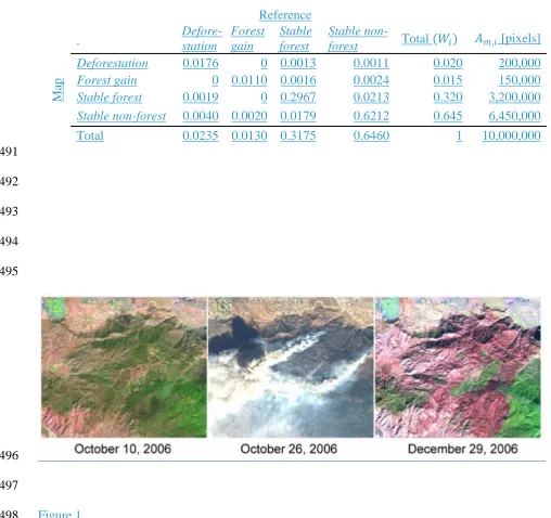
423
would be to stratify by anticipated change or predicted change, with the effectiveness of such
424
strata dependent on how well the predicted change matched with the ensuing reality of change.
425
3. Response Design
426
For the accuracy assessment objective, the response design encompasses all steps of the protocol 427
that lead to a decision regarding agreement of the reference and map classifications. For area 428
estimation, the response design provides the best available classification of change for each 429
spatial unit sampled. The Ffour major features of the response design are the spatial unit, the 430
protocol for the reference classification, and a definition of agreement. Each of these major 432
features is discussed in the following subsections. 433
3.1. Spatial Assessment Unit 434
The spatial unit that serves as the basis for the location-specific comparison of the reference 435
classification and map classification can be a pixel, polygon (or segment), or block (Stehman and 436
Wickham, 2011). The ROI is partitioned based on the chosen spatial unit (i.e., the region is 437
completely tiled by these non-overlapping spatial units). Commonly, the pixel is selected as the 438
spatial unit. The pixel is an arbitrary unit defined mainly by the properties of the sensing system 439
used to acquire the remotely sensed data or a function of the grid used to sub-divide space in a 440
raster based data set. A polygon is defined as a unit of area, perhaps irregular in shape, 441
representing a meaningful feature of land cover. For example, a polygon may be delineated from 442
a map such that the area within the polygon has the same map classification (e.g., the entire 443
polygon is stable forest or the entire polygon represents an area of change from forest to urban). 444
Polygons defined on the basis of a map will be called “map polygons.” Alternatively, a polygon 445
could be delineated on the basis of the reference classification as an area within which the 446
reference class is the same. A polygon delineated on the basis of the reference classification will 447
be called a “reference polygon”. A “block” spatial assessment unit is defined as a rectangular 448
array of pixels (e.g., a 3 x 3 block of pixels). Irrespective of the spatial unit selected, it is 449
important to note that some spatial units may be impure, that isi.e., they represent an area of 450
more than one class. Mixed pixels are, for example common, especially in coarse spatial 451
resolution data. Similarly, it is, for example, possible that a map polygon is not internally 452
homogeneous in terms of the reference classification, and a reference polygon may not be 453
algorithm would not necessarily be homogeneous in terms of either the map or the reference 455
classifications. 456
Pixels, polygons, or blocks can be used as the spatial unit in accuracy assessment. 457
Regardless of the unit chosen, a critical feature of the response design protocol is that the 458
spatially explicit character of the accuracy assessment must be retained. Practitioners should aim 459
to have reference data with an equal or finer level of detail than the data used to create the map, 460
but we make no recommendation is made regarding the choice of spatial assessment unit.
461
However, once the spatial assessment unit has been chosen, there will be good practice 462
recommendations associated with that specific unit and the choice of spatial unit also has 463
implications on the sampling design (Stehman and Wickham, 2011) and analysis. Estimates of 464
accuracy and area derived from the same map but through the use of different spatial units may 465
be unequal. 466
3.2. Sources of Reference Data 467
The reference classification can be determined from a variety of sources ranging from actual 468
ground visits to the sample locations or the use of aerial photography or satellite imagery. There
469
are two ways toTo ensure that the reference classification is of higher quality than the map 470
classification:, either the reference source has to be of higher quality than what was used to 471
create the map classification, and 2)or if using the same source material for both the map and 472
reference classifications, the process to create the reference classification has to be more accurate 473
than the process used to create the classification being evaluated.(e.g.For example, if Landsat 474
imagery is used to create the map and Landsat is the only available imagery for the accuracy 475
assessment, then the process for obtaining the reference classification has to be more accurate 476
be used to improve the quality of the reference classification, such as forest inventory data or 478
some form of vector data (e.g., roads, pipelines, or crop records). In this subsection, different 479
potential sources of reference data for assessing accuracy of change are identified and strengths 480
and weaknesses of these sources are described. 481
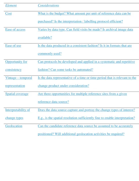
Possible reference data sources include field plots, aerial photography, forest inventory data, 482
airborne video, lidar, and satellite imagery (Table 1). Additional sources of freely accessible 483
reference data may also be opportunistically available from data mining and crowdsourcing 484
(Iwao et al., 2006; Foody and Boyd, 2013). and silvicultural records (Hyyppä et al., 2000;
485
Wulder et al., 2006a). 486
487
<< TABLE 1 HERE >> 488
489
Practical considerations regarding costs often influence the selection of reference data, or the use 490
of existing data. While existing or lower cost data may be desirable from a purchase perspective, 491
the use of disparate data sources will result in additional effort by project analysts to deal with 492
exceptions and inconsistencies. A key to using disparate data sources is to have the reference 493
data that are actually used in the accuracy assessment be, as much as possible, invariant to 494
source. For example, the creation of attributed change polygons makes the polygon the common 495
denominator, rather than the source data. Creating polygonal change units in a portable format 496
and populating a minimum set of fields to support a consistent labelling protocol is desirable. 497
The information to be recorded for each change unit is itemized in Table 2. 498
499
501
Ideally a data source is available for the entire with uniform likelihood over the ROI, 502
representing the change types and dates of interest, at a low cost. The realities versus the ideal 503
result in a series of considerations are detailed in Table 3. For instance, if the ROI is small, the 504
costs may be less of an issue and access may not be relevant. For large area projects over poorly 505
monitored areas, existing data sources are not often available so data purchase and interpretation 506
costs become the dominant criteria. The ease of interpretation and consistency of source 507
reference data permits economies in the project flow for the analysts and also promotes 508
automation of repeated activities. Further, the development of a well documented and consistent 509
change validation data set will have utility for multiple projects and purposes. 510
511
<< TABLE 3 HERE >> 512
513
Both high- and very high spatial resolution satellite data are viable candidates for reference data. 514
Imagery is typically considered as very high spatial resolution (VHSR) with a spatial resolution
515
of when pixels are sided < 1 m and high spatial resolution (HSR) with a spatial resolution of < 10 516
m. Both data sources provide information that is finer than the data used in most large area 517
monitoring projects, which would typically have use imagery with a spatial resolution of greater 518
than 10 m. At the fine spatial resolution of satellite-borne VHSR imagery, panchromatic is often 519
the only spectral information collected. The typical 400 to 900 nm panchromatic data with small 520
pixels (0.50 m in the case of WorldView-1) closely resemble large scale aerial photography and 521
can be interpreted using established aerial photograph interpretation techniques (Wulder et al., 522
DigitalGlobe® archives can be accessed through Google Earth™, with the image extents by year 524
portrayed. The presence of freely accessible high spatial resolution imagery online, freely
525
accessible, through Google Earth™ also presents low cost interpretation options. Limitations of 526
this approach include a lack of data prior to the initiation of the high spatial resolution satellite 527
commercial era (circa 2000), spatial distribution of available imagery, and the actual temporal 528
revisit of the images available. The reported temporal revisit can be on the order of days based
529
upon an ability to point the sensor head. For instance, IKONOS has off-nadir revisit of 3 to 5
530
days, with 144 days required for nadir revisit (Wulder et al. 2008b). The implication is that when
531
the sun-surface-sensor viewing geometry changes the structure captured changes, such that trees
532
evident on one image may be occluded in another. For a given on-line accessible source of 533
satellite imagery, it should not be expected that historical, archival, global coverage from launch 534
to present exist should not be expected. Regardless, the ability to view images from multiple 535
years can help determine that date when a change (e.g., a disturbance) occurred. The additional 536
context provided around particular change events aids with interpretation of change type (e.g., 537
determination of harvesting versus forest removal in support of agricultural expansion). 538
Development and sharing of a change data base, once interpreted and attributed following
539
defined procedures, leveraging Google Earth™ is a consideration for global or large area
540
accuracy assessment activities.
541
There are few, if any, reference data sources that are available with a uniform likelihood 542
globally. There are some archival datasets with wide global coverage (e.g., Kompsat); although, 543
the utility of these data sets may be limited. The utility of any given data reference data source 544
when used to capture and relate change is the date or represented by vintage of the data. While
545
less of an issue with satellite data, air photos and maps may not be of a known vintage.
Acquisition dates of historic photos are often lost, plus maps are often representative of a period,
547
not a singular date. Knowing the conditions that previously existed may not be helpful if the date 548
of change occurrence is not known. 549
Over some regions, land use change and silvicultural records may also be available to inform 550
on the land- cover change. Note that forest harvesting is a land- cover change relating a 551
successional stage, rather than a land use change (which implies a permanent change in how a 552
particular parcel of land is used – e.g., forestry to agriculture). The This distinction is important 553
for both monitoring and reporting purposes as the permanent removal of forests has differing 554
carbon consequences than a forest harvesting (Kurz, 2010). 555
While the good practice guidelines advocate for use of reference data of finer spatial 556
resolution than the map product, this is especially so for single date interpretations of the 557
reference data. Following the opening of the Landsat archive by the USGS (Woodcock et al., 558
2008), time series of imagery creates created new opportunities for using imagery of the same 559
spatial resolution (e.g., Landsat) when archival data are available. Simple visual approaches may 560
be applied, such as in Figure 1, where a change event (fire) that is evident in 2010 can be timed 561
quite precisely by the evidence captured (smoke plume) showing when the fire is occurreding. 562
This type of change dating is rather opportunistic and not to be commonly expected. 563
564
<<FIGURE 1 HERE>> 565
566
Figure 1. Landsat data can be used for the visual dating of change, with the fire event in progress 567
in Inset A, August 3, 2010, with the burned forest outcome evident in Inset B, September 20, 568
570
A more reliable means for determining the timing of change events can be from developing 571
and interrogating time series of images (Kennedy et al., 2010). To ensure the quality of time 572
series transitions developed, Cohen et al. (2010) created a logic and tool for determining the 573
timing and nature of changes captured (TimeSync, http://timesync.forestry.oregonstate.edu/). 574
Based upon the image collection and archiving protocols present through the history of Landsat, 575
the spatial and temporal coverage of imagery is not uniform. The temporal precision possible for 576
dating changes based upon time series analysis is likely weaker for locations that already have a 577
paucity of data. This situation is due to the historic practices followed at given Landsat receiving 578
stations through to the commercial era (during the 1980s) when fewer images were collected and 579
archived (Wulder et al., 2012). It should not be assumed that the temporal density possible for 580
the conterminous United States is possible for all other regions (Schroeder et al., 2011). 581
Another critical aspect of the response design is that the change period represented by the 582
reference classification must be synchronous with the change period of the classification. 583
Consider a map representing change between 2000 and 2010. To capture near anniversary dates
584
(within year) and athe northern hemisphere peak photosynthetic period, the imagery used for this 585
hypothetical project was collected July 15, 2000, and 10 years later, July 15 2010. The reference 586
data should be collected in 2010, but ideally not after July 15 (assuming similar satellite overpass 587
times) to avoid confusion. Data collected after July 15, 2010 will have to be vetted to ensure the 588
change present in the reference data did not occur after the product date of the change map. 589
Imagery from the same year is desired but may not always be possible. As such, it is required 590
that the change reference data includes approximates the date the change occurred as precisely as 591
change periods between the map and reference classifications would be a major source of 593
reference data error. 594
3.3. Reference Labelling Protocol 595
The labelling protocol refers to the steps in the response design that take the information 596
provided by the reference data and convert that information to the label or labels constituting the 597
reference classification. Labelling is far from trivial with numerous definitions for land- cover 598
classes in use (cf. Comber et al., 2008 ) although recent developments such as the FAO’s Land 599
Cover Classification system (LCCS) may act to enhance interoperability (Ahlqvist, 2008). The 600
labelling protocol should also include specification of a minimum mapping unit (MMU) for the 601
reference classification. The MMU can have important implications for accuracy assessment and 602
area estimation. For example, increasing the size of the MMU will lead to a reduction in the 603
representation of classes that occupy small, often fragmented, patches (Saura, 2002). Changing 604
the MMU can also impact on accuracy estimates, although the effect is most apparent when a 605
large change is made (Knight and Lunetta, 2003). Clearly, sSmall patches present a challenge to 606
mapping (cf. He et al., 2011) and the accuracy of their mapping will degrade as the MMU is 607
increased. However, but it is possible that overall map accuracy may increase with a larger
608
MMU, making it is important to ensure that attention is focused on an appropriate measure of 609
accuracy for the application in-hand. The precise effects of the MMU will vary as a function of 610
the land- cover mosaic under study and the imagery used. The MMU specified for the response 611
design does not necessarily have to match the MMU specified for the map. In fact, if the 612
reference classification is intended to apply to a variety of maps, it would be likely that the 613
MMU of the reference classification does not match the map classification for all maps that 614
patches or features than can be distinguished from the map so a smaller MMU will be possible 616
for the reference classification. 617
The easiest case for the labelling protocol occurs when the assessment unit is homogeneous 618
and a single reference class label can be assigned (the reference class could be a type of change). 619
But oOften, however, the situation will be more complex making class labelling less certain. For 620
example, the assessment unit may contain a mixture of classes, and even if the unit is 621
homogeneous, it may be difficult to assign a single label (e.g., change type) because the unit is 622
not unambiguously one of the classes in the legend but instead falls between two of the discrete 623
class options in the legend (i.e., land- cover classes are a continuum represented on a discrete 624
scale). A variety of options exist for labelling a unit when a single reference label does not 625
adequately represent the uncertainty of a unit. One or more alternate reference class labels can be 626
assigned to account for ambiguity in the reference classification. Another option when defining 627
agreement is to construct a weighted agreement based on how closely the different classes are 628
related. For example, in the GlobCover assessment, a “matrix” of class relationships was 629
established (Mayaux et al., 2006, GLC2000). A fuzzy reference labelling protocol may also be 630
employed, for examplesuch as the linguistic scale devised by Gopal and Woodcock (1994) or a 631
fuzzy membership vector in which the reference label for a unit specifies a membership value for 632
each class (Foody, 1996; Binaghi et al., 1999). Another option for mixed units is to specify the 633
proportion of area of each class present in the unit (Foody et al., 1992; Lewis and Brown, 2001). 634
A different characterization of uncertainty in the reference classification is obtained by assigning 635
a confidence rating that represents the interpreter’s perception of uncertainty in the reference 636
classification for that unit. For example, low, moderate and high confidence ratings would 637
correct. Typically this information can then be used in the analysis to subset results by 639
confidence rating (Powell et al., 2004; Wickham et al., 2001, Table 4). 640
The response design should include protocols to enhance consistency of the reference class 641
labelling. For example, interpretation keys should be created if visual assessment is used to 642
obtain the reference classification (Kelly et al., 1999) and specific instructions to translate 643
quantitative field data into reference labels should be provided and documented. If multiple 644
interpreters are used, training interpreters to ensure consistency is critical. Interpreters should be 645
in communication throughout the process to discuss and review difficult cases and to agree upon 646
a common approach to labelling such cases. Difficult cases should be noted for future reference 647
and consensus development (e.g., the imagery is retained and accessible, and the decision 648
process leading to the reference label of the case is documented). Rather than solely visual 649
approaches, entire high spatial resolution images can be classified, with the underlying imagery 650
also maintained and accessible as support information to the accuracy assessment (that is, to 651
gain/ensure confidence in the categories selected for a given location). 652
3.4. Defining Agreement 653
Once the map and reference classifications have been obtained for a given spatial unit, rules for 654
defining agreement must be specified before proceeding to the analyses that quantify accuracy. 655
In the simplest case, a single class label is present for the map and a single label is provided by 656
the reference classification. If these labels agree, the map class is correct for that unit, ;and if the 657
labels disagree, the type of misclassification is readily identified. Defining agreement becomes 658
more complex if the assessment unit is not homogeneous or if more than a single one class label 659
is assigned by the map or reference classification. For example, if the reference classification 660
the map label and either the primary or secondary reference label. If the reference classification 662
consists of a vector of proportions of area of the classes present in the assessment unit (e.g., the 663
area proportions of the classes are 0.2, 0.5, and 0.3), agreement can be defined as the proportion 664
of area for which the map and reference labels are the same. The critical feature of the protocol 665
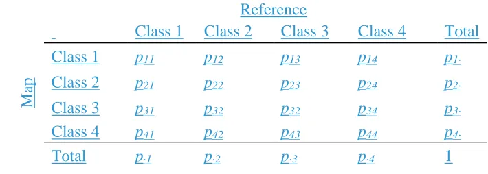
for defining agreement is that it allows construction of an error matrix in which the elements of 666
the matrix represent proportion of area of agreement and disagreement between the map and 667
reference classifications. These proportions (in terms of area) achieve the necessary spatially 668
explicit assessment of map accuracy and the requirements for area estimation. 669
3.5. Reference Classification Uncertainty: Geolocation and Interpreter Variability 670
In an ideal case, the reference classification is based on a reference data set of such quality that 671
the sample labels represent the ground truth (i.e. a “gold standard” reference data set). However, 672
the reference classification is subject to uncertainty, and an assessment of this uncertainty should 673
be conducted. Small errors in the reference data set can lead to large biases of the estimators of 674
both classification accuracy and class area (Foody, 2010; 2013). Two potential sources of 675
uncertainty in the reference classification are the uncertainty associated with spatial co-676
registration of the map and reference location (Pontius, 2000) and uncertainty associated with the 677
interpretation of the reference data (Pontius and Lippitt, 2006). 678
Geolocation error is defined as a mismatch between the location of the spatial assessment 679
unit identified from the map and the location identified from the reference data. The response 680
design should be constructed to minimize geolocation error. For instance, it is common for plots 681
to have a GPS position. The quality of the GPS position can be related by to the type of 682
instrument used, which can provide an indication of spatial precision. The length of time, 683
that can be recorded. The magnitude of geolocation error should be characterized by 685
documenting the spatial location quality of the map and reference data sources (e.g., GPS units, 686
aerial photography, or satellite imagery). If airborne imagery is to be used, aircraft positioning 687
and pointing information should be collected. The GPS location of the aircraft does not 688
necessarily indicate the position of the point on the ground that is captured in photographic or 689
video data. A slight roll of the aircraft can create a mismatch between the recorded and actual 690
positions. Error in the classification may be incorrectly indicated due to these spatial 691
mismatches, especially for smaller change events or rare classes. 692
Interpreter uncertainty can be separated into two parts: 1) interpreter bias is defined as an 693
error in the assignment of the reference class to the spatial unit; 2) interpreter variability is a 694
difference between the reference class assigned to the same spatial unit by different interpreters 695
(i.e., interpreter variability is the complement of among interpreter agreement). Although iIdeally 696
an assessment of both interpreter bias and interpreter variability would be conducted, ; in 697
practice, assessing only interpreter variability may be feasible. The difficulty hindering 698
assessment of interpreter bias is whether a “gold standard” of truth exists against which the 699
interpreted reference classification can be compared. For example, on-the-ground reference data 700
may serve to establish the gold standard of truth for land cover at a single date, but a gold 701
standard for change based on field visits would be much more difficult and costly to establish. 702
Comparison of interpreters to an “expert” interpreter is a practical but less satisfying option for 703
quantifying interpreter bias and the success of this approach depends on how closely the expert 704
classification mimics the gold standard. A distinction between the accuracy assessment of land 705
cover and change does exist, whereby the continuous nature of land cover benefits more from 706
informative. For example, slower continuous changes may benefit from field visits, but rapid 708
stand replacing disturbances may not. The date of change, if not captured in silvicultural records 709
or fire maps, may actually be better captured from imagery of known vintage than through field 710
visits (Cohen et al., 2010). 711
If multiple interpreters or interpreter teams are providing the reference classification,
712
interpreter variability can be assessed by having interpreters classify a common sample of
713
locations. Ideally, the sample would include locations covering a variety of classes to allow
714
evaluating how interpreter variability differs by class (e.g., do interpreters consistently agree for
715
some classes, but not others). The quality of the interpreters in terms of the accuracy of their
716
labelling may also be assessed directly from the data generated (Foody et al., 2013). If this
717
evaluation sample is selected using a probability sampling design (see Section 2), estimates of
718
interpreter variability will have a strong inferential basis and results from the sample can be
719
rigorously inferred to the population of all interpretations. If multiple interpreters operating
720
independently are employed to determine the reference classification for each sample location, a
721
number of considerations may affect the decision of how many interpreters are used. Wulder et
722
al. (2007) who used seven interpreters in a land cover labelling protocol, detail the issues that
723
arise when using multiple interpreters, noting common disagreement between interpreters,
724
especially for more refined and rare classes. Ensuring that consensus is reached, rather than an
725
aggregation of independent interpretations, is also possible. Also using airborne video data,
726
Powell et al. (2004) required five interpreters to agree upon a specific class, with the outcome
727
then treated as a “gold standard”. While some disagreement could be linked to difficulty in
728
identifying the vegetation in the video, other sources of disagreement included data entry error
729
and misreading of sample labels. These are sources of error that can be mitigated by using