Robust and efficient parametric face alignment

Robust and Efficient Parametric Face Alignment

Georgios Tzimiropoulos

Stefanos Zafeiriou

_{Dept. of Computing,}

Imperial College London

180 Queen’s Gate

London SW7 2AZ, U.K.

{gt204,s.zafeiriou,m.pantic}@imperial.ac.uk

Maja Pantic

∗

_EEMCS

University of Twente

Drienerlolaan 5

7522 NB Enschede

The Netherlands

Abstract

We propose a correlation-based approach to parametric object alignment particularly suitable for face analysis ap-plications which require efficiency and robustness against occlusions and illumination changes. Our algorithm regis-ters two images by iteratively maximizing their correlation coefficient using gradient ascent. We compute this corre-lation coefficient from complex gradients which capture the orientation of image structures rather than pixel intensities. The maximization of this gradient correlation coefficient re-sults in an algorithm which is as computationally efficient asℓ2norm-based algorithms, can be extended within the in-verse compositional framework (without the need for Hes-sian re-computation) and is robust to outliers. To the best of our knowledge, no other algorithm has been proposed so far having all three features. We show the robustness of our algorithm for the problem of face alignment in the presence of occlusions and non-uniform illumination changes. The code that reproduces the results of our paper can be found at http://ibug.doc.ic.ac.uk/resources.

1. Introduction

Object alignment methods aim at finding the transforma-tion or deformatransforma-tion which minimizes the discrepancies be-tween two or more images/objects. In automated face anal-ysis, these discrepancies usually stem from rigid head mo-tions induced by observing faces at different time instances and from different viewpoints as well as from non-rigid fa-cial deformations induced by fafa-cial expressions. Alignment methods aim at estimating these motions and, therefore, play a central role in the efficacy and robustness of high-level applications such as face recognition, speech reading

∗_{This work has been funded by the European Research Council under}

the ERC Starting Grant agreement no. ERC- 2007-StG-203143 (MAH-NOB).

and facial expression analysis.

In this work, we focus on object alignment methods based on gradient descent optimization. Since the first al-gorithm of this type, the Lucas-Kanade (LK) alal-gorithm [1], gradient descent has become one of the key ingredients in face alignment algorithms. Numerous extensions to the LK algorithm have been proposed to address issues related to efficiency [2–5], generalization capacity [2, 6, 7], opti-mization [8, 9] and robustness [10–13]. Most prior work is based on ℓ2 norm minimization. The ℓ2 norm is the

standard choice [1, 2, 5, 13, 14], as it can result in compu-tationally efficient algorithms. Perhaps, the most notable example of such algorithms is the inverse compositional al-gorithm proposed by Baker and Matthews [4, 5]. At each iteration, the method solves a linear least squares problem with the Hessian pre-computed and constant across itera-tions. As usual, the choice of the norm imposes a trade-off between robustness and computational complexity. Robust approaches typically replace theℓ2norm with a robust error

function [10, 11]. Such methods solve a re-weighted least squares problem, where the weights are updated at each iteration. This additional computation makes them much slower. For example, replacing theℓ2 norm with a robust

function within the inverse compositional framework, re-quires the re-computation of the Hessian at each iteration, resulting in a less efficient algorithm [11].

of mild assumptions, is canceled out by applying the cosine kernel. Thus, image regions corrupted by outliers result in approximately zero correlation and therefore do not bias the estimation of the transformation parameters significantly.

To maximize the gradient correlation coefficient, we for-mulate and solve a continuous optimization problem. The proposed methodology results in a computationally efficient and robust alignment algorithm. In particular, our algo-rithm is as efficient asℓ2norm-based algorithms, can be

ex-tended within the inverse compositional framework (with-out the need for Hessian re-computation) and is robust to outliers caused by occlusions and non-uniform illumination changes. To the best of our knowledge, no other algorithm has been previously proposed having all three features.

To evaluate the performance of our scheme, we consid-ered the problem of face alignment in the presence of oc-clusions and non-uniform illumination changes using hun-dreds of real face pairs taken from the AR [19] and Yale B [20] databases. Our results show that, unlike previously proposed schemes, our algorithm can cope with such cum-bersome problems.

Summarizing our contributions, in this paper

• We propose the maximization of the correlation of im-age gradient orientations as a new cost function for ro-bust gradient ascent face alignment.

• We formulate and solve the continuous optimization problems which result in the forward additive and in-verse compositional versions of our algorithm.

• We present results for very challenging alignment cases which have not been previously examined. Ta-ble 1 presents a comparison between our experiments and the ones reported in related alignment papers. The code that reproduces the results of our paper can be found at http://ibug.doc.ic.ac.uk/resources.

2. Gradient-based correlation coefficient

Assume that we are given the image-based representa-tions of two objectsIi ∈ ℜm1×m2,i= 1,2. We define the

complex representation which combines the magnitude and the orientation of image gradients asGi =Gi,x+jGi,y,

wherej =p

(−1),Gi,x =Fx⋆Ii,Gi,y =Fy⋆Iiand Fx,Fy are filters used to approximate the ideal

differenti-ation operator along the image horizontal and vertical di-rection respectively. We also denote byP the set of indices corresponding to the image support and bygi=gi,x+jgi,y

theN−dimensional vectors obtained by writingGiin

lex-icographic ordering, whereN is the cardinality ofP. The gradient correlation coefficient is defined as

s,ℜ{gH₁ g2}, (1)

whereℜ{.}denotes the real part of a complex number and H denotes the conjugate transpose [15]. Using ri(k) ,

q

g2

i,x(k) +g2i,y(k)andφi(k),arctan

gi,y(k)

gi,x(k), we have

s,X

k∈P

r1(k)r2(k) cos[∆φ(k)], (2)

where∆φ,φ₁−φ₂.

The magnitudesr_iin (2) suppress the contribution of ar-eas of constant intensity level which do not provide useful features for object alignment. Note, however, that the use of gradient magnitude does not necessarily result in robust al-gorithms. For example, the authors in [21] have shown that the gradient magnitude varies drastically with the change in the direction of the light source.

The key to the robustness of the proposed scheme is the correlation of gradient orientations which takes the form of the sum of cosines of gradient orientation differences [15, 17]. To show this [15, 18], assume that there ex-ists a subset Po ⊂ P corresponding to the set of pixels

corrupted by outliers. By using the normalized gradients

˜

gi = ˜gi,x+jg˜i,y, where ˜gi,x(k) = gi,x(k)/|gi(k)|and

˜

g_i,y(k) =g_i,y(k)/|g_i(k)|, so thatr_i(k) = 1∀k, the value of this gradient correlation coefficient inPois

qo,

X

k∈Po

cos[∆φ(k)]. (3)

To compute the value of qo, we note that in Po the

im-ages arevisually dissimilar/unrelated, so that locally do not match. It is therefore not unreasonable to assume that for any spatial locationk, the difference in gradient orientation

∆φ(k)can take any value in the range[0,2π)with equal probability. Thus, we can assume that∆φis a realization of a stationary random processu(t)which∀tfollows a uni-form distributionU(0,2π). Given this, it is not difficult to show that, under some rather mild assumptions, it holds

qo=

X

k∈Po

cos[∆φ(k)]≃0. (4)

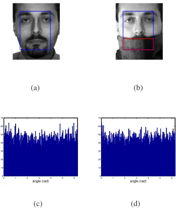
This assumption has been shown to be valid using the Kolmogorov-Smirnoff test for more than 70.000 pairs of vi-sually unrelated imagesin [18]. As an example, in Fig. 1 (a)-(b), we assume that the scarf is visually unrelated to the face. Po here corresponds to the part of the face occluded

by the scarf defined by the red rectangle. Fig. 1 (c) plots the distribution of∆φinPo, while Fig. 1 (d) shows the

histogram of uniformly distributed samples obtained with Matlab’s rand function. As in [18], to verify that∆φis uni-formly distributed, we used the Kolmogorov-Smirnov test [22] to test the null hypothesisH0 : ∀k ∈ Po, ∆φ(k) ∼

the samples obtained with Matlab’srandfunction, the null hypothesis was accepted withp= 0.48.

Overall, unlike standard correlation (i.e. the inner prod-uct) of pixel intensities where the contribution of outliers can be arbitrarily large, the effect of outliers is approxi-mately canceled out inPo. Corrupted regions result in

ap-proximately zero correlation and thus do not bias the esti-mation of the transforesti-mation parameters.

(a) (b)

0 1 2 3 4 5 6 0

10 20 30 40 50 60 70

angle (rad)

(c)

0 1 2 3 4 5 6 0

10 20 30 40 50 60 70

angle (rad)

(d)

Figure 1. (a)-(b) A pair of faces from the AR database. The re-gion of interest is defined by the blue rectangle. The corrupted regionPois defined by the red rectangle. (c) The distribution of

∆φinPo. (d) The distribution of samples (uniformly distributed)

obtained with Matlab’s rand function.

3. Gradient Orientation in Face Analysis

The use of gradient orientation as useful features for face analysis is by no means proposed for the first time in this work. Examples of previous work can be found in [21, 23, 24]. However, most prior work proposes gradient orientations as features for achieving insensitivity in non-uniform illumination variations. On the contrary, what is highlighted in [15, 18] as well as in this work is why gradi-ent origradi-entations can be used for outlier-robust (for example occlusion-robust) face analysis.

Regarding face alignment, perhaps what is somewhat related to the proposed scheme is the Active Appearance Model proposed in [24]. We underline two important differ-ences between our algorithm and the method of [24]. First, as [24]doesemploy the gradient magnitude (even for nor-malization) for feature extraction, it is inevitably less robust to outliers. Second, no attempt to exploit the relation be-tween image gradients and pixel intensities is made. More specifically, the gradient-based features in [24] are treated

just as pixel intensities which are then used for regression-basedobject alignment. On the contrary, we make full use of the relation between image gradients and pixel intensities to formulate and solve acontinuous optimizationproblem. This results in a dramatic performance improvement as Sec-tion 5 illustrates.

4. Robust and efficient object alignment

Parametric object alignment methods assume thatI1and

I2are related by a parametric transformation, i.e.

I1(xk) =I2(W(xk;p)),∀k∈ P, (5)

whereW(xk;p)is the parametric transformation with

re-spect to the image coordinatesxk = [x1(k),x2(k)]T and p = [p(1), . . . ,p(n)]T _{is the vector of the unknown}

pa-rameters. Next,pis estimated by minimizing an objective function which is typically the ℓ2 norm of the difference

E=I1−I2. The minimization is performed in an iterative

fashion after making a first or second order Taylor approxi-mation to eitherI1orI2.

4.1. The quantity maximized

In this section, we propose the maximization of the cor-relation of image gradient orientations as a new cost func-tion for robust gradient descent face alignment. In particu-lar, to estimatep, we wish to maximize

q=X

k∈P

cos[∆φ(k)]. (6)

By using the normalized gradients ˜gi, simple calculations

show that (6) is equivalent to

q=X

k∈P

˜

g1,x(k)˜g2,x(k) + ˜g1,y(k)˜g2,y(k). (7)

Note, however, that a first order Taylor expansion of g˜1

or ˜g2 with respect to ∆p yields a linear function of ∆p

which is maximized as∆p → ∞. To alleviate this prob-lem without resorting to the second order Taylor expansion as in [25], we follow an approach similar to [14]. To pro-ceed, we note that as||g˜2(k)||2= 1,∀k∈ P, the proposed

cost function is exactly equal to

q=

P

k∈P˜g1,x(k)˜g2,x(k) + ˜g1,y(k)˜g2,y(k)

q P

k∈Pg˜22,x(k) + ˜g22,y(k)

, (8)

but if we linearize˜g2in the above expression, the

denomi-nator will not be equal to 1 andqwill become a non-linear function of ∆p. Finally, using vector notation, our cost function becomes

q= g˜

T

1,x˜g2,x+ ˜gT1,y˜g2,y

q

˜

gT

2,xg˜2,x+ ˜g2T,yg˜2,y

To maximizeqwith respect top, we first make the de-pendence ofg˜2(k)onpexplicit by writing˜g2[p](k). Then, we maximize iteratively by assuming that the current esti-mate ofpis known and by looking for an increment ∆p

which maximizes our objective function in (9) with respect to∆p.

4.2. The forward-additive gradient correlation

al-gorithm

In this section, we describe how to maximize the pro-posed cost function in (9) using the forward-additive max-imization procedure. In this framework [1, 5], at each iter-ation, we maximize (9) with respect to∆pwhereg2 ←−

g2[p+ ∆p]. Once we obtain∆p, we update the param-eter vector in an additive fashionp ←− p+ ∆pand use this new value of p to obtain the updated warped image

I2(W(x;p)).

We start by noting thatg2[p](k)is the complex gradient ofI2(W(x;p))with respect to the original coordinate sys-tem evaluated atx = x_k. This gradient is different from the gradient ofI2 calculated at the first iteration and then

evaluated atW(x_k;p), which, for convenience, we will de-note byh2[p](k). That is, h2[p] =h2,x[p] +jh2,y[p]is

obtained by writingG2,x(W(x;p)) +jG2,y(W(x;p))in

lexicographic ordering, whereG2 =G2,x+jG2,yis

as-sumed to be computed at the first iteration. In a similar fash-ion, we denote byh2,xx[p],h2,yy[p]andh2,xy[p], the

vec-tors obtained by writing in lexicographic ordering the sec-ond partial derivatives ofI2,G2,xx,G2,yyandG2,xy,

com-puted at the first iteration and, then, evaluated atW(x;p). Let us also write W(x;p) = [w1(x;p),w2(x;p)]T_{, so}

that the matrix derivative with respect to a vector a = [a(1), . . . ,a(m)]T _{is given by}

∂W

∂a =

" _∂w

1

∂a(1) . . .

∂w₁

∂a(m)

∂w₂

∂a(1) . . .

∂w₂

∂a(m)

#

. (10)

By definition we have

g2[p](k) , [g2,x[p](k) g2,y[p](k)]

, ∂I2(W_∂x(x;p))

_x

=xk

= ∇WI2[p](k) ∂W

∂x

_x

=xk

, (11)

where∇WI2[p](k),[h2,x[p](k) h2,y[p](k)]. By

apply-ing the chain rule and noticapply-ing that∇W∂_∂W_x = 0, we also have

" _∂g₂,x[p](k)

∂p

∂g2,y[p](k)

∂p

#

= ∂W

∂x

x=xk

!T

×

h2,xx[p](k) h2,xy[p](k) h2,yx[p](k) h2,yy[p](k)

_∂W

∂p.

(12)

We assume that the current estimate of p is known. The key point to make derivations tractable is to recall that

˜

g2,x[p](k)≡cosφ2[p](k)and˜g2,y[p](k)≡sinφ2[p](k)

where

φ₂[p](k) = arctang2,y[p](k)

g2,x[p](k)

. (13)

By performing a first order Taylor expansion on ˜g2,x[p+

∆p](k), we get

˜

g2,x[p+ ∆p](k)≈cosφ2[p](k) +

∂cosφ₂[p](k)

∂p ∆p.

(14) By repeatedly applying the chain rule, we get

∂cosφ₂[p](k)

∂p =−sinφ2[p](k)j[p](k), (15)

wherej[p](k)is a1×nvector given by

j[p](k) = cosφ2[p](k)

∂g2,y[p](k)

∂p −sinφ2[p](k)

∂g2,x[p](k)

∂p

q

g₂2_,x[p](k) +g2_2,y[p](k)

.

(16) Using vector notation, we can write

˜

g2,x[p+ ∆p]≈cosφ2[p]−Sφ[p]⊙J[p]∆p, (17)

where S_φ[p]is the N ×nmatrix whosek−th row hasn elements all equal tosinφ₂[p](k),J[p]is theN×n Jaco-bian matrix whosek−th row hasnelements corresponding toj[p](k)and⊙denotes the Hadamard product. Very sim-ilarly, we can derive

˜

g2,y[p+ ∆p]≈sinφ2[p] +Cφ[p]⊙J[p]∆p, (18)

where Cφ[p]is theN×nmatrix whosek−th row hasn

elements all equal tocosφ₂[p](k).

Let us denote byS∆φ[p]theN×1vector whosek−th

element is equal tosin(φ₁(k)−φ₂[p](k)). Then, by plug-ging (17) and (18) into (9), and after some calculations, our cost function becomes

q(∆p) = qp+S

T

∆φJ∆p

p

N+ ∆pT_JT_J∆p, (19)

whereqp= cosφT1 cosφ2+sinφT1 sinφ2is the correlation

of gradient orientations betweenI1 andI2(W(x;p)), and

we have dropped the dependence of the quantities onpfor notational simplicity. Finally, the maximization of (19) with respect to ∆pcan be obtained by applying the results of [14]. In particular, the maximum value is attained for

∆p=λ(JTJ)−1_JT_S

∆φ, (20)

4.3. The inverse-compositional gradient correlation

algorithm

In this section, we show how to maximize the proposed cost function in (9) using the inverse-compositional maxi-mization procedure. In this framework [4, 5], a change of variables is made to switch the roles of I1 andI2 and the

updated warp is obtained in a compositional (rather than additive) fashion. Thus, our cost function becomes

q= (˜g2,x[p])

T_(˜g

1,x[∆p]) + (˜g2,y[p])T(˜g1,y[∆p])

p

(˜g1,x[∆p])T(˜g1,x[∆p]) + (˜g1,y[∆p])T(˜g1,y[∆p])

(21) with respect to∆pand, at each iteration,I2is updated using

W(x;p)←−W(x;p)◦(W(x; ∆p))−1_{, where◦denotes}

composition.

Similarly to [5], we assume thatW(x;0) = x. This, in turn, impliesg1[∆p]≡h1[∆p]which greatly simplifies the derivations. As before, we perform a Taylor approxima-tion to˜g1,x[p], but this time around zero. This gives

˜

g1,x[∆p]≈cosφ1[0]−Sφ[0]⊙J[0]∆p, (22)

whereSφ[0]is theN×nmatrix whosek−th row hasn

el-ements all equal tosinφ₁[0](k)andJ[0]is theN×n Jaco-bian matrix whosek−th row hasnelements corresponding to the1×nvector

j[0](k) = cosφ1[0](k)

∂g1,y[0](k)

∂p −sinφ1[0](k)

∂g1,x[0](k)

∂p

q

g₁2_,x[0](k) +g2_1,y[0](k)

(23) and

" _∂g₁,x[0](k)

∂p

∂g₁,y[0](k)

∂p

#

=

g1,xx[0](k) g1,xy[0](k) g1,yx[0](k) g1,yy[0](k)

∂W

∂p

_p=0

.

Similarly, forg˜1,y[∆p], we get

˜

g1,y[∆p]≈sinφ1[0] +Cφ[0]⊙J[0]∆p, (24)

whereCφ[0]is theN×nmatrix whosek−th row hasn

ele-ments all equal tocosφ₁[0](k). Notice that all terms in (22) and (24) do not depend onpand, thus, are pre-computed and constant across iterations.

Let us denote byS∆φ[p]theN×1vector whosek−th

element is equal tosin(φ₂[p](k)−φ₁(k)). Then, by drop-ping the dependence of the above quantities on pand0, our objective function will be again given by (19) while the optimum∆pwill be given by (20).

4.4. Computational complexity

A simple inspection of our algorithms shows that the most computationally expensive step is the calculation of

JT_{Jin (19) which requiresO(n}2_{N)operations. The cost}

of all other steps is at mostO(nN)(sinceN ≫n). In the inverse compositional maximization procedure, JTJ and its inverse is pre-computed and, therefore, the complexity per iteration isO(nN). Finally, an un-optimized MATLAB version of our algorithm takes about 0.03-0.04 seconds per iteration while the original inverse compositional algorithm takes about 0.02-0.03 seconds per iteration. We note that an optimized version of the original inverse compositional algorithm, as the core part of Active Appearance Model fit-ting, has been shown to track faces faster than 200 fps [7].

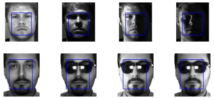
Figure 2. Examples of images used in our experiments (prior to the application of an affine transformation). The blue rectangle defines the region of interest.

5. Face alignment experiments

We assessed the performance of our algorithms, which we coin GradientCorr-FA and GradientCorr-IC, using the performance evaluation framework proposed in [5] which has now become the standard evaluation procedure [9, 12– 14]. We present results and comparison with previous work for very challenging alignment cases which have not been previously examined. Table 1 presents a comparison be-tween our experiments and the ones reported in object align-ment papers which also adopt the evaluation framework of [5]. In addition to the standard “Takeo” experiment, we considered, for the first time (to the best of our knowledge), the problem of face alignment in the presence of real oc-clusions and non-uniform illumination changes using hun-dreds of real faces taken from the AR [19] and Yale B [20] databases.

con-Methods Number of Real image Transformation Illumination Occlusion AWGN Compared

image pairs pair Affine/ with

considered Homography

[5] 4 (Takeo+3) No Yes/Yes No No Yes [5] [11] 6 (Takeo) No Yes/No No Yes (synthetic) No [5, 11] [12] 3 Yes Yes/No Yes (natural) No No [5] [14] 1 (Takeo) No Yes/No Yes (synthetic) No Yes [5, 6] [13] NA (Multi-Pie [26]) Yes Yes/No Yes (natural) No No [5]

[9] 11 No Yes/No Yes (synthetic) No Yes [5] Proposed 182 (Takeo + Yale +AR) Yes Yes/No Yes (natural) Yes (real) Yes [5, 11, 13, 14]

Table 1. Comparison between the experimental settings reported in object alignment papers following the evaluation framework of [5].

1 2 3 4 5 6 7 8 9 10

0 0.1 0.2 0.3 0.4 0.5 0.6 0.7 0.8 0.9 1

Frequency of Convergence

Point Standard Deviation Takeo: No Smoothing, No Noise

LK−fa LK−ic GradientCorr−fa GradientCorr−ic

(a)

1 2 3 4 5 6 7 8 9 10

0 0.1 0.2 0.3 0.4 0.5 0.6 0.7 0.8 0.9 1

Frequency of Convergence

Point Standard Deviation Takeo: Smoothing, No Noise

LK−fa LK−ic GradientCorr−fa GradientCorr−ic

(b)

1 2 3 4 5 6 7 8 9 10

0 0.1 0.2 0.3 0.4 0.5 0.6 0.7 0.8 0.9 1

Frequency of Convergence

Point Standard Deviation Takeo: Smoothing, Noise

LK−fa LK−ic GradientCorr−fa GradientCorr−ic

(c)

Figure 3. Frequency of Convergence vs Point Standard Deviation for Takeo image [5]. (a) No Smoothing, No Noise (b) Smoothing, No Noise (c) Smoothing, Noise. LK-fa: black-x. LK-IC: black-♦. GradientCorr-fa: blue-◦. GradientCorr-IC: blue-.

1 2 3 4 5 6 7 8 9 10

0 0.1 0.2 0.3 0.4 0.5 0.6 0.7 0.8 0.9 1

Frequency of Convergence

Point Standard Deviation Yale: No Smoothing

LK−ic ECC−ic IRLS−ic GaborFourier−ic GradientImages−ic GradientCorr−ic

(a)

1 2 3 4 5 6 7 8 9 10

0 0.1 0.2 0.3 0.4 0.5 0.6 0.7 0.8 0.9 1

Frequency of Convergence

Point Standard Deviation AR: No Smoothing (Occlusion)

LK−ic ECC−ic IRLS−ic GaborFourier−ic GradientImages−ic GradientCorr−ic

(b)

1 2 3 4 5 6 7 8 9 10

0 0.1 0.2 0.3 0.4 0.5 0.6 0.7 0.8 0.9 1

Frequency of Convergence

Point Standard Deviation AR: No Smoothing (Occlusion+illumination)

LK−ic ECC−ic IRLS−ic GaborFourier−ic GradientImages−ic GradientCorr−ic

(c)

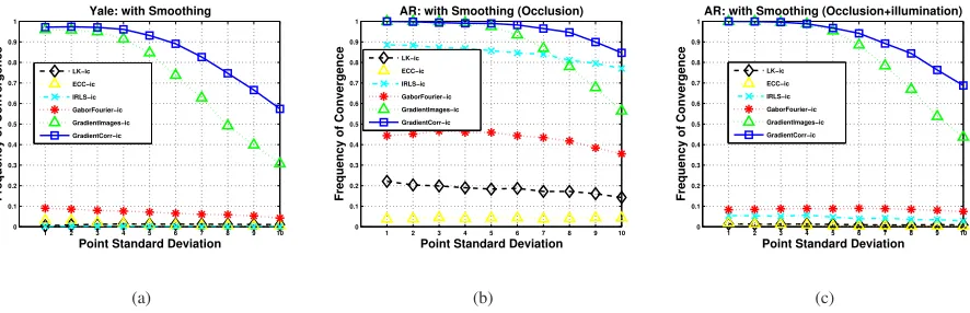
Figure 4. Average Frequency of Convergence vs Point Standard Deviation for Yale and AR databases. No smoothing was used. (a) Yale (b) AR-Occlusion (c) AR-Occlusion+illumination. LK-IC: black-♦. ECC-IC: yellow-△. IRLS-IC: cyan-x. GaborFourier-IC: red-*. GradientImages-IC: green-△. GradientCorr-IC: blue-.

sidered to have converged if the final RMS point error was less than n1 pixels after 30 iterations. We obtained these

averages using, for eachσ,n2randomly generated warps.

5.1. Experiments using the Takeo image

We started by reproducing to some extend the exper-imental setting of [5] using the Takeo image. We used n1 = 1pixel and, for eachσ,n2 = 1000randomly

gener-ated warps. We assessed the performance of the forward ad-ditive and inverse compositional versions of our algorithm

and the LK algorithm. We considered 3 cases. The first case was with no Gaussian smoothing prior to the calcula-tion of image derivatives and no AWGN (Additive White Gaussian Noise). The second case was with smoothing but no AWGN. Finally, the third case was with both smooth-ing and AWGN of variance equal to 10 added to both the template and the target image. Fig. 3 shows the obtained average frequency of convergence.

un-1 2 3 4 5 6 7 8 9 10 0

0.1 0.2 0.3 0.4 0.5 0.6 0.7 0.8 0.9 1

Frequency of Convergence

Point Standard Deviation Yale: with Smoothing

LK−ic ECC−ic IRLS−ic GaborFourier−ic GradientImages−ic GradientCorr−ic

(a)

1 2 3 4 5 6 7 8 9 10

0 0.1 0.2 0.3 0.4 0.5 0.6 0.7 0.8 0.9 1

Frequency of Convergence

Point Standard Deviation AR: with Smoothing (Occlusion)

LK−ic ECC−ic IRLS−ic GaborFourier−ic GradientImages−ic GradientCorr−ic

(b)

1 2 3 4 5 6 7 8 9 10

0 0.1 0.2 0.3 0.4 0.5 0.6 0.7 0.8 0.9 1

Frequency of Convergence

Point Standard Deviation AR: with Smoothing (Occlusion+illumination)

LK−ic ECC−ic IRLS−ic GaborFourier−ic GradientImages−ic GradientCorr−ic

(c)

Figure 5. Average Frequency of Convergence vs Point Standard Deviation for Yale and AR databases. Smoothing was used. (a) Yale (b) AR-Occlusion (c) AR-Occlusion+illumination. LK-IC: black-♦. ECC-IC: yellow-△. IRLS-IC: cyan-x. GaborFourier-IC: red-*. GradientImages-IC: green-△. GradientCorr-IC: blue-.

reasonable, as the affine distorted image was generated di-rectly from the original image. In this case, there are no outliers, and as our algorithms remove some amount of in-formation (most importantly the gradient magnitude), they inevitably perform worse. As Fig. 3 (b) illustrates, Gaus-sian smoothing improves the performance of all methods by providing a larger region of attraction. The performance gap between the LK and the proposed methods is now sig-nificantly smaller. Finally, as Fig. 3 (c) shows, if smoothing is used, none of the methods is affected too much by the AWGN even for a large noise variance (In fact, the perfor-mance of the LK methods is not affected at all). However, as next section shows, smoothing will not increase the ro-bustness of methods which are not designed to be robust.

5.2. Experiments on the Yale and AR databases

In this section, we present our performance evalua-tion results obtained by using real image pairs (manually aligned), taken from the Yale B [20] and AR databases [19]. Our target was to assess performance in the presence of non-uniform illumination changes and occlusions. We used 100 different face pairs taken from the Yale database as follows. For each of the 10 subjects of the database we selected 1 template and 10 test images corrupted by extreme illumi-nation changes. We also used 81 different face pairs taken from the AR database as follows. We selected 27 out of 31 subjects from the “dbf1” folder (4 subjects were discarded due to significant pose variation). For each subject, we se-lected 1 template image and 3 test images with sunglasses. Fig. 2 shows examples of images used in our experiments.

We used the average frequency of convergence forσ = [1,10] as the performance evaluation measure. We used n1 = 3pixels and, for eachσ,n2 = 100randomly

gener-ated warps. Thus, for eachσ, we used a total of100×100

and81×100warps for Yale and AR respectively.

We assessed the performance of the inverse

composi-tional versions of our algorithm (GradientCorr-IC), the LK algorithm (LK-IC) [5], the enhanced correlation (ECC-IC) algorithm [14], the iteratively re-weighted least squares al-gorithm (IRLS-IC) [11], and the Gabor-Fourier LK algo-rithm (GaborFourier-IC) recently proposed in [13]. The last two methods as well the mutual-information LK [12] (not considered here) are previously proposed robust methods. The implementations of the LK-IC and IRLS-IC algorithms are kindly provided by the authors. We implemented ECC-IC based on the forward additive implementation of ECC which is also kindly provided by the corresponding authors. Finally, we implemented GaborFourier-IC based on the im-plementation of LK-IC.

Additionally, based on the discussion in Section 3, we propose a new method: we used the orientation-based fea-tures of [24] and replaced regression with the inverse com-positional algorithm. As gradients are treated exactly the same as intensities, we call this algorithm GradientImages-IC. We included this algorithm in our experiments to il-lustrate the performance improvement achieved by the pro-posed scheme which solves a continuous optimization prob-lem based on the relation between gradients and intensities. With the exception of GaborFourier-IC, for all methods, we considered two cases. The first case was with no Gaus-sian smoothing while the second one was with smoothing prior to the calculation of the image derivatives. We did not use smoothing for GaborFourier-IC as this is already incor-porated in the method.

30-40%more frequently than GradientImages-IC. As Fig. 5 shows, Gaussian smoothing improved the performance of GradientCorr-IC and GradientImages-IC only. IRLS-IC seems to have worked well in the presence of occlusions but failed to converge when illumination changes were present. Surprisingly, Gaussian smoothing reduced the algorithm’s performance. Although the results of [13] demonstrate that GaborFourier-IC is much more robust than the original LK-IC algorithm, our results show that this algorithm was also not able to cope with the extreme illumination conditions and occlusions considered in our experiments. Finally, the LK-IC and ECC-IC algorithms are not robust and, not too surprisingly, diverged for almost all face pairs considered.

6. Conclusions

We presented an efficient and robust approach to gradient ascent face alignment. Our method is based on the maxi-mization of the gradient correlation coefficient and requires O(nN) per iteration using the inverse compositional iter-ative procedure. Our experimental evaluation showed that, unlike state-of-the-art methods, our algorithm can cope with occlusions and severe non-uniform illumination changes. Thus, compared to state-of-the-art, the proposed scheme is equally fast, but significantly more robust.

References

[1] B.D. Lucas and T. Kanade, “An iterative image registration technique with an application to stereo vision,” in Interna-tional joint conference on artificial intelligence, 1981, pp. 674–679.

[2] G.D. Hager and P.N. Belhumeur, “Efficient region tracking with parametric models of geometry and illumination,”IEEE TPAMI, vol. 20, no. 10, pp. 1025–1039, 1998.

[3] F. Dellaert and R. Collins, “Fast image-based tracking by se-lective pixel integration,” inProceedings of the ICCV Work-shop on Frame-Rate Vision, 1999, pp. 1–22.

[4] S. Baker and I. Matthews, “Equivalence and efficiency of image alignment algorithms,” inCVPR, 2001, pp. 1090– 1097.

[5] S. Baker and I. Matthews, “Lucas-kanade 20 years on: A unifying framework,” IJCV, vol. 56, no. 3, pp. 221–255, 2004.

[6] S. Baker, R. Gross, and I. Matthews, “Lucas-kanade 20 years on: Part 3,” Robotics Institute, Carnegie Mellon University, Tech. Rep. CMU-RI-TR-03-35, pp. 1–51, 2003.

[7] R. Gross, I. Matthews, and S. Baker, “Generic vs. person specific active appearance models,” Image and Vision Com-puting, vol. 23, no. 12, pp. 1080–1093, 2005.

[8] B. Amberg, A. Blake, and T. Vetter, “On compositional Im-age Alignment, with an application to Active Appearance Models,” inCVPR, 2009, pp. 1714–1721.

[9] R. Megret, J.B. Authesserre, and Y. Berthoumieu, “Bidirec-tional Composition on Lie Groups for Gradient-Based Image Alignment,” IEEE Transactions on Image Processing, vol. 19, no. 9, pp. 2369–2381, 2010.

[10] M.J. Black and A.D. Jepson, “Eigentracking: Robust match-ing and trackmatch-ing of articulated objects usmatch-ing a view-based representation,”IJCV, vol. 26, no. 1, pp. 63–84, 1998.

[11] S. Baker, R. Gross, T. Ishikawa, and I. Matthews, “Lucas-kanade 20 years on: Part 2,” Robotics Institute, Carnegie Mellon University, Tech. Rep. CMU-RI-TR-03-01, pp. 1–47, 2003.

[12] N. Dowson and R. Bowden, “Mutual information for lucas-kanade tracking (milk): An inverse compositional formula-tion,”IEEE TPAMI, vol. 30, no. 1, pp. 180–185, 2007.

[13] A.B. Ashraf, S. Lucey, and T. Chen, “Fast Image Alignment in the Fourier Domain,” inCVPR, 2010, pp. 2480–2487.

[14] G.D. Evangelidis and E.Z. Psarakis, “Parametric Image Alignment Using Enhanced Correlation Coefficient Maxi-mization,”IEEE TPAMI, pp. 1858–1865, 2008.

[15] G. Tzimiropoulos, V. Argyriou, S. Zafeiriou, and T. Stathaki, “Robust FFT-Based Scale-Invariant Image Registration with Image Gradients,” IEEE TPAMI, vol. 39, pp. 1899–1906, 2010.

[16] V. Argyriou and T. Vlachos, “Estimation of sub-pixel motion using gradient cross-correlation,” Electronics Letters, vol. 39, no. 13, pp. 980–982, 2003.

[17] AJ Fitch, A. Kadyrov, W.J. Christmas, and J. Kittler, “Ori-entation correlation,” inBMVC, 2002, pp. 133–142.

[18] G. Tzimiropoulos and S. Zafeiriou, “On the Subspace of Im-age Gradient Orientations,”Arxiv preprint arXiv:1005.2715, 2010.

[19] AM Martinez and R. Benavente, “The AR Face Database. CVC Technical Report# 24,” 1998.

[20] A.S. Georghiades, P.N. Belhumeur, and D.J. Kriegman, “From few to many: Illumination cone models for face recognition under variable lighting and pose,”IEEE TPAMI, vol. 23, no. 6, pp. 643–660, 2001.

[21] H.F. Chen, P.N. Belhumeur, and D.W. Jacobs, “In search of illumination invariants,” inCVPR, 2002, pp. 254–261.

[22] A. Papoulis, S.U. Pillai, and S. Unnikrishna, Probability, random variables, and stochastic processes, McGraw-Hill New York, 2002.

[23] D. Hond and L. Spacek, “Distinctive descriptions for face processing,” inBMVC, 1997, pp. 320–329.

[24] T.F. Cootes and C.J. Taylor, “On representing edge structure for model matching,” inCVPR, 2001, pp. 1114–1119.

[25] Y. Ukrainitz and M. Irani, “Aligning sequences and actions by maximizing space-time correlations,” Computer Vision– ECCV 2006, pp. 538–550, 2006.