STEPHEN M. COX† AND BRUCE H. CANDY‡
Abstract. There are many different designs for audio amplifiers. Class-D, or switching, ampli-fiers generate their output signal in the form of a high-frequency square wave of variable duty cycle (ratio of on time to off time). The square-wave nature of the output allows a particularly efficient output stage, with minimal losses. The output is ultimately filtered to remove components of the spectrum above the audio range. Mathematical models are derived here for a variety of related class-D amplifier designs that use negative feedback. These models use an asymptotic expansion in powers of a small parameter related to the ratio of typical audio frequencies to the switching frequency to develop a power series for the output component in the audio spectrum. These models confirm that there is a form of distortion intrinsic to such amplifier designs. The models also explain why two approaches used commercially succeed in largely eliminating this distortion; a new means of overcoming the intrinsic distortion is revealed by the analysis.
Key words. class-D amplifier, total harmonic distortion, mathematical model
AMS subject classifications.34E13, 37N20
1. Introduction. Class-D audio amplifiers are becoming increasingly popular, particularly at the high end of the hi-fi audio amplification market. The key feature of their design is that they switch their output between two voltage levels at a very high frequency (typically 500kHz), well above the audio range. The audio signal is essentially encoded in the relative durations of the pulses at the two output voltage levels. The discrete nature of the switching then allows the output stage to be highly efficient; the audio signal is recovered by low-pass filtering of the output. Although the concept of class-D amplifiers using this pulse-width modulation (PWM) technique has been known for at least fifty years [1], it is only much more recently that electronic components have become available that make their practical implementation feasible. Several commercial amplifiers at the high end of the audio market use class-D amplifier technology.
In its simplest manifestation, the class-D amplifier is known to be capable of producing no distortion to audio signals [1, 4, 5], at least when the mathematical model assumes, as we shall do, that electronic components perform in an ideal fashion, and that the circuit is free from noise. (Significant effort has also been applied to devising remedies for the effects of imperfections in the circuit components [2], for example, nonlinearities in a carrier waveform that is generally modelled mathematically as a piecewise-linear (triangular or sawtooth) wave [6].)
Unfortunately, the simplest design is prone to noise (including thermal and output-stage power-supply noise), due to a lack of negative feedback, and so more sophisti-cated versions of the class-D design have been developed, incorporating such feedback, in an attempt to counter the poor noise performance. While these negative-feedback designs do indeed have better noise performance, they also significantly distort the output, even with perfect components, and there have been various attempts to de-velop further the negative-feedback designs to counter thisintrinsicdistortion.
∗This work was supported by Extraordinary Technology Pty Ltd, Australia. This work appeared in preliminary form in the proceedings of the 117th Audio Engineering Society Convention, San Francisco, October 2004.
†Corresponding author: School of Mathematical Sciences, University of Adelaide, Adelaide 5005, Australia ([email protected]).
Despite the great practical value of the application, and the variety of ‘engineering’ solutions available, there appears to be a dearth of mathematical models for class-D amplifier designs with negative feedback. By contrast, the no-feedback case was analysed over fifty years ago by Black in his treatise [1], and was shown there to allow distortion-free output of sinusoidal input signals. More recently the same problem was reconsidered in greater depth [4, 5] and it was shown that there is no distortion to
anyaudio signal, sinusoidal or otherwise. The latter result is significant because the amplifier design is nonlinear, so the distortion characteristics of an arbitrary signal cannot be inferred from those of its Fourier components.
We develop mathematical models for class-D amplifiers with negative feedback. The models proceed from the governing differential equations that relate the voltage signals at the various parts of the device, assuming perfect components. The result-ing system of equations may be formally integrated to yield what is essentially a set of nonlinear difference equations for the various internal signals at multiples of the switching period. The solution to these equations is then developed in an asymptotic series based on the separation of scales between the (relatively high-frequency) switch-ing stage and the (relatively low-frequency) audio signal. The analysis is continued as far as the first term in the series that reveals the inherent distortion of the system. We then show how two successful commercial approaches to reducing significantly this component of the distortion can be modelled, and confirm what is already known empirically, that they do indeed work. The analysis reveals a third means of reducing the intrinsic distortion. We conclude by considering briefly the effects of nonlinear distortion to the carrier wave upon the audio output.
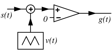
2. Mathematical model: general considerations. The ‘classical’ class-D amplifier design, without negative feedback, is illustrated in Figure 2.1. The audio input signal is denoted bys(t); generally this signal comprises a Fourier spectrum in the audible range up to 20kHz. This audio signal is added to a triangular carrier wave v(t), with periodT, that satisfies
v(t) =
1−4tT for 0≤t < T 2
−3 +4t T for
T
2 ≤t < T, (2.1)
andv(t+T) =v(t) for allt. Thusv(nT) = 1 andv((n+12)T) =−1, for any integer n, andv(t) is piecewise linear between these two values. It will be significant for the analysis that follows that ifω is a typical audio frequency thenωT 1. The main circuit element is a comparator, which compares the voltage at its noninverting input (denoted by a ‘+’ in the figure) with the voltage at its inverting input (denoted by a ‘−’), and gives an outputg(t) that satisfies
g(t) =
+1 ifs(t) +v(t)>0
−1 ifs(t) +v(t)<0. (2.2)
Note that the output voltages have been normalized to±1: furthermore, we assume throughout this paper that −1< s(t)<1 for all t. The switching times of g(t) are thus governed by s(t) +v(t) = 0; we denote the switching times from +1 to −1 by t =nT +αn, with the reverse switchings at times t =nT +βn. For the ‘classical’ design in Figure 2.1 these switching times are governed by
0< αn= T
4 (1 +s(nT+αn))< T
2 < βn= T
s(t)
+
−
+
0
v(t)
[image:3.595.163.348.91.179.2]g(t)
Fig. 2.1. ‘Classical’ class-D amplifier (without negative feedback). The audio input signal is s(t); this is summed with a high-frequency triangular carrier wavev(t)and input to the noninverting input (+) of a comparator, whose inverting input (−) is grounded. The output of the comparator is g(t), given by (2.2).
Note that the equations in (2.3) give αn and βn only implicitly. We shall consider their solution later.
We now examine how the switching times are used in computing the component ofg(t) in the audio spectrum, i.e., the amplifier output.
2.1. Comparator outputg(t). In all class-D designs, regardless of the details, the outputg(t) takes the form
g(t) =
+1 ifnT < t < nT+αn ornT+βn< t <(n+ 1)T
−1 ifnT+αn< t < nT+βn, (2.4)
for some switching timest=nT+αn and nT+βn. Thus we may write
g(t) = 1−2
∞
X
n=−∞ Hn(t), (2.5)
where
Hn(t) =H(t−(nT+αn))−H(t−(nT+βn)), (2.6)
and whereH(t) is the Heaviside step function (H(t) = 0 fort <0 andH(t) = 1 for t >0). Note that each Hn(t) has finite support:
Hn(t) =
1 nT+αn < t < nT+βn 0 otherwise,
(2.7)
so the sum in (2.5) is well defined almost everywhere (i.e., except at the exact switching times). The corresponding Fourier transform
ˆ
g(ω)≡ 1
(2π)1/2
Z ∞ −∞
g(t)e−iωtdt (2.8)
is then
ˆ
g(ω) = (2π)1/2δ(ω)−(2π)2i1/2ω ∞
X
n=−∞
n
e−iω(nT+βn)
−e−iω(nT+αn)o.
(2.9)
A formal analysis of this expression allows us to write the outputg(t) more usefully in terms of the switching times. We begin by denoting byS the sum in (2.9). Then
S=
∞
X
n=−∞
e−iωnT e−iωβn
=
∞
X
n=−∞
e−iωnT
∞
X
m=1
1 m!(−iω)
m(βm n −αmn)
=
∞
X
m=1
1 m!(−iω)
m
∞
X
n=−∞
e−iωnT(βm n −αmn). (2.10)
Now we note that
e−iωnT(βm
n −αmn) = Z ∞
−∞
e−iωt[Bm(t)
−Am(t)]δ(t−nT) dt, (2.11)
whereA(t) andB(t) are any smooth functions that satisfy
A(nT) =αn, B(nT) =βn. (2.12)
We shall refer toA(t) andB(t) as generalized switching-time functions. Substituting (2.11) in (2.10) and using the discrete Fourier transform identity
∞
X
n=−∞
δ(t−nT) = 1 T
∞
X
n=−∞
eiωcnt
, (2.13)
whereωc= 2π/T is the carrier-wave frequency, we find
S= 1 T
∞
X
m=1
1 m!(−iω)
m
∞
X
n=−∞
Z ∞ −∞
e−i(ω−nωc)t[Bm(t)
−Am(t)] dt
= (2π)
1/2
T
∞
X
m=1
1 m!(−iω)
m
∞
X
n=−∞
h ˆ
Bm(ω−nωc)−Aˆm(ω−nωc) i
. (2.14)
Here ˆAm and ˆBm are, respectively, the Fourier transforms ofAm andBm.
Now we use the separation of time scales between the audio signal and the carrier wave to generate a simpler approximation to this expression forS. We begin by noting that since the signal s(t) varies only slowly over a single period of the carrier wave, the switching times αn and βn vary only slowly with n. Thus we assume thatA(t) and B(t) are chosen to vary only on the relatively slow time scale of the signal and contain no components that vary on the shorter time scale of the carrier wave. (Of course, in practice this ‘bandwidth limiting’ is only approximate.) The upshot of this assumption is that we take into account only the term n= 0 in the sum in (2.14); then, with this approximation,
S =(2π)
1/2
T
∞
X
m=1
1 m!(−1)
m(iω)mhBˆ
m(ω)−Aˆm(ω) i
. (2.15)
Correspondingly, from (2.9) it follows that
ˆ
g(ω) = (2π)1/2δ(ω) + 2 T
∞
X
m=1
1 m!(−1)
m(iω)m−1hBˆ
m(ω)−Aˆm(ω) i (2.16)
and hence, upon inverting the Fourier transform, we obtain for the component ofg(t) in the audio spectrum (cf. [4, 5])
ga(t) = 1 + 2 T
∞
X
m=1
1 m!(−1)
mdm
−1
dtm−1[B
m(t)
This expression applies regardless of the details of the class-D amplifier design: the differences between the various designs lie in the specific relationships between the generalized switching-time functions and the signals(t); these correspondingly result in different audio outputsga(t).
2.1.1. Discussion. The infinite sum in (2.17) should, of course, be viewed with some caution, given the approximations underlying it. Even if A(t) and B(t) are signals whose frequency spectra lie entirely within the audio range, the powers Am and Bm include successively higher frequencies in their spectra. For example, if A and B are pure sinusoidal signals, each with frequency ω, thenAm andBm involve frequencies up tomω. For sufficiently largem, when|ωc∓mω|lies in the audio range, terms withn=±1 must be included in the sum (2.14), rendering inappropriate our assumption that only terms withn= 0 contribute to the output audio spectrum (for larger values ofm, additional values ofnalso become relevant). However, in the anal-ysis that follows we shall consider only the first few terms in (2.17), because these are sufficient to determine the principal distortion characteristics of the amplifier designs, hence for our purposes the difficulty with large values ofmin (2.17) is immaterial.
2.2. Alternative expression forga(t). This section may be omitted by readers interested only in the class-D amplifier designs with negative feedback, since it is primarily of importance for the ‘classical’ design without feedback, in which case we shall see below that the equations governingA(t) andB(t) take the form
A(t) = ¯A(t+A(t)), B(t) = ¯B(t+B(t)), (2.18)
for some functions ¯A and ¯B. Clearly some conditions must be imposed upon A(t) andB(t) in order that (2.18) defines ¯Aand ¯B uniquely; it is sufficient thatA(t) and B(t) should vary sufficiently slowly, i.e., |A0
(t)|<1 and|B0
(t)|<1 (cf. [5]). It then proves useful to introduce ‘warped times’
tA=t+A(t), tB=t+B(t), (2.19)
so that
tA=t+ ¯A(tA), tB =t+ ¯B(tB). (2.20)
Now to obtain a simpler expression forga(t), we note from the definition of the Fourier transform (2.8) and (2.15) thatS may be written as
S= 1 T
∞
X
m=1
(−iω)m m!
Z ∞ −∞
[Bm(t)−Am(t)]e−iωtdt, (2.21)
and hence, provided the order of the summation and integration may be interchanged,
S= 1 T
Z ∞ −∞
∞
X
m=1
(−iω)m m! [B
m(t)
−Am(t)]e−iωtdt
= 1 T
Z ∞ −∞
e−iω(t+B(t))
−e−iω(t+A(t))dt,
(2.22)
from which it follows that
iωg(ω) =ˆ 2 T
1 (2π)1/2
Z ∞ −∞
e−iω(t+B(t))
= 2 T
1 (2π)1/2
Z ∞
−∞
e−iωtB dt
dtB dtB−
Z ∞ −∞
e−iωtA dt
dtA dtA
= 2 T
iω (2π)1/2
Z ∞
−∞
e−iωtB
t(tB) dtB− Z ∞
−∞
e−iωtA
t(tA) dtA
. (2.23)
Thus, by inverting the Fourier transform, we find that
ga(t) =Ca+ 2
T [gA(t) +gB(t)], (2.24)
where Ca is a constant of integration, gA(tA) = −t(tA) and gB(tB) = t(tB). From (2.20),t(tA) =tA−A(t¯ A) andt(tB) =tB−B(t¯ B). Thus
gA(tA) =−tA+ ¯A(tA), gB(tB) =tB−B(t¯ B), (2.25)
or, equivalently,
gA(t) =−t+ ¯A(t), gB(t) =t−B(t),¯ (2.26)
so that, finally, we obtain from (2.24) and (2.26)
ga(t) = 1 + 2 T
¯
A(t)−B(t)¯ . (2.27)
The constant of integrationCa= 1 has been fixed by noting that for zero input signal (s(t)≡0) it follows from (2.2) thatga(t)≡0, while ¯A(t)≡T /4 and ¯B(t) ≡3T /4. Thus when the problem for the generalized switching times is of the form (2.18), the audio output takes a particularly simple form, which does not appear to have been noted previously.
2.3. ‘Classical’ class-D amplifier. For the ‘classical’ class-D amplifier illus-trated in Figure 2.1, we find from (2.3) and (2.12) that
A(nT) = T
4 [1 +s(nT +A(nT))], B(nT) = T
4 [3−s(nT+B(nT))]. (2.28)
It is then straightforward to extend this definition ofA(t) andB(t) appropriately to other times by globally mappingnT7→tin (2.28). Then in view of (2.18) and (2.27) it follows that
ga(t) = 1 + 2 T
T
4 [1 +s(t)]− T
4 [3−s(t)]
=s(t). (2.29)
Thus (as is well known [1, 4, 5]) this amplifier gives no distortion to the signal (given the modeling assumptions).
g(t)
+
+
−
+
k
x
dt
−c
∫
0
s(t)
h(t)
[image:7.595.129.388.75.188.2]v(t)
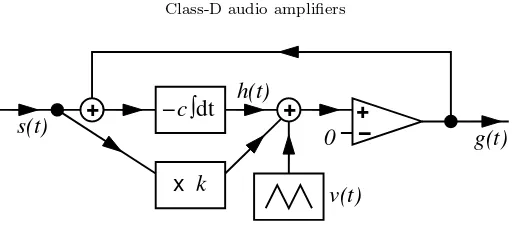
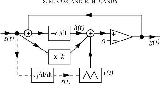
Fig. 3.1. Class-D amplifier with negative feedback. The signal s(t)is fed into a device that multiplies it by a constant k, and also into an integrator, whose output we denote byh(t). The output of the integrator and the multiplier are summed, together with a high-frequency triangular carrier wavev(t), and input to the noninverting input of a comparator whose inverting input is grounded. The output of the comparator isg(t).
3. Class-D amplifier with negative feedback. With negative feedback, the basic class-D amplifier design is illustrated in Figure 3.1.
In analysing the amplifier design, we find it convenient to introduce f(t), the integral of the input signal, defined by f0
(t) = s(t); the constant of integration in determining f(t) uniquely is not important in what follows. The triangular carrier wavev(t) again satisfies (2.1) and the periodicity conditionv(t+T) =v(t) for allt. The outputg(t) of the comparator now satisfies
g(t) =
+1 ifh(t) +ks(t) +v(t)>0
−1 ifh(t) +ks(t) +v(t)<0. (3.1)
Finally, the integrator output is given by
h(t) =−c Z t
g(τ) +s(τ) dτ. (3.2)
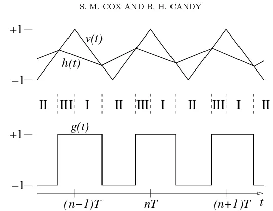
The time constantcis such thatcT =O(1). Since−1< s(t)<1,h(t) alternately in-creases and dein-creases, asg(t) is, respectively, negative and positive. The relationships between v(t), g(t) and h(t) are illustrated in Figure 3.2. We note that for illustra-tive purposes the figure shows h(t) as a piecewise linear function of time, which is appropriate only for a constant input signal; otherwiseh(t) has a slight nonlinearity.
3.1. Analysis of the model. We analyze the model by first constructing a system of nonlinear implicit difference equations for the switching timesαn and βn. To do so, we consider a time intervalnT < t <(n+ 1)T. Referring to the waveform in Figure 3.2, we see that at the start and end of this interval, h(t) is decreasing; in between,h(t) is increasing. We define three subintervals:
I: nT < t < nT+αn h0(t)<0 [g(t) = 1]; II: nT+αn < t < nT+βn h0(t)>0 [g(t) =−1]; III: nT+βn< t <(n+ 1)T h0(t)<0 [g(t) = 1], (3.3)
and consider each in turn.
Subinterval I. By integrating (3.2) we find
III
v(t)
h(t)
−1
+1
−1
+1
(n−1)T
nT
(n+1)T t
g(t)
I
II
I
II
I
II
III
[image:8.595.118.387.73.281.2]II
III
Fig. 3.2. Diagram showing relationships betweenv(t), g(t)andh(t)for the class-D amplifier with negative feedback. Note that, although h(t) is here drawn as piecewise linear, it is in fact nonlinear for any nontrivial input signal s(t). The subintervals I, II and III are indicated, as defined in (3.3).
According to (3.1), the value ofαn is defined by
h(nT+αn) +ks(nT+αn) +v(nT +αn) = 0, (3.5)
that is,
h(nT)−c[f(nT+αn)−f(nT)]−cαn+ks(nT+αn) + 1−4αn T = 0. (3.6)
Subinterval II. By integrating (3.2) and enforcing continuity of h(t) at time t=nT+αn, we find
h(t) =h(nT)−c[f(t)−f(nT)]−cαn+c(t−nT−αn). (3.7)
From (3.1), the value ofβn is defined by
h(nT+βn) +ks(nT+βn) +v(nT+βn) = 0, (3.8)
that is,
h(nT)−c[f(nT+βn)−f(nT)] +c(βn−2αn) +ks(nT+βn)−3 + 4βn
T = 0. (3.9)
Subinterval III. By integrating (3.2) and enforcing continuity of h(t) at time t=nT+βn, we find
h(t) =h(nT)−c[f(t)−f(nT)] +c(βn−2αn)−c(t−nT−βn). (3.10)
For the remaining analysis, we note that at the end of this subinterval
nT
η
h(t)
t
(n+4)T
(n+3)T
(n+2)T
(n+1)T
[image:9.595.132.384.75.176.2](t)
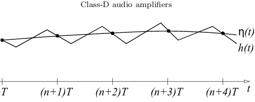
Fig. 3.3. Diagram showing relationship betweenh(t) and η(t). The two functions agree at times nT (for integers n), buth(t) varies significantly at intermediate times, whereas η is only slowly varying.
3.2. Solution of the governing equations. Our goal is to use (2.17) to de-termine the audio output of the amplifier. To do so we first need to dede-termine the switching times ofg(t). Given a signals(t), we determine these switching times, to-gether with the values of h(nT), from the coupled equations (3.6), (3.9) and (3.11), which are, so far, exact.
We first use (2.12) to substitute the generalized switching-time functions for αn andβn; the result is a system of three equations involvingA(nT),B(nT) andh(nT). These equations are readily extended to intermediate times by mappingnT 7→t:
4
T +c
A(t) = 1 +ks(t+A(t)) +η(t)−c[f(t+A(t))−f(t)], (3.12)
4
T +c
B(t) = 3−ks(t+B(t))−η(t) +c[f(t+B(t))−f(t)] + 2cA(t), (3.13)
η(t+T) =η(t)−c[f(t+T)−f(t)] +c[2B(t)−2A(t)−T]. (3.14)
Since the functionsA(t) andB(t) vary only on the time scale of the audio signal and not on that of the carrier wave, the function h(t) is replaced in these expressions by a slowly varying functionη(t) such that
η(nT) =h(nT) (3.15)
(see Figure 3.3).
Given the mild restrictions on the form of the input signals(t) and its first integral f(t), it seems unlikely that a general solution can be found to the coupled nonlinear equations (3.12)–(3.14). Furthermore, it seems unlikely that any solution will be unique, although we are unable to demonstrate nonuniqueness for the system of three equations as posed. (A suggestion of nonuniqueness comes from the following thought experiment. Suppose A(t) and B(t) are known and independent of η(t). Then the solutionη(t) to (3.14) is unique only up to the addition of a function of periodT [3]. Note that here the nonuniqueness involves high-frequency components only.)
We find that we are able to construct a solution to (3.12)–(3.14) with frequency spectrum in the audio range, as follows. The derivation is admittedly rather informal. We introduce the small parameter =ωtyp/ωc 1, where ωtyp is a typical audio
frequency component of the input. Then we note that (3.12)–(3.14) relate to variations ins, A,B andη on a time scalet=O(T), and that such variations satisfy
dn dtn =O(
We then expandA(t),B(t) andη(t) as series
A(t) =
∞
X
m=0
Am(t), B(t) =
∞
X
m=0
Bm(t), η(t) =
∞
X
m=0
ηm(t), (3.16)
where the terms in (3.16) satisfy
Am, Bm, ηm=O(m).
For all functions in (3.12)–(3.14) not evaluated at timet, we make use of Taylor expansions such as
η(t+T) =
∞
X
n=0
Tnη
(n)(t)
n! (3.17)
to write them in terms of functions and derivatives evaluated at timet.
As an aside, we note that an alternative mathematical solution may possibly be developed using the calculus of finite differences [3], where problems such as (3.14), of the form u(t+T)−u(t) =U(t), are examples of the so-called ‘summation prob-lem’. However, the added complication of (3.12) and (3.13) makes a complete explicit solution unlikely. We note, however, that (3.14) has the exact formal solution
η(t) =−cf(t) +c
∞
X
n=1
[2B(t−nT)−2A(t−nT)−T].
Some of the key terms in the various expansions are
f(t+T)−f(t) =T s(t) +1 2T
2s0
(t) +1 6T
3s00
(t) +O(3) η(t+T)−η(t) =T η0
0(t) +
T η0
1(t) +12T 2η00
0(t)
+O(3) s(t+A(t)) =s(t) +A0(t)s0(t) +12A20(t)s
00
(t) +A1(t)s0(t)+O(3)
s(t+B(t)) =s(t) +B0(t)s0(t) +12B02(t)s 00
(t) +B1(t)s0(t)+O(3)
f(t+A(t))−f(t) =A0(t)s(t) +12A20(t)s 0
(t) +A1(t)s(t)
+1 6A
3 0(t)s
00
(t) +A0(t)A1(t)s0(t) +A2(t)s(t)+O(3)
f(t+B(t))−f(t) =B0(t)s(t) +12B02(t)s 0
(t) +B1(t)s(t)
+1 6B
3 0(t)s
00
(t) +B0(t)B1(t)s0(t) +B2(t)s(t)+O(3).
In view of (2.17), we also have the expansion
ga(t) = 1− 2
T(B0−A0) + 1
T
(B02−A20) 0
−2(B1−A1)
+ 1 T −1 3(B 3 0−A30)
00
+ 2(B0B1−A0A1)0−2(B2−A2)+O(3)
(3.18)
for the audio output. With obvious notation, we write this as
ga(t) =g0(t) +g1(t) +g2(t) +O(3).
(3.19)
to (3.13) we eliminate the unknown functionη(t) and arrive at an equation that at O(n) takes the form
{4−cT[1−s(t)]}An(t) +{4 +cT[1−s(t)]}Bn(t) =Pn(t), (3.20)
where Pn(t) is known in terms of quantities calculated at previous stages in the calculation. Furthermore, (3.14) can be written in the form
Bn(t)−An(t) =Qn(t), (3.21)
where againQn(t) comprises known quantities. This system is readily solved to give
An(t) =18{Pn(t)−[4 +cT(1−s(t))]Qn(t)}, (3.22)
Bn(t) =18{Pn(t) + [4−cT(1−s(t))]Qn(t)}. (3.23)
AtO(0), we findP
0= 4T andQ0= 12T(1 +s(t)). Correspondingly,
A0= 161T(1−s(t)) [4−cT(1 +s(t))]
(3.24)
B0= 12T+161T(1 +s(t)) [4−cT(1−s(t))],
(3.25)
so the switching times approximately satisfy
αn= 161T(1−s(nT)) [4−cT(1 +s(nT))] (3.26)
βn= 12T+161T(1 +s(nT)) [4−cT(1−s(nT))]. (3.27)
Of most significance is the result, which now follows from (3.24), (3.25) and (3.18), that
g0(t) =−s(t).
(3.28)
Thus to this order there is no distortion from signal to output, apart from a sign change, which is unimportant for audio applications. However, in contrast to the ‘classical’ design, the next orders in the expansion of the audio output reveal distortion inherent in the nonlinear-feedback design. (The minus sign in (3.28) is an artifact of applying the triangular wave input to the noninverting input of the comparator; if it is instead applied to the inverting input then there is no sign change to the output.)
3.3. Amplifier output. The next steps in the calculation are algebraically cum-bersome and shed little further light on the problem, so the full details are not pre-sented here. Our primary interest lies in the audio output, and this turns out to be
ga(t) =−s(t) +1 +k c s
0
(t)
−48c12
[48(1 +k)−c2T2]s(t)−c2T2s3(t) 00+O(3). (3.29)
Note that there arises a nonlinear (cubic) distortion term; this term is to leading order independent of k, so it cannot be removed by any choice of this parameter. This nonlinear term represents the ‘intrinsic’ distortion of class-D amplifiers with negative feedback to which we have alluded above.
be removed by making an appropriate choice ofksuch that the linear terms in (3.29) form the beginnings of a Taylor series for a slightly delayed signal−s(t−(1 +k)/c). It is readily determined that the appropriate value ofksatisfies
k2= 1− 1 24c
2T2;
(3.30)
correspondingly, the audio output is then given by
ga(t) =−s(t−(1 +k)/c) +481T2 s3(t)
00
+O(3). (3.31)
Note that the delay to the output indicated here is independent of signal amplitude and frequency, and thus is entirely benign. Furthermore, (1 +k)/c is a time of the order of the carrier-wave period, so the delay to the audio signal is slight. However, the nonlinear distortion term remains.
For the specific case of a sinusoidal input signals(t) =s0sinωt, (3.29) becomes
ga(t) =−s0sinωt+ (1 +k)µs0cosωt
+ µ
2
192
192(1 +k)−(4 + 3s20)c2T2
s0sinωt+ 9c2T2s30sin 3ωt +O(µ3),
(3.32)
whereµ=O(): specifically
µ= ωT cT 1. (3.33)
We note from (3.32) that the intrinsic nonlinear distortion manifests itself through both a nonlinear influence on the amplitude of the fundamental, and the presence of a third-harmonic term.
3.4. Alternative expression forga(t). An alternative expression for the audio output may be derived as follows. First we note that the switching times for g(t) satisfy
αn= T
4 [1 +h(nT+αn) +ks(nT+αn)],
βn= T
4 [3−h(nT+βn)−ks(nT+βn)].
If we introduce two new slowly varying functionsη(t;α) andη(t;β) defined so that
η(nT+αn;α) =h(nT+αn), η(nT+βn;β) =h(nT+βn), (3.34)
then it follows from (2.29) that
ga(t) = 12[η(t;α) +η(t;β)] +ks(t). (3.35)
Although this expression does not yield a useful explicit exact formula for ga(t), it does provide an alternative means of calculating ga(t). This in turn gives us an independent check on our results, which we have used to verify expressions such as (3.29).
w(t)
+
v(t)
dt
∫
[image:13.595.107.402.72.203.2]−c
1
r(t)
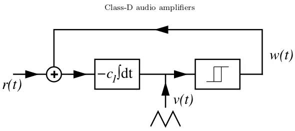
Fig. 4.1.Circuit diagram for modulation of the carrier wave. The modulation functionr(t)is input to an integrator, whose outputv(t)is input to a hysteresis loop. The outputw(t)of the last device takes the value+1once its input has reached the value +1; thereafterw(t)remains at+1, until the inputv(t) falls to−1, from which point onwardsw(t) =−1, until the inputv(t)reaches
+1again, and so on.
4. Modulation of the carrier wave. We now examine one means of eliminat-ing the ‘intrinsic distortion’ term in (3.29). The key to the technique is to modulate the carrier wave in such a way that the switching times ofg(t) are slightly altered in an appropriate fashion to counter the distortion. This technique is used successfully for distortion reduction in amplifiers manufactured by Halcro Pty Ltd (www.halcro.com).
We suppose that the carrier wave is modulated by a slowly varying input signal r(t), wherer(t) =e0
(t), for some functione(t); sincer(t) involves a first derivative, it is taken to beO(), and the modulation of the carrier wave correspondingly slight. The modulation circuit is illustrated in Figure 4.1; the full amplifier circuit is caricatured in Figure 4.2. Now the carrier wavev(t) is governed by
v(t) =−c1
Z t
w(τ) +r(τ) dτ, (4.1)
where c1 is a time constant associated with the integrator in the modulation circuit
(see Figure 4.1), and is no longer quite piecewise linear. The signal w(t) is a square wave of variable duty cycle, taking the valuesw(t) = ±1, depending on the carrier wave v(t) as follows. First, suppose that w = −1; then v is increasing. When v reaches +1,wchanges to +1 and v starts to decrease. Oncev has decreased to−1, w changes to −1; thenv starts to increase once more, until it reaches +1 again, at which point the cycle starts over.
4.1. Analysis of the model. Suppose that w(t) changes to the value w= 1 at times t = Tn, and changes to the value w = −1 at times t = Un. Then for Tn< t < Un, w(t) = 1 and hence
v(t) = 1−c1[e(t)−e(Tn)]−c1(t−Tn). (4.2)
ForUn< t < Tn+1, w(t) =−1 and
v(t) =−1−c1[e(t)−e(Un)] +c1(t−Un). (4.3)
The time constant c1 (determined below) is such that c1T = O(1). Constants of
integration have been chosen so that each of these expressions gives the correct value forv(t) at the start of each time interval. Imposing the appropriate value forv(t) at the end of each time interval then gives the two conditions
c1[e(Un)−e(Tn)] +c1(Un−Tn) = 2 (4.4)
1
+
+
−
+
k
x
dt
−c
∫
0
h(t)
g(t)
v(t)
s(t)
r(t)
d/dt
[image:14.595.128.385.77.215.2]c
1−Fig. 4.2. Class-D amplifier with negative feedback and modulation of the carrier-wave sym-metry. Note that the entire circuitry of Figure 4.1 is represented by the single box marked ‘v(t)’. The appropriate modulation signalr(t) =c−11s0(t)is indicated on the diagram, as determined in
Section 4.1.2.
For the special case in whichr(t)≡r0 is constant, the carrier wavev(t) is
time-periodic, with period of oscillation
T = 4
(1−r2 0)c1 ∼
4 c1
(1 +r20).
Furthermore, in this case
Un−Tn= 2 (1 +r0)c1 ∼
2
c1(1−r0).
Note that T is in general increased by the presence of a nonzero modulation signal (i.e., the frequency of the carrier wave is reduced). In what follows, we shall require corrections to the carrier-wave due to modulation only up to O(), and thus, since r2 =O(2), we may take T as fixed. Then the time constant c
1 must be chosen so
that
c1= 4
T. (4.6)
With this approximation, it turns out that we may consistently calculate terms inga(t) up toO(2), which is sufficient to determine the effects of carrier-wave modulation on
the amplifier’s distortion characteristics.
If we write the times at which the slope of the triangular wave changes as
Tn=nT+an, Un=nT+bn, (4.7)
where 0< an < bn< T, then these times are now governed by
0 =h(nT)−c[f(nT+αn)−f(nT)]−cαn+ks(nT+αn) + 1−c1[e(nT+αn)−e(nT+an)]−c1(αn−an) (4.8)
0 =h(nT)−c[f(nT+βn)−f(nT)] +c(βn−2αn) +ks(nT +βn)
−1−c1[e(nT+βn)−e(nT+bn)] +c1(βn−bn), (4.9)
The solution technique is just as with no modulation. Again we seek slowly varying generalized switching times A(t) and B(t) of the output g(t), but now we need two further slowly varying functions,C(t) andD(t), such that
C(nT) =an, D(nT) =bn. (4.10)
The equations to be solved arise from (3.14), (4.4), (4.5), (4.8) and (4.9), and are
c1[e(t+D(t))−e(t+C(t))] +c1(D(t)−C(t)) = 2
(4.11)
−c1[e(t+T+C(t+T))−e(t+D(t))] +c1(T+C(t+T)−D(t)) = 2
(4.12)
η(t)−c[f(t+A(t))−f(t)]−cA(t) +ks(t+A(t)) + 1−c1[e(t+A(t))−e(t+C(t))]−c1(A(t)−C(t)) = 0
(4.13)
η(t)−c[f(t+B(t))−f(t)] +c(B(t)−2A(t)) +ks(t+B(t))
−1−c1[e(t+B(t))−e(t+D(t))] +c1(B(t)−D(t)) = 0
(4.14)
η(t+T)−η(t) +c[f(t+T)−f(t)]−c[2B(t)−2A(t)−T] = 0. (4.15)
As with the simpler case of an unmodulated carrier wave, we expand all unknown functions (hereA, B, C, D andη) as series, as in (3.16), and solve in succession for the terms in these series at the first few orders.
4.1.1. Discussion. When expanded, (4.11) and (4.12) each yield at O(1) and atO() identical equations, of the forms
D0(t)−C0(t) =12T, D1(t)−C1(t) =−12T r(t),
(4.16)
respectively. The fact that only the difference between the times C and D may be determined partly reflects an arbitrariness in the time origin for the circuit that generates the carrier wave. However, if we continue to the next order we find that the two equations for D2(t)−C2(t) are in fact inconsistent, reflecting the more serious
limitation imposed upon the analysis by our assumption that the mean carrier-wave period is unaltered by the modulation. Fortunately, a consistent calculation of C andD up to termsC1andD1 proves sufficient to determine the audio output of the
amplifier up tog2, which allows us to calculate the elimination of the distortion.
4.1.2. Elimination of the distortion. We find the audio output to be ga(t) =−s(t) +1 +k
c s
0
(t)
−3c12 1c2
3c1c2(rs2)0+3(1 +k)c21−c2
s00
−3c1c2r0−c2(s3)00 +O(3),
(4.17)
wherec1is given by (4.6). There are two nonlinear distortion terms in this expression,
proportional to (rs2)0
and (s3)00
. If we setr=νs0
(t), we may eliminate both of them by choosingν = 1/c1=T /4. Then
ga(t) =−s(t) +1 +k c s
0
(t)−12c12
12(1 +k)−c2T2 s00
(t) +O(3). (4.18)
Thus all nonlinear distortion is removed, at least to the order calculated. A key result of the present analysis is that the appropriate modulation of the carrier wave is through a derivative of the input signal; this is in fact the method used in practice.
Now if we choosek2= 1−1 6c
2T2, then the audio output is of the form
ga(t) =−s(t−(1 +k)/c) +O(3), (4.19)
k
+ −c ∫dt
− + +
S/H s(t)
h(t)
g(t) 0
v(t) p(t)
[image:16.595.111.403.74.203.2]x
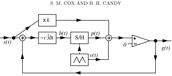
Fig. 5.1. ‘Sample-and-hold’ class-D amplifier with negative feedback. The sample-and-hold (‘S/H’) device is synchronized with the carrier-wave generator and gives an outputp(t)equal to its inputh(t)sampled at timest=nT andt= (n+1
2)T. Thus fornT ≤t <(n+12)T,p(t) =h(nT); correspondingly, for(n+1
2)T ≤t <(n+ 1)T,p(t) =h((n+12)T).
5. ‘Sample-and-hold’ class-D amplifier with negative feedback. Modu-lation of the carrier wave is not the only means by which the leading-order nonlinear distortion can be removed from class-D amplifiers with negative feedback. We now describe an alternative means of eliminating this distortion, without carrier-wave mod-ulation. This alternative amplifier design has also been constructed, in prototype, by Halcro Pty Ltd, and is illustrated in Figure 5.1. Now there is no modulation of the carrier-wave symmetry.
Now the output of the integrator inputs to a sample-and-hold device, which samples h(t) at times t = nT and (n+ 1
2)T; its output p(t) is then a
piecewise-constant function. For nT ≤ t < (n+ 1
2)T, p(t) takes the value h(nT), while for
(n+ 1
2)T ≤ t < (n+ 1)T, p(t) takes the value h((n+ 1
2)T). Aside from this new
feature, most details of the model remain essentially unchanged. The triangular wave v(t) again satisfies (2.1) andv(t+T) =v(t) for all t. The output g(t) of the com-parator is now +1 if p(t) +ks(t) +v(t)>0 and −1 if the inequality is reversed; the switching times thus satisfy
p(nT+αn)+ks(nT+αn)+v(nT+αn) = 0, p(nT+βn)+ks(nT+βn)+v(nT+βn) = 0.
The integrator outputh(t) is again given by (3.2). In any intervalnT < t <(n+ 1)T, there are three subintervals, as in (3.3); we describe these below. The analysis is somewhat simplified by the sampling.
Subinterval I. By integrating (3.2) we find thath(t) is again given by (3.4), but now the value ofαn is defined by
p(nT+αn) +ks(nT+αn) +v(nT+αn) = 0, (5.1)
that is,
h(nT) +ks(nT +αn) + 1−4αn T = 0. (5.2)
Subinterval II. By integrating (3.2) we again find (3.7) forh(t); the value ofβn is defined by
p(nT +βn) +ks(nT+βn) +v(nT +βn) = 0, (5.3)
that is,
h((n+1
2)T) +ks(nT+βn)−3 +
Subinterval III. By integrating (3.2) we find (3.10) for h(t); it follows that h((n+ 1)T) is again given by (3.11).
5.1. Solution of the governing equations. The three governing equations are now
4
Tαn= 1 +ks(nT+αn) +h(nT), (5.5)
4
Tβn= 3−ks(nT+βn)−h((n+
1 2)T),
(5.6)
h((n+ 1)T) =h(nT)−c[f((n+ 1)T)−f(nT)] +c(2βn−2αn−T). (5.7)
Furthermore, by considering Subinterval II, we find that
h((n+1
2)T) =h(nT)−c[f((n+ 1
2)T)−f(nT)] +c
T
2 −2αn
. (5.8)
As above, we introduce the slowly varying functions A(t), B(t) and η(t), which now satisfy
4
TA(t) = 1 +ks(t+A(t)) +η(t), 4
TB(t) = 3−ks(t+B(t))−η(t) +c[f(t+T /2)−f(t)]−c[T /2−2A(t)], η(t+T) =η(t)−c[f(t+T)−f(t)] +c[2B(t)−2A(t)−T],
and solve these equations at successive orders in . The audio output is eventually found to be
ga(t) =−s(t) + 1 +k
c s
0
(t)
+ 1
96c2(4−cT)
c3T3−(28 + 24k)c2T2+ 192(1 +k)cT −384(1 +k) s(t)
+ [cT −4(1 + 2k)]c2T2s3(t) 00
+O(3).
(5.9)
Now the nonlinear distortion term proportional to (s3)00
may be removed from this expression by choosing
k=−1 2 +
1 8cT,
(5.10)
in which case
ga(t) =−s(t) +4 +cT 8c s
0
(t)−24−c 2T2
48c2 s 00
(t) +O(3). (5.11)
Once the nonlinear distortion term has been so removed, we may similarly remove linear distortion, so that the audio output only suffers a slight delay, i.e.,
ga(t) =−s(t−18(4 +cT)/c) +O(3),
5.2. Alternative means of sampling. Suppose now that the sampling is car-ried out only at timest=nT(i.e., not also at timest= (n+1
2)T). Then the equations
to be solved forA(t),B(t) andη(t) are somewhat simplified:
4
TA(t) = 1 +ks(t+A(t)) +η(t), (5.12)
4
TB(t) = 3−ks(t+B(t))−η(t), (5.13)
η(t+T)−η(t) =−c[f(t+T)−f(t)] +c[2B(t)−2A(t)−T]. (5.14)
The audio output is, correspondingly, found to be
ga(t) =−s(t) + 1 +k
c s
0
(t) + 1 96c2
−(2k+ 1)c2T2(3s2(t) +s3(t))00
+
−c2T2−6(1 +k)c2T2+ 48(1 +k)cT−96(1 +k) s00
(t) . (5.15)
In view of the asymmetrical sampling, there are now second and third harmonics at O(2), but these cansimultaneouslybe removed by choosing
k=−12.
If this choice is made, thenga(t) becomes
ga(t) =−s(t) + 1 2cs
0
(t)−24c12
12−6cT +c2T2 s00
(t) +O(3). (5.16)
This is a delayed version of the original signal (ga(t) = −s(t−12c) +O(3)) if the choicecT = 3 is made.
6. A new class-D amplifier, with reduced distortion. We now describe a third modification to the standard negative-feedback class-D amplifier, which elim-inates the intrinsic distortion at O(2). While the two designs described above in
Sections 4 and 5 were developed first on physical principles and subsequently here modelled mathematically, this new design arose as a consequence of the mathematical models described herein. Prototypes do indeed enjoy significant distortion reduction. To see how this new design is derived, we consider adding to the noninverting input of the comparator a functionF(t) such thatF(t) is constant over each interval nT ≤t <(n+ 1)T. At present the values taken by this function over each interval are arbitrary; we shall compute the effects of F(t) on the audio output spectrum, then choose it so as to cancel out the intrinsic distortion.
With this additional design feature, the audio output of the amplifier is found to be
ga(t) =−s(t) +1
c [(1 +k)s(t) +θ(t)]
0
−48c12
48 + 24cT−3c2T2 θ0
(t) + 48(1 +k)−c2T2 s0
(t)
+ 3c2T2[θ(t)−s(t)]0
s2(t) 0
+O(3),
(6.1)
whereθ(t) is a slowly varying function that agrees withF(t) at timest=nT. The last line of (6.1) represents the nonlinear distortion, and it is clear that this component can be eliminated by choosing
and henceθ(t) =s(t). Fortunately, no further distortion is introduced by this choice forF(t), and we have
g(t) =−s(t) +2 +k c s
0
(t)−12(2 +k) + 6cT −c 2T2
12c2 s
00
(t) +O(3), (6.3)
which is free from any nonlinear distortion. As in the other models above, it is possible to choose k so that the output is, to the order calculated, a delayed version of the input signal, and suffers no further distortion beyond the slight delay.
7. Nonlinearity in the carrier wave. We now consider one way in which imperfect electronic components can introduce distortion into the output. Specifically, we note that it is difficult in practice to generate a high-frequency triangular carrier wave whose slopes are precisely linear. In general the wave comprises sections of exponential functions, which approximate very closely the desired piecewise-linear profile [6]. For instance, let us suppose that instead of (2.1) we have for the carrier wave
v(t) =
1−2(e
t/t0 −1)
eT /2t0−1 ≡v1(t) for 0≤t <
T 2
−1 +2(e
(t−T /2)/t0 −1)
eT /2t0−1 ≡v2(t) for
T
2 ≤t < T, (7.1)
andv(t+T) =v(t) for allt. Note that the piecewise-linear profile of (2.1) is recovered ast0/T → ∞.
7.1. ‘Classical’ class-D amplifier design. Let us first consider the effects of carrier-wave nonlinearity on the ‘classical’ class-D amplifier design, without negative feedback. Here switching ofg(t) takes place wheneverv(t) +s(t) = 0, i.e., when
v1(nT+αn) +s(nT+αn) = 0 or v2(nT+βn) +s(nT+βn) = 0. (7.2)
These expressions are readily rearranged to give implicit equations for the switching times:
αn=t0log
n 1 + 1
2[1 +s(nT+αn)](e
T /2t0 −1)o, (7.3)
βn= 12T+t0log
n
1 +12[1−s(nT+βn)](eT /2t0 −1) o
. (7.4)
It now follows readily from (2.27) that the audio output is
ga(t) =2t0 T log
1 +12[1 +s(t)](eT /2t0 −1) 1 +12[1−s(t)](eT /2t0−1).
(7.5)
(It is straightforward from this expression to check thatg(t)∼s(t) ast0/T → ∞, in
accordance with (2.29).) Since it follows by Taylor expansion that
ga(t)∼ 4t0
T
∞
X
n=0
1 2n+ 1
(eT /2t0
−1)s(t) eT /2t0+ 1
2n+1 , (7.6)
we may in principle compute the audio spectrum, for instance, due to a sinusoidal inputs(t).
We contrast the result here, where ga 6≡s, and there is nonlinear distortion of O(T /t0), with that for a perfectly piecewise-linear carrier wave, where there is no
7.2. Class-D amplifier with negative feedback. We now consider the ef-fects of carrier-wave nonlinearity on the class-D amplifier with negative feedback (as illustrated in Figure 3.1). It turns out that, providedT /t01, then to leading order
in the nonlinearity, the outputga(t) as given by (3.29) is augmented by a term of the form
T2 16t0
s3(t)−s(t)0
. (7.7)
Note that the nonlinear distortion term here (proportional to (s3)0
) can be thought of as having a different phase to that inherent in the basic amplifier design (proportional to (s3)00
), so one cannot be used to cancel the other.
However, if we modify the design by adding to the comparator input a quantity
− 1
ct0
h(t) (7.8)
sampled at times
t=nT and (n+1 2)T,
(7.9)
in addition to the modification proposed in Section 6, then the third-harmonic dis-tortion term due to the carrier wave nonlinearity is cancelled, and
ga(t) =−s(t) +c−1(2 +k)s0(t) +c−2
−1
12 12(2 +k) + 6cT−c 2T2
s00
(t) +t−1
0 (2 +k)s 0
(t)
+O(3). (7.10)
With an appropriate choice fork, this expression is essentially just a slightly delayed version of the input signal, i.e.,
ga(t) =−s(t−t1) +O(3).
(7.11)
To achieve this simplification we take
k=−1 + 1 +cT−1 6c
2T21/2 ,
then the delay is
t1=2 +k
c
1 + 1 ct0
.
To the order calculated, there is no further distortion; the delay computed here is independent of the signal amplitude or frequency.
intrinsic distortion has been proposed, on the basis of the mathematical models devel-oped, which involves the use of a sample-and-hold device, but in a manner different to that in the existing design.
One of us (BHC) has tested all three designs (i.e., those described in Sections 4, 5 and 6) in prototype and found them all to achieve significant reduction in harmonic distortion. The two designs involving a sample-and-hold unit are found not to work as well in practice as the carrier-wave modulation system, and are more expensive to produce. The carrier-wave modulation design is the basis of a successful commercial amplifier manufactured by Halcro Pty Ltd.
It should be noted that the models developed here do not reflect a range of important practical issues, such as the noise and stability characteristics of the de-signs, nor their electromagnetic emissions. The models assume perfect components, an assumption that has particularly significant shortcomings in relation to sample-and-hold devices, for which the errors are relatively severe (in comparison, say, with integrators).
The models developed in this paper appear to be the first to provide an in-depth mathematical treatment of class-D amplifiers with negative feedback, and should be capable of extension to more complicated designs that reflect more accurately actual audio amplifiers.
REFERENCES
[1] H. S. Black,Modulation theory, van Nostrand, New York, 1953.
[2] P. H. Mellor, S. P. Leigh and B. M. G. Cheetham,Reduction of spectral distortion in class D amplifiers by an enhanced pulse width modulation sampling process, IEE Proc.-G, 138 (1991), pp. 441–448.
[3] L. M. Milne–Thomson,The calculus of finite differences, Macmillan, London, 1933.
[4] C. Pascual, Z. Song, P. T. Krein, D. V. Sarwate, P. Midya and W. J. Roeckner, High-fidelity PWM inverter for digital audio amplification: spectral analysis, real-time DSP im-plementation, and results, IEEE Trans. Power Electronics, 18 (2003), pp. 473–485. [5] Z. Song and D. V. Sarwate,The frequency spectrum of pulse width modulated signals, Signal
Processing, 83 (2003), pp. 2227–2258.
[6] M. T. Tan, J. S. Chang, H. C. Chua and B. H. Gwee,An investigation into the parameters affecting total harmonic distortion in low-voltage low-power Class-D amplifiers, IEEE Trans. Circuits and Systems I, 50 (2003), pp. 1304–1315.