HEATING EFFECTS FROM DRIVEN TRANSVERSE AND ALFV ´EN WAVES IN CORONAL LOOPS
Mingzhe Guo,1, 2 Tom Van Doorsselaere,2 Kostas Karampelas,2Bo Li,1 Patrick Antolin,3 and Ineke De Moortel3
1Institute of Space Sciences, Shandong University, Weihai 264209, China
2Centre for mathematical Plasma Astrophysics, Department of Mathematics, KU Leuven, 3001 Leuven, Belgium 3School of Mathematics and Statistics, University of St. Andrews, St. Andrews, Fife KY16 9SS, UK
(Received; Revised; Accepted)
ABSTRACT
Recent numerical studies revealed that transverse motions of coronal loops can induce the Kelvin-Helmholtz Insta-bility (KHI). This process could be important in coronal heating because it leads to dissipation of energy at small spatial-scale plasma interactions. Meanwhile, small amplitude decayless oscillations in coronal loops have been discovered recently in observations of SDO/AIA. We model such oscillations in coronal loops and study wave heating effects, considering a kink and Alfv´en driver separately and a mixed driver at the bottom of flux tubes. Both the transverse and Alfv´en oscillations can lead to the KHI. Meanwhile, the Alfv´en oscillations established in loops will ex-perience phase mixing. Both processes will generatesmall spatial-scale structures, which can help the dissipation of wave energy. Indeed, we observe the increase of internal energy and temperature in loop regions. The heating is more pronounced for the simulation containing the mixed kink and Alfv´en driver. This means that the mixed wave modes can lead to a more efficient energy dissipation in the turbulent state of the plasma and that the KHI eddies act as an agent to dissipate energy in other wave modes. Furthermore, we also obtained forward modelling results using the FoMo code. We obtained forward models which are very similar to the observations of decayless oscillations. Due to the limited resolution of instruments, neither Alfv´en modes nor thefine structuresare observable. Therefore, this numerical study shows that Alfv´en modes probably can co-exist with kink modes, leading to enhanced heating.
Keywords: magnetohydrodynamics (MHD) — Sun: corona — Sun: magnetic fields — waves
1. INTRODUCTION
A rich variety of MHD oscillations and waves have been observed in the highly structured solar atmosphere(for recent reviews, e.g., Nakariakov & Verwichte 2005; De Moortel & Nakariakov 2012;Nakariakov et al. 2016; Jess et al. 2015). They may play an important role in coronal heating because of their capability of carrying energy (e.g., Taroyan & Erd´elyi 2009; Parnell & De Moortel 2012). In fact, analytical studies to reveal the various wave properties in magnetic structures date back to 1970s (Zajtsev & Stepanov 1975; Wentzel 1979). In 1999, the first imaging observation of kink waves in active region loops was obtained by the Transition Region and Coronal Explorer (TRACE,Aschwanden et al. 1999;Schrijver et al. 1999;Nakariakov et al. 1999). Since then, a large number of transverse waves were discovered in the solar atmosphere by modern instruments(e.g.,Nakariakov & Verwichte 2005; Verwichte et al. 2005;Aschwanden 2006;Tomczyk & McIntosh 2009), not only in coronal loops (see Ruderman & Erd´elyi 2009, for a recent review),but in chromospheric spicules and mottles (e.g.,De Pontieu et al. 2007;He et al. 2009;Morton et al. 2012;Kuridze et al. 2012,2013), large prominences(e.g.,Arregui et al. 2012), polar plumes(e.g.,Gupta et al. 2010), and coronal streamers(e.g.,Chen et al. 2010,2011;Kwon et al. 2013).
The observed large-amplitude transverse oscillations generally undergo rapid damping in a couple of periods (Nakari-akov et al. 1999;Aschwanden et al. 2002;Goddard et al. 2016). Such damping is usually attributed to resonant absorp-tion (Hollweg & Yang 1988;Goossens et al. 1992,2002) or phase mixing (Soler & Terradas 2015). The kink oscillations transfer into local Alfv´en modes when the kink frequency matches the local Alfv´en frequency, therefore the transverse motion has an apparent decay. This process is usually expected to happen in an inhomogeneous layer near the loop boundary. On the other hand,Soler & Terradas(2015) considered the phase mixing process simultaneously, which is responsible for the wave energy transfer fromlarge spatial-scale structurestosmall scale plasma interactions. The real dissipation of wave energy atsuch small structuresrelies on resistivity and viscosity (Ofman et al. 1994, 1998).
Recent simulations of transverse waves in coronal loops revealed that the Kelvin-Helmholtz instability occurs near the boundary of loops (Terradas et al. 2008; Antolin et al. 2014, 2017; Magyar et al. 2015; Karampelas et al. 2017; Howson et al. 2017a,b). The instability is generated due to the strong shear motions near the loop edges. Meanwhile, the generation of azimuthal Alfv´en waves at resonant layers increases the velocity shear with the external plasma, which can also enhance the instability and make the systems more unstable. Antolin et al.(2014) revealed that even a small-amplitude (∼ 3km s−1) kink oscillation can lead to such an instability. The importance of this Transverse
Wave Induced Kelvin-Helmholtz (TWIKH) instability (Antolin et al. 2014,2017) is that it generates turbulentsmall structures. This makes the wave energy dissipate much more easily in thesmall scale structuresin the presence of transport coefficients or kinetic effects. This is probably a crucial process for coronal heating(Karampelas et al. 2017; Howson et al. 2017a).
Due to their incompressibility, Alfv´en waves are not easily detected by imaging instruments in the solar atmosphere. Their torsional motions would cause spectral line broadening, making them detectable to spectrographs (Zaqarashvili 2003). Jess et al.(2009) reported the torsional Alfv´en waves in the chromosphere, using the H-α line in Solar Optical Universal Polarimeter (SOUP) of SST. However, the corresponding coronal observations remain unclear. Theoretically, Alfv´en waves can be easily generated from the lower atmosphere (Muller et al. 1994; Beli¨en et al. 1999). Vranjes et al.(2008) claimed that the wave energy flux through the photosphere becomes orders of magnitude smaller when considering the effects of partial ionization and collisions. However, the fast waves transfer their energy to upgoing Alfv´en waves in the conversion region. The process is analogous to the resonant absorption mentioned above, making the Alfv´en flux increase significantly in the lower atmosphere (Khomenko & Cally 2012; Cally & Moradi 2013;Grant et al. 2018). Similar to kink waves, the energy dissipation is an important issue. Heyvaerts & Priest (1983) claimed that phase mixing occurs between different magnetic surfaces when Alfv´en waves propagate in the non-uniform magnetic structures. Recent work byPagano et al.(2018) found that heating from phase mixing of Alfv´en modes in coronal loops with multi-harmonic oscillations is small. However, the Kelvin-Helmholtz instability can be induced for standing modes eventually due to the strong, localised velocity shear. Such small turbulent structures induced through the instability can help wave energy dissipate more easily.
such undamped regimes as the response of loops to external continuous drivers. Antolin et al.(2016) explained such oscillations as combined effects of periodic brightening of TWIKH rolls and the limited resolution of instruments. Nakariakov et al. (2016) proposed that these decayless oscillations were caused by interaction of loops with quasi-steady flows as self-oscillations. Very recently, Karampelas et al. (2017); Karampelas & Van Doorsselaere (2018) simulated such decayless transverse oscillations as coronal loops driven by transverse motions.
In this article, we aim to simulate such driven oscillations and study the heating effects, considering a mixed kink and Alfv´en driver at one footpoint of a loop. Matsumoto & Shibata(2010) claimed that turbulent photospheric motions can be observed by Hinode/SOT, therefore it is reasonable to expect mixed motions at the footpoints of loops. The mixed processes of KHI, resonant absorption and phase mixing will greatly influence the heating effects. Meanwhile, the decayless oscillations are ubiquitous in coronal loops, so it is worthwhile to reveal their relation to coronal heating. For comparison, pure Alfv´en and kink driver models are also considered respectively. This manuscript is organized as follows. Section2 presents our basic setup of numerical models. Apparent dynamics of the loops are presented in section3. In section4, we analyse the energy variations of the three models to examine the heating effects. Forward modelling is performed in order to compare to real observations in section5. Finally, section6 closes this paper with discussions and conclusions.
2. NUMERICAL MODELS
2.1. Equilibrium and Drivers
We consider three 3-D numerical models in our simulations. They are all based on the same straight density enhanced magnetic tube, which is embedded in a uniform background plasma. We aim to model a coronal loop with a uniform magnetic field directed along the z-direction. Similar models have been used in previous works (e.g., Antolin et al. 2014,2017;Magyar et al. 2015;Karampelas et al. 2017;Karampelas & Van Doorsselaere 2018). The loop has an initial density ratio ofρi/ρe = 3 (index i (e) denotes internal (external) values) and we consider a density profile given by
ρ(x, y) =ρe+ (ρi−ρe)φ(x, y), (1)
φ(x, y) = 1 2
n
1−tanhhb(px2+y2/R−1)io, (2)
where, x, y denote the coordinates in the plane perpendicular to the direction of the loop, which is fixed as the z -direction. bsets the width of the boundary layer. We chooseb= 8, which gives the width of the inhomogeneous layer
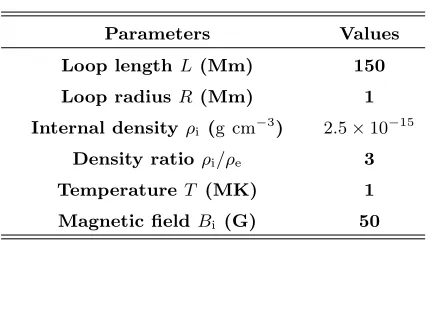
l≈0.4R, corresponding to a typical value estimated in coronal loops (Goossens et al. 2002). The initial parameters of the loop are shown in Table 1. The loop length (L= 150Mm) and radius (R= 1Mm) are chosen within the range of observations (Nakariakov et al. 1999; Aschwanden et al. 2002). The density ratio here is chosen according to the estimated value in Aschwanden et al. (2003).
We consider a uniform temperature loop (Ti =Te= 1MK), so the average temperature increase due to the mixing
between the colder tube and hotter background corona is avoided (Karampelas et al. 2017). Therefore it will be easier to identify the true wave heating effects. To maintain the magnetostatic pressure balance, the magnetic field has a slight variation from internalBi= 50G to external Be= 50.07G.
The magnetic field (50G) here is larger than previous models (e.g.,Antolin et al. 2014,2017; Karam-pelas et al. 2017) and observations (e.g.,Nakariakov & Ofman 2001;Van Doorsselaere et al. 2007,2008;
Jess et al. 2016). In this case, the energy input into the models is increased in order to obtain more noticeable heating effects.
In order to investigate the heating effects of different wave modes, we employ three models with the same initial parameters in Table 1, but different drivers on the bottom footpoint (z= 0). The first driver is a continuous, mono-periodic “dipole-like” driver, which is similar toPascoe et al.(2010) andKarampelas et al.(2017). The time-dependent velocity inside the loop (r < R) is
vi=v0 sin 2πt Pk
,0,0
, (3)
where v0 = 2km s−1 is the amplitude of the velocity. The period of the driverPk = 87s, which corresponds to the
Table 1. Parameters used in simulations
Parameters Values
Loop lengthL(Mm) 150
Loop radiusR (Mm) 1
Internal densityρi (g cm−3) 2.5×10⁻¹⁵
Density ratio ρi/ρe 3
TemperatureT (MK) 1
Magnetic field Bi (G) 50
outside the loop has the form
ve=v0R2sin 2πt
Pk
x2−y2
(x2+y2)2,
2xy
(x2+y2)2,0
. (4)
We also use a transition layer between these two regions to avoid the numerical problems, asPascoe et al.(2010) andKarampelas et al.(2017) did. The profile is similar to the density profile given by Eq. (1) and Eq. (2).
The second driver is a broad band time-dependent torsional motion, mimicking Alfv´en oscillations inside a loop. The torsional driver is inspired by the one used inBeli¨en et al.(1999). To launch this driver,vθ is described as
vθ=v0sin 2πt
PA(r) 2r R
22r
R −2
2
, r/R≤1
0, r/R >1
(5)
where v0 keeps the same value as the one of the kink driver. The period PA is a function of radial distance because
we have a non-uniform transverse density distribution. It is given byPA(r) = 2L/vA(r) = 2L p
µ0ρ(r)/B(r), varying
from its internal value of 106s to the loop boundary (r=R) value of 87s. Using these periods, we can establish Alfv´en oscillations in the uniform region (r <0.8R) and the inhomogeneous region (0.8R ≤r ≤R) with the corresponding periods on the different magnetic surfaces.
Finally, the third driver is a mixed Alfv´en and kink driver. We consider both transverse velocity (given by Eq. (3) and Eq. (4)) and torsional motions (given by Eq. (5)) simultaneously during the entire simulation. Therefore, the energy provided by the mixed driver, i.e. input energy, is at the same level as the sum of the other two drivers.
For simplicity, hereafter we name the kink driver model as “K-model”, the Alfv´en driver model as “A-model” and the mixed driver model as “M-model”. In our K-model and M-model, the drivers follow the motions of loops, making sure that the internal loop regions will always have a uniform velocity.
2.2. Numerical setup
To solve the 3-D time-dependent MHD equations, we use the PLUTO code (Mignone et al. 2007). A second-order parabolic spatial scheme is used for integration, the numerical fluxes are computed by a Roe Riemann solver. Meanwhile, a third-order Runge-Kutta algorithm is used to advance the solution to the next time level. The simulation domain is [−8,8] Mm×[−8,8] Mm×[0,150] Mm. To resolve the motions of the drivers near the footpoints, we adopt a stretched mesh with 5 cells from 0 to R and a uniform grid of 95 points fromR to L in the z-direction,. For the
x and y directions, 256 non-uniformly spaced cells are adopted, respectively. The resolution is up to 20 km in the region of|x, y| ≤2Mm. The following simulations show that this resolution is high enough to observe small structures induced by waves and instabilities.
In order to establish standing waves in loops, we fix the velocities atz=Lto be zero to mimic loops anchored in the photosphere. The other variables there are set to obey Neumann-type (zero-gradient) conditions. The z-component velocities at the bottom footpoint (z= 0) are antisymmetric andvx, vy are described by the drivers. All the lateral
3. GENERAL NUMERICAL RESULTS
We ran simulations untilt = 1500s for all three models, corresponding to roughly 14-17 periods. The maximum displacements the loops experienced are less than 1Mm, to allow us to concentrate on the subdomain of |x, y| ≤ 2Mm,0≤z≤150Mm, which is the domain with the highest resolution in thex, ydirections.
3.1. KHI eddies, resonant absorption and phase mixing
The simulation results show that the loops quickly form driven standing waves in the three models, namely standing kink (Alfv´en) waves in the K-model (A-model) and mixed (both standing kink and Alfv´en) modes in the M-model. As in previous studies, the generation of KHI can also be seen in our K-model, as is shown in Figure 1(a). The KHI develops near |y|=R, inducing the so-called TWIKH rolls (Antolin et al. 2014,2017). Figure 1(b) shows that axisymmetric vortices occur around the loop boundary in the A-model. This means that the Alfv´en oscillations in a non-uniform layer can also induce the instability, which corresponds to the prediction of Heyvaerts & Priest(1983). We can observe four clear eddies around|y|=R att= 450s in the K-model. Actually there are still four small eddies beside the clear ones around the loop boundary, which can be observed in the later instant (t= 1480s). This means that the initial unstable mode in the K-model has a wavenumber ofm= 8. In the A-model, four eddies start to occur att= 1118s, indicating that the wavenumber of the initial unstable mode ism= 4.
The results of the M-model are shown in Figure1(c). It is almost the same snapshot as in the K-model att= 450s, indicating that the torsional motions inside the loop have little influence on the instability near the loop boundary initially. When the instability induced from the torsional waves develops, the loop is deformed and the eddies extend from the boundary to almost the whole region in the M-model, as is indicated by the z-vorticity in the middle panel of Figure1. Note that the results here are attributed to not only the effect of mixed motions, but also a higher energy input in the M-model than in the other two models.
We also plot the temperature evolution of the apex in the bottom row in Figure1. The temperature increases at the locations where small eddies develop for all three models. Meanwhile, we can also observe a temperature decrease around the boundary edges. The fluctuations of the temperature probably do not mean that the heating indeed happens at thosesmall spatial-scale structures. This property is explained as adiabatic heating (cooling) rather than real dissipation (Magyar et al. 2015;Antolin et al. 2017, 2018; Karampelas et al. 2017). It should be noted that the temperature increase in the A-model is smaller than in the other two models. This means that the Alfv´en modes do not produce so many small eddies to deform the loop, therefore the density has a smaller change, leading to a smaller temperature increase.
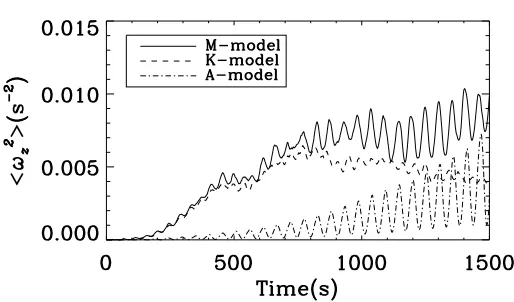
To quantify the turbulent level in our models, we examine the averaged squarez-vorticity (ω2z) at the loop apex, which is shown in Figure 2. Theω2
z in the M-model is the largest, indicating that the instability in this model is the
strongest. However, the amplitude increase of ω2
z in the A-model does not mean that more eddies are generated in
this model. It is mainly due to the increasing torsional motions at the loop apex.
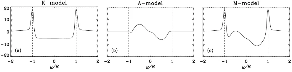
Alfv´en modes converted from kink oscillations through resonant absorption can be easily seen near the loop bound-aries (Hollweg & Yang 1988; Goossens et al. 1992,2002). Figure 3 (a)(c) shows the velocity spikes near|y| =R in the K-model and the M-model att= 255s. The spikes are the Alfv´en modes converted from kink oscillations. We do not find the Alfv´en modes at the same locations in the A-model in Figure3 (b), because no kink oscillations appear in this model. The crests near y =−0.5R and the troughs near y = 0.5R in the A-model (Figure 3 (b)) and the M-model (Figure 3(c)) are the Alfv´en oscillations coming from the drivers. It should be noted that in the M-model, the Alfv´en oscillations inside the loops can mix with the Alfv´en modes in the nonuniform layer due to their different periods, inducing the KHI. So small structures can be seen neary=−0.8R in Figure3 (c).
The Alfv´en oscillations with different frequencies can have phase mixing after a number of periods (Heyvaerts & Priest 1983). However, the scales of phase mixing eddies will decrease over time, since phase mixing will generate larger gradients and smaller scale structures. According to Mann et al.(1995) (see also Kaneko et al. 2015;Raes et al. 2017), the finest scale structures are governed by the phase mixing length
Lph=
2L t(vAe−vAi)/l
. (6)
For a very late instant t = 1480s, the phase mixing length is Lph = 0.039Mm, which is already very close to our
More eddies occur in the M-model, indicating that the mixed torsional and transverse motions deform the loop efficiently. Meanwhile, considering the small structures induced by phase mixing, we find that the mixed modes are more efficient in generating such small spatial-scale structures. Therefore, they are also likely to dissipate energy into heating more efficiently.
3.2. The saturation of oscillations
Once we set up fundamental kink oscillations in loops, the direct approach is to check the displacements or velocities at the apex, which is the location of the antinode of transverse motions. However, because of the deformation of loops, the displacement of the apex can not reveal the true oscillation properties any more. Although the deformations of our loops are not as strong asKarampelas & Van Doorsselaere(2018) due to our smaller period and larger magnetic field, to avoid the influence of the deformation, we choose the perturbations of the transverse magnetic field at the footpoint to examine the oscillation properties. For fundamental oscillations in loops, the perturbations of the transverse magnetic field will have its maximum values at the footpoints. Figure4shows the transverse perturbations of the magnetic field at the point [0.5R,0,0] in the three models. The specific point here is fixed at the bottom plane, so it is not advected following the drivers. The maximum displacement of the central loop region in this plane is about 27km, which is close to our resolution of 20km. So considering a fixed point does not significantly influence the results.
Figure 4 (a) shows the profiles of bx in the M-model and the K-model. Since the Alfv´en motions do not have x-component inside the loops, thebxhere mainly represents the kink motions. The amplitudes ofbxin the two models
are identical beforet= 1100s, showing that the kink oscillations are formed in both models and they quickly achieve a same saturation after about 3 periods due to resonant absorption. However, the Alfv´en modes need a longer time to saturate, leading to larger saturation values, as is shown in Figure4(b). The amplitudes ofbyin the M-model and
the A-model are identical before t= 800s. Then the saturation comes after that in the M-model, while it saturates after about t = 1200s in the A-model. It should be noted that the amplitude of bx in the M-model increases after
aboutt= 1200s, whereas the amplitude ofby decreases after aboutt= 1200s. This is because the point chosen here
is very close to the edge of an eddy, which makes the magnetic field vector component in the bottom plane deflect to thex-direction.
4. ENERGETICS
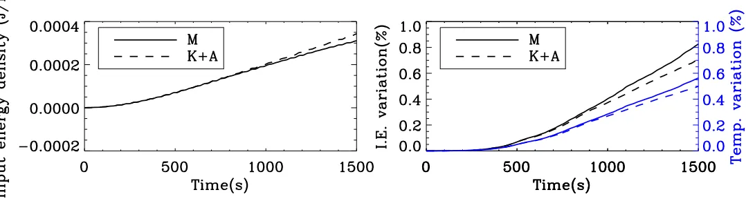
To understand the energy transfer in the systems, we study the time evolution of different kinds of energy. In the following parts, we will analyse volume averaged values in the subregion of|x| ≤2R,|y| ≤2R,0≤y≤L. The input energy, namely the Poynting flux provided by the driver, is calculated by
S(t) =−1
V
Z t
0 Z
A
S·dAdt0, (7)
following the definition in Beli¨en et al. (1999). HereS is the Poynting flux, A is the normal surface vector of the bottom planeand V is the total volume of the subregion.
Since all the variations are averaged in the same sub-volume, we will discuss energy instead of energy density in the following. In Figure5, the input energy for each model is approximately divided between the internal energy and the kinetic energy. In the K-model, a quick saturation in the kinetic energy is achieved, with a slight decrease after 10 periods. This is because the collective transverse oscillation transfers into the local turbulent motions near the loop boundary, then the TWIKH rolls break up into smaller and smaller structures. Meanwhile, considering the extension of non-uniform layer (Karampelas et al. 2017), these fine structures spread over a larger region, causing the decrease of the averaged velocity. Similar reduction in the vorticity of the K-model can also be observed in Figure2. Because of the decrease of the magnetic field perturbation in the bottom plane, the input energy experiences a slower increase in the later periods in the K-model. In the A-model and the M-model, both the kinetic energy and the magnetic energy have larger relative amplitudes, indicating later saturations. Note that in the M-model, beatings can be seen in the amplitudes of the kinetic energy and the magnetic energy due to the periods mismatch between the transverse and torsional waves.
magnetic energy in the K-model, which is also mentioned byKarampelas et al.(2017). This is due to the continuous energy input of the driver.
The input energy is almost at the same level in the K-model and the A-model, however, the internal energy increase in the A-model is much smaller than in the K-model. As is mentioned in Section 3.1, the pure torsional motions produce less eddies in the A-model. Therefore, the wave energy is less dissipated, showing a very weak heating here.
In Figure5(c), the increased input energy in the M-model becomes approximately proportional to time after about
t= 500s. We estimate the energy flux E = ∆S(t)V /∆tA∼36.5Wm−2, choosing a period from 700s to 1200s. This energy flux seems to get close to balance the radiative energy losses of quiet corona,∼100Wm−2 (Withbroe & Noyes 1977;Tomczyk et al. 2007). Furthermore, it should be noted that the input energy flux would increase for a larger input velocity. If we consider a larger amplitude driver, for example 4km s−1, the input kinetic energy would become four times larger, which would be enough to heat at least the quiet corona. Such a larger amplitude could be representative of driving velocities in e.g. the chromosphere.
To clearly compare the variations of internal energy and temperature in all three models, we examine the percentages of volume averaged values. Before that, we compare the input energy in the M-model and the sum of the other two models, as is shown in the left panel of Figure 6. They are identical before t = 1000s, then the input energy in the M-model gets smaller than the sum of the other two models. This is due to the decrease of the magnetic field perturbations near the footpoint in the M-model. The right panel of Figure 6 shows that the relative variations of internal energy and temperature monotonically increase over time. For the M-model, the relative variation of the internal energy increases to 0.83% at the end of the simulation (t= 1500s). Meanwhile, it increases to 0.71% for the sum of the other two models. Similarly, the relative variation of the temperature increases to 0.56% at the end of the simulation for the M-model, 0.49% for the sum of the other two models. Although the input energy is even smaller in the later periods of the simulation, both the internal energy and the temperature still get larger increases in the M-model. This means that the mixed modes in the M-model can indeed have enhanced heating due to a more efficient dissipation than the other two models combined. As such, the KHI rolls act as a catalyst to more efficiently dissipate the energy in other wave modes.
5. OBSERVABLE PROPERTIES
To obtain observable signals and compare to real observations, we forward modelled the numerical simulations using the FoMo code (Van Doorsselaere et al. 2016). The Fe IX 171 ˚A emission line is chosen since it is sensitive to the temperature of the models here.
broadening. Then the small structures generate rapidly around the loop boundary, showing a significant broadening. Similarly, the degraded results mimicking Hinode/EIS are shown in the bottom row of the right panel of Figure7(a). The fine structures can not be seen, only stripes are detectable.
Figure7(b) shows the forward model of the A-model. The original and degraded resolution results of the imaging models can be seen in the left panel of Figure7(b). No transverse oscillations appear, largely because the azimuthal incompressible Alfv´en modes do not disturb density. But intensity fluctuations can be seen in the original resolution results after 500s, due to the KH instability induced through phase mixing. The fluctuations are not visible in the degraded resolution. Therefore, the imaging instruments can not observe torsional Alfv´en modes at their current resolution. The middle panel of Figure 7(b) shows the Doppler velocity maps. The original resolution results (upper row) present staggered spot regions, showing that axisymmetric Alfv´en oscillations are set up in the loop. Similar to the K-model case, staggered red and blue stripes appear in the degraded models. We can also find signatures of Alfv´en oscillations in the right panel of Figure7(b), where the line width broadens inside the loop due to the torsional motions. Only stripes are detectable in the bottom row of the right panel of Figure7(b) because of the coarse resolution.
Figure7(c) shows the forward modelled results of the M-model. Fine structures can be seen in the intensity diagram as for the K-model. After about 800s, the structures seem more disordered, owing to the torsional motions of Alfv´en modes. The same degradation procedure is done to mimic the observations of SDO/AIA. Due to the limited resolution, neither the Alfv´en properties nor fine structures can be observed. This diagram is similar to the K-model case and they are both very similar to the real observations, meaning that both models could provide explanations for the decayless oscillations. The Doppler velocity map here also presents the blue and red shifts, but showing “tadpole-like” shapes. The torsional Alfv´en waves break the “bows” into smaller “tadpole” pairs. Due to the rotating and transverse motions, superpositions happen at the “heads” and cancellations happen at the regions with no “tadpole”. In the bottom row of the middle panel of Figure7(c), with the resolution of Hinode/EIS, the “tadpole-like” shapes can not be detected either, red and blue stripes are generated instead. The right column of Figure 7(c) shows the line width maps. As mentioned above, the mixed wave modes can induce more turbulent structures. Therefore, the line broadening can be observed in almost the whole loop region and disordered broadening shapes can be seen. Similar to the Doppler shift properties, the fine structures in line width can not be observed in the lower row of the right panel of Figure 7(c). Considering the frequency mismatch between the kink modes and Alfv´en modes in the M-model, we would expect a beating behaviour between these two wave modes. As is shown in Figure 7(c), the increases in Doppler velocity and line width show beatings, which can also be observed in the modulation of the kinetic and magnetic energy amplitudes in Figure5(c).
We plot the oscillation profiles of the degraded resolution intensities, as is shown in Figure8. The intensity profiles are the maximum values of Gaussian fits of the results in the left bottom of Figure7(a) and Figure7(c). The profiles of these two models do not have significant difference, indicating only kink period signals can be observed by SDO/AIA. The amplitude here is about 0.1 Mm, which agrees with the observed values inAnfinogentov et al.(2013).
We note that the staggered pattern of Doppler velocity in theA-model sets a clear difference with the case in the K-model. Actually, this has not been detected yet with EIS. It indicates that the amplitudes of torsional Alfv´en waves assumed inside the loop are probably larger than the real ones. Besides, the more localised distribution of the torsional Alfv´en modes would also influence the Doppler velocity in the coarse resolution case. The more localised the distribution is, the smaller Doppler velocity we can obtain when degrading the full numerical resolution. On top of that, if we keep the same annular velocity shape but allowing the same amplitude over a broader region that includes the boundary layer, we would have a strong superposition of Alfv´en waves with different periods, leading to very weak signals in a spectrograph. This is actually suggested in Antolin et al.
(2018) in order to explain some spicules observations. However, neither an adjustment of amplitude nor a more localised Alfv´en driver model will influence our previous statement that the KHI eddies can help to efficiently dissipate the energy in other wave modes.
6. DISCUSSIONS AND CONCLUSIONS
In this study, we simulated different oscillations in coronal loops, using a kink driver, an Alfv´en driver and a mixed Alfv´en and kink driver located at the footpoints of flux tubes. For all models, the oscillations excited in loops can lead to the KHI and generate small eddies. Especially in the M-model, the torsional motions together with transverse motions can help to generate more eddies. Besides, the Alfv´en oscillations coming from the driver inside the loop and from kink oscillations due to resonant absorption will have phase mixing, which further enhanced the instability.
We can indeed observe the increase of internal energy and temperature. The heating is enhanced for the simulation containing the mixed driver, compared with the other two models. This means that the mixed modes can lead to a more efficient energy dissipation in the turbulent state of plasma and that the KHI acts as an agent to dissipate wave energy in other modes.
According to Heyvaerts & Priest (1983), the KHI vortices can also be induced by phase mixed standing Alfv´en modes. In turn, the small vortices can also reinforce the phase mixing. This process makes more and more fine structures, which can help to dissipate wave energy more efficiently. However, in our simulations, the smaller and smaller scales will become close to the spatial numerical resolution eventually and we can not always observe the finest structures generated in loops. Generally, if we can capture smaller fine structures, the heating effects could be more pronounced.
Forward models can help to compare to the observations. Fine structures can be observed in the obtained imaging models. However, neither Alfv´en modes nor small structures are observable in the degraded resolution models. As such, the obtained imaging models agree with the decayless oscillations detected through SDO/AIA. Therefore, this study shows that Alfv´en waves can probably co-exist with transverse waves in coronal loops, leading to enhanced heating. Our spectral models reveal fine structures, the Doppler shift and the line width properties. Neither fine structures nor the particular properties can be observed in the coarse resolution models mimicking Hinode/EIS. However, beatings can be observed in Doppler velocity and line width in the mixed driver model.
We notice that in the near future, a new generation of high resolution ground based instruments, such as Daniel K. Inouye Solar Telescope (DKIST)/Diffraction Limited Near Infrared Spectropolarimeter (DL-NIRSP), will help to detect more detailed structures and reveal the energy release processes in the solar corona. The potential of this instrument has been recently predicted by Snow et al. (2018). The highest spatial sampling size of the forthcoming DKIST/DL-NIRSP is 0.0003, which is suitable for disk and limb observations, while the wide-field mode with a spatial resolution of 0.00464 will provide coronal observations. Within the temperature range in our current models (∼1MK), DL-NIRSP may have the ability to recognise the fine structures demonstrated in our forward models due to the high resolution. Similarly, forward modeling for next generation instrumentation targeting the recently proposed MUlti-slit Solar Explorer (MUSE) has been done in Antolin et al. (2017). It is shown that most of the features from the TWIKH rolls in coronal loops can be detected with a spatial resolution of 0.0033 and a spectral resolution of 25km s−1. Therefore, the future high resolution instruments may help to reveal the turbulent motions in coronal loops and distinguish different numerical models.
We assumed a uniform temperature distribution in the whole simulation domain, which can help to recognise the heating effects from waves more clearly. According to Karampelas et al. (2017), the mixing between the colder loop and the hotter corona caused a drop larger than 1.5% in the averaged temperature, while simulations with a uniform temperature lead to a rise of about 0.25%. This means that the gradient of the temperature can largely hide the expected heating from waves. Once introducing such a temperature gradient, we can hardly expect a noticeable temperature increase as in our results here, even considering the stronger plasma driving in the M-model. The larger magnetic field (50G) in our models leads to a direct consequence of a smaller transverse oscillation period (87s). However, this value is still in the scatter range of relatively shorter loop observations reported by Anfinogentov et al. (2015) and Goddard et al. (2016). Meanwhile, the kink speed in our loops is ck ≈3452km s−1, which is close to the fitting value of3300km s−1 in Goddard et al.(2016).
On top of that, the magnetic field variation with height as well as the loop curvature (Van Doorsselaere et al. 2004, 2009) are also neglected in our current models. To clarify their influence on wave heating, we will conduct a series of studies on more realistic curved loops in non-uniform force-free magnetic field in future works.
REFERENCES
Anfinogentov, S., Nistic`o, G., & Nakariakov, V. M. 2013, A&A, 560, A107
Anfinogentov, S. A., Nakariakov, V. M., & Nistic`o, G. 2015, A&A, 583, A136
Antolin, P., De Moortel, I., Van Doorsselaere, T., & Yokoyama, T. 2017, ApJ, 836, 219
Antolin, P., De Moortel, I., Van Doorsselaere, T., & Yokoyama, T. 2016, ApJL, 830, L22
Antolin, P., Schmit, D., Pereira, T. M. D., De Pontieu, B., & De Moortel, I. 2018, ApJ, 856, 44
Antolin, P., Yokoyama, T., & Van Doorsselaere, T. 2014, ApJL, 787, L22
Arregui, I., Oliver, R., & Ballester, J. L. 2012, Living Reviews in Solar Physics, 9, 2
Aschwanden, M. J. 2006, Philosophical Transactions of the Royal Society of London Series A, 364, 417
Aschwanden, M. J., de Pontieu, B., Schrijver, C. J., & Title, A. M. 2002, SoPh, 206, 99
Aschwanden, M. J., Fletcher, L., Schrijver, C. J., & Alexander, D. 1999, ApJ, 520, 880
Aschwanden, M. J., Nightingale, R. W., Andries, J., Goossens, M., & Van Doorsselaere, T. 2003, ApJ, 598, 1375
Beli¨en, A. J. C., Martens, P. C. H., & Keppens, R. 1999, ApJ, 526, 478
Cally, P. S., & Moradi, H. 2013, MNRAS, 435, 2589 Chen, Y., Feng, S. W., Li, B., et al. 2011, ApJ, 728, 147 Chen, Y., Song, H. Q., Li, B., et al. 2010, ApJ, 714, 644 De Moortel, I., & Nakariakov, V. M. 2012, Philosophical Transactions of the Royal Society of London Series A, 370, 3193
De Pontieu, B., McIntosh, S. W., Carlsson, M., et al. 2007, Science, 318, 1574
Edwin, P. M., & Roberts, B. 1983, SoPh, 88, 179 Goddard, C. R., Nistic`o, G., Nakariakov, V. M., &
Zimovets, I. V. 2016, A&A, 585, A137
Goossens, M., Andries, J., & Aschwanden, M. J. 2002, A&A, 394, L39
Goossens, M., Hollweg, J. V., & Sakurai, T. 1992, SoPh, 138, 233
Grant, S. D. T., Jess, D. B., Zaqarashvili, T. V., et al. 2018, Nature Physics, 14, 480
Guo, M.-Z., Chen, S.-X., Li, B., Xia, L.-D., & Yu, H. 2016, SoPh, 291, 877
Gupta, G. R., Banerjee, D., Teriaca, L., Imada, S., & Solanki, S. 2010, ApJ, 718, 11
He, J., Marsch, E., Tu, C., & Tian, H. 2009, ApJL, 705, L217
Heyvaerts, J., & Priest, E. R. 1983, A&A, 117, 220
Hollweg, J. V., & Yang, G. 1988, J. Geophys. Res., 93, 5423 Howson, T. A., De Moortel, I., & Antolin, P. 2017, A&A,
607, A77
Howson, T. A., De Moortel, I., & Antolin, P. 2017, A&A, 602, A74
Jess, D. B., Morton, R. J., Verth, G., et al. 2015, SSRv, 190, 103
Jess, D. B., Mathioudakis, M., Erd´elyi, R., et al. 2009, Science, 323, 1582
Jess, D. B., Reznikova, V. E., Ryans, R. S. I., et al. 2016, Nature Physics, 12, 179
Kaneko, T., Goossens, M., Soler, R., et al. 2015, ApJ, 812, 121
Karampelas, K., & Van Doorsselaere, T. 2018, A&A, 610, L9
Karampelas, K., Van Doorsselaere, T., & Antolin, P. 2017, A&A, 604, A130
Khomenko, E., & Cally, P. S. 2012, ApJ, 746, 68 Kuridze, D., Morton, R. J., Erd´elyi, R., et al. 2012, ApJ,
750, 51
Kuridze, D., Verth, G., Mathioudakis, M., et al. 2013, ApJ, 779, 82
Kwon, R.-Y., Ofman, L., Olmedo, O., et al. 2013, ApJ, 766, 55
Magyar, N., Van Doorsselaere, T., & Marcu, A. 2015, A&A, 582, A117
Mann, I. R., Wright, A. N., & Cally, P. S. 1995, J. Geophys. Res., 100, 19441
Matsumoto, T., & Shibata, K. 2010, ApJ, 710, 1857 Mignone, A., Bodo, G., Massaglia, S., et al. 2007, ApJS,
170, 228
Morton, R. J., Verth, G., Jess, D. B., et al. 2012, Nature Communications, 3, 1315
Muller, R., Roudier, T., Vigneau, J., & Auffret, H. 1994, A&A, 283, 232
Nakariakov, V. M., Anfinogentov, S. A., Nistic`o, G., & Lee, D.-H. 2016, A&A, 591, L5
Nakariakov, V. M., & Ofman, L. 2001, A&A, 372, L53 Nakariakov, V. M., Ofman, L., Deluca, E. E., Roberts, B.,
& Davila, J. M. 1999, Science, 285, 862
Nakariakov, V. M., Pilipenko, V., Heilig, B., et al. 2016, SSRv, 200, 75
Nakariakov, V. M., & Verwichte, E. 2005, Living Reviews in Solar Physics, 2, 3
Nistic`o, G., Nakariakov, V. M., & Verwichte, E. 2013, A&A, 552, A57
Ofman, L., Klimchuk, J. A., & Davila, J. M. 1998, ApJ, 493, 474
Pagano, P., Pascoe, D. J., & De Moortel, I. 2018, A&A, 616, A125
Parnell, C. E., & De Moortel, I. 2012, Philosophical Transactions of the Royal Society of London Series A, 370, 3217
Pascoe, D. J., Wright, A. N., & De Moortel, I. 2010, ApJ, 711, 990
Raes, J. O., Van Doorsselaere, T., Baes, M., & Wright, A. N. 2017, A&A, 602, A75
Ruderman, M. S., & Erd´elyi, R. 2009, SSRv, 149, 199 Schrijver, C. J., Title, A. M., Berger, T. E., et al. 1999,
SoPh, 187, 261
Snow, B., Botha, G. J. J., Scullion, E., et al. 2018, ApJ, 863, 172
Soler, R., Goossens, M., Terradas, J., & Oliver, R. 2014, ApJ, 781, 111
Soler, R., & Terradas, J. 2015, ApJ, 803, 43
Taroyan, Y., & Erd´elyi, R. 2009, SSRv, 149, 229
Terradas, J., Andries, J., Goossens, M., et al. 2008, ApJL, 687, L115
Tomczyk, S., McIntosh, S. W., Keil, S. L., et al. 2007, Science, 317, 1192
Tomczyk, S., & McIntosh, S. W. 2009, ApJ, 697, 1384 Van Doorsselaere, T., Debosscher, A., Andries, J., &
Poedts, S. 2004, A&A, 424, 1065
Van Doorsselaere, T., Nakariakov, V. M., & Verwichte, E. 2007, A&A, 473, 959
Van Doorsselaere, T., Nakariakov, V. M., Young, P. R., & Verwichte, E. 2008, A&A, 487, L17
Van Doorsselaere, T., Antolin, P., Yuan, D., Reznikova, V., & Magyar, N. 2016, Frontiers in Astronomy and Space Sciences, 3, 4
van Doorsselaere, T., Verwichte, E., & Terradas, J. 2009, SSRv, 149, 299
Verwichte, E., Nakariakov, V. M., & Cooper, F. C. 2005, A&A, 430, L65
Vranjes, J., Poedts, S., Pandey, B. P., & de Pontieu, B. 2008, A&A, 478, 553
Wentzel, D. G. 1979, A&A, 76, 20
Withbroe, G. L., & Noyes, R. W. 1977, ARA&A, 15, 363 Zajtsev, V. V., & Stepanov, A. V. 1975, Issledovaniia
(a) (b) (c)
Figure 2. Time evolution of the averaged square z-vorticity (ωz2) for the M-model (solid line), K-model (dashed line) and
Figure 3. vxprofile along they-direction atx= 0 and at the apex of the loops for the K-model (a), A-model (b) and M-model
Figure 4. Transverse magnetic field perturbations at [0.5R,0,0] in the three models. The point is a fixed one which is not advected according to the drivers. The left panel shows thebx evolution for the M-model(black line) and the K-model (blue
(a) K-model
(b) A-model
[image:19.612.50.564.79.613.2](c) M-model

![Figure 4. Transverse magnetic field perturbations at [0line). The right panel shows the.5R,0,0] in the three models](https://thumb-us.123doks.com/thumbv2/123dok_us/8733297.386869/16.612.55.557.63.210/figure-transverse-magnetic-eld-perturbations-right-panel-models.webp)