Silke Weinfurtner1, Gemma De las Cuevas2,3,4, Miguel Angel Martin-Delgado5 and Hans J. Briegel3,4 1SISSA, Via Bonomea 265, 34136, Trieste, Italy and INFN, Sezione di Trieste
2
Max-Planck-Institut f¨ur Quantenoptik, Hans-Kopfermann-Str. 1, D-85748, Garching, Germany 3
Institut f¨ur Theoretische Physik, Universit¨at Innsbruck, Technikerstraße 25, A-6020 Innsbruck, Austria 4Institut f¨ur Quantenoptik und Quanteninformation der ¨Osterreichischen
Akademie der Wissenschaften, A-6020 Innsbruck, Austria 5
Departamento de F´ısica Te´orica I, Universidad Complutense, 28040 Madrid, Spain
We present a new description of discrete space-time in 1+1 dimensions in terms of a set of elementary geometrical units that represent its independent classical degrees of freedom. This is achieved by means of a binary encoding that is ergodic in the class of space-time manifolds respecting coordinate invariance of general relativity. Space-time fluctuations can be represented in a classical lattice gas model whose Boltzmann weights are constructed with the discretized form of the Einstein-Hilbert action. Within this framework, it is possible to compute basic quantities such as the Ricci curvature tensor and the Einstein equations, and to evaluate the path integral of discrete gravity. The description as a lattice gas model also provides a novel way of quantization and, at the same time, to quantum simulation of fluctuating space-time.
PACS numbers: 04.60.-m, 45, 89.70.-a, 31.15.xk
A central task in defining a discrete version of space-time is to identify the relevant degrees of freedom. Addi-tionally, any theory of discrete spacetime must take into account coordinate invariance, which is a fundamental property of General Relativity (GR). This renders the identification of fundamental degrees of freedom non-trivial. Solving this problem corresponds to fixing the gauge of the coordinate invariance symmetry of GR at the discrete level.
Here we address this question and present a binary description of space-time in 1+1 dimensions. To do so, we borrow the discretization method of causal dynami-cal triangulation (CDT) [1]. Following this route leads to a formulation of spacetimes in terms of a statistical mechanical model, which we identify with a lattice gas model [2]. Fluctuations of spacetime are thereby rep-resented by different states of the lattice gas, and the Boltzmann factor for this statistical model is given by the discretized action of general relativity [3].
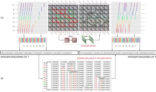
The central idea of this work is to replace the dynam-ical geometry of space-time with a fixed physdynam-ical lattice with binary degrees of freedom at its vertices. This con-struction allows us to digitalize the geometrical informa-tion content of space-times. More precisely, we show how to construct a foliated triangulation T from a bit array
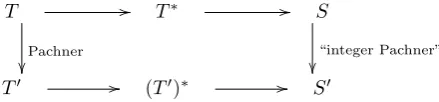
λ by using ‘forks’, and conversely how to construct a bit arrayλfrom a foliated triangulationT. For the lat-ter construction, one first mapsT to its dual T∗, T∗ to an integer string S, andS to λ, as indicated in the fol-lowing commuting diagram (the details of which will be explained below).
TriangulationT
Bit arrayλ
forks
o
o
Dual triangulationT∗ // Integer stringS
O
O
(1)
In addition, we will translate the Pachner moves to
op-erations on the integer string encoding. (The Pachner moves are transformations in the set of triangulations which are ergodic, that is, any two triangulations are re-lated by a finite sequence of Pachner moves [5]. See also [6,7] for related work.)
Finally, we will use our binary encoding to formulate meaningful quantities of discrete gravity in 1+1 dimen-sions in the natural language of information processing.
In order to establish these results, let us first recall some basic properties of CDT [1]. In CDT the continu-ous manifold of space-time is approximated by a piece-wise linear manifold [8], where the edge lengths of the simplices are assumed to be constant (space-like edges have length ledge2 and time-like edges −αl2edge, we shall henceforth assume α = −1, which is one of the points in the ‘Euclidean sector’ that gives rise to an interesting new phase [4]). Additionally, only manifolds that obey a global proper discrete time are considered, i.e.manifolds with a discrete global time foliation. On the simplicial manifold one can define curvature, an action, and other quantities [8].
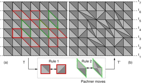
We shall here focus on the case of 1+1 dimensions, in which the configuration spaceTtis formed by all foliated triangulationsT with with t discrete proper-time steps (see Fig.1). Additionally, we restrict ourselves to sim-plicial manifolds with a fixed topology, such asS1×S1
(periodic boundary conditions (pbc) in time and space), or [0,1]×S1(open boundary conditions in time and pbc in space). We consider only connected simplicial man-ifolds; this implies, in particular, that there is at least one simplex per spatial slice. The topology of the simpli-cial manifold is characterized by the Euler characteristic
χ:=N0−N1+N2, where N0, N1, N2 is the number of vertices, edges and faces ofT, respectively. Note that in 2 dimensionsχis related to the curvature via the Gauss– Bonnet theorem.
op-erations (called Rule 1 and Rule 2; see Fig. 1). The curvatureRi is evaluated at every vertexi:
Ri=π
6−ci ci
(2)
whereci is the coordination number (i.e. number of
ad-jacent vertices) of i. The discretized Einstein–Hilbert action takes the form
S(T) =γχ−κN2, (3)
whereγandκare coupling constants related to Newton’s constant GN and the effective cosmological constant Λ
in the continuum, respectively [1]. The quantization is carried out by means of a path integral formulation of the action (3), which (for a specific topology such as [0,1]× S1) takes the form
Z= X
T∈Tt([0,1]×S1) 1
C(T)e
−S(T). (4)
HereC(T) is the order of the automorphism group ofT, and is the remnant of coordinate invariance of GR in the discrete theory.
Considerable progress has been made over the last few years —in terms of analytic in 1 + 1 [9] and numerical studies in 2 + 1 [10] and 3 + 1 [4] dimensions— to inves-tigate the continuum limit of CDT. Interesting connec-tions with other continuum quantum gravity approaches have also been established [11–13]. A connection between foliated triangulations in terms of random walks was es-tablished in [14]. Finally, let us mention that other dis-crete models of quantum gravity have been proposed, e.g. [15,16]. Although we have motivated above that we may interpret our discretizations of space-time as real at a fundamental level, we also mention that some inves-tigations have found that discrete models of spacetime tend to suffer from non-adiabaticities of the evolution of fields that live on the spacetime, which can lead to more particle production than what seems to be allowed by cosmological observational constraints [17].
I. FROM BIT ARRAYS TO TRIANGULATIONS.
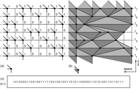
We now show how a bit array λ encodes a foliated triangulation T, as indicated in Diagram (1). The key observation is that every foliated triangulationT is built entirely (except for the boundaries) out of certain build-ing blocks that we call ’forks’. The idea is the followbuild-ing: while, obviously, the building block of a general lation is the triangle, the basic unit of a foliated triangu-lation is a pair of triangles that share a space-like edge. We identify the fork with this unit; more precisely, each fork consists of 1 ‘center’, 3 legs and 2 faces (see little diagram on bottom of Fig.2(b)). Thus, we can describe a foliated triangulation by ‘comparing’ it to a reference lattice and specifying what forks are present and what
6
t
7
t
t
3 4 5
t t t t
2
1
Rule 1 Rule 2
Pachner moves T
(a) T’ (b)
FIG. 1: CDT considers only triangulations that obey a global time foliation. (a) A foliated triangulation corresponding to a flat geometry, since the coordination number of every vertex is 6, excluding the boundaries (see Eq. (2)). Any other foli-ated triangulation, such as (b), can be obtained by applying a sequence of the Pachner moves Rule 1 and Rule 2.
forks are absent. This renders a description which is in spirit similar to that of a lattice gas model, where the description of a fluid, with molecules absent or present, is mapped to the description of a magnet with two-level spins on a fixed lattice [2].
Let us be more precise. Consider a 2D square lattice where a binary variableλnmis associated with every
ver-tex (n, m) of the lattice, with 1≤n≤Nand 1≤m≤M
(see Fig.2(a)). This forms a bit arrayλ. To transform this bit array to a foliated triangulation, we put a fork on every site (n, m) itλnm= 1, and no fork if λnm = 0.
This collection of forks defines a graphT = (V, E) in a natural way: each center of a fork defines a vertexv∈V, and its legs become edgese∈EofT. The space-like edge and the time-like edge pointing upwards connect to the first vertex to the left, and the time-like edge pointing downwards connects to the first vertex directly below or to the left (see Fig. 2). This can be formally described as follows. Letpbe a rank 3 tensor with components
pn,m,m0 :=λnm0×[(m−m0 (mod M)) + 1]. (5)
Then the vertex at site (n, m) is adjacent to the vertices at sites (n+1, a), (n, b), (n−1, c) wherea,b,care defined by the inequalities
0< pn+1,m−1,a< pn+1,m−1,m0 ∀m0 ∈[M], m06=a
0< pn,m−1,b< pn,m−1,m0 ∀m0 ∈[M], m06=b
0< pn−1,m,c< pn−1,m,m0 ∀m0 ∈[M], m06=c,
(6) where [M] ={1,2, . . . , M}.
II. FROM TRIANGULATIONS TO BIT
ARRAYS.
[image:2.595.319.567.53.199.2]t
2 6 5
1
{0,1}
3
t
7
t t t t t
4
1 1 1 1 1 0 0 1 0 0 1 1 0 0 0 0 0 1
0
0 0 1 1 1 0
0 0 0 1 0 0
0 1 1
1 1 1 0 0 1 0 0
0 1 0 1 1 0 0 1
1 1 0 0 0 0 0 1
1 0
1
0 1 0 1 1
1 1 1 0 1 1 0 1
1 0010010011010110000011010100110110111
(c)
(a) (b)
time
space
FIG. 2: From bit arrays to triangulations. The bit array (a) represents the foliated triangulation (b). Each bit stands for the presence / absence of a fork, which consists of one ver-tex, one space-like edge and two time-like edges. While the bits are fixed on a two-dimensional grid, their configuration determine the geometry, similar to a lattice gas model. (For illustration issues we have chosen non-periodic boundary con-ditions in both time and space.) To store the triangulation (b) on a double precision floating-point format (64-bit) machine a single data unit is required (c).
building block is the d-fork (short for dual fork). This consists of one time-like edge and two space-like edges “pointing to the right” (see Fig. 4(a,b)). Second, note that every d-fork crosses one space-like edge of T. We use this fact to attach the label Si ∈ {1,2, . . . , N} to
a fork i if it crosses a space-like edge at time tSi (see Fig. 4(c), where the labels are also represented as col-ors). Third, record the labels of the d-forks that appear inT∗ from left to right and write them down in an inte-ger stringS := (S1, S2, . . . , SF) (cf. Diagram (1)). This
string representation has certain symmetries. Two inte-ger strings correspond to the same dual triangulation if they are related by a sequence of the following operations:
(i) commutations of contiguous integers if the inte-gers differ by at least two, i.e. (. . . , Si, Si+1, . . .)∼
(. . . , Si+1, Si, . . .) if|Si−Si+1| ≥2;
(ii) cyclic permutations, i.e. (S1, S2, . . . , SF) ∼
(SF, S1, S2, . . . , SF−1);
(iii) inversion operation, i.e. (S1, S2, . . . , SF) ∼
(SF, SF−1, . . . , S1).
Notice that (ii) and (iii) are only applicable for periodic boundary conditions on the spatial slices, while (i) is a degeneracy introduced by the integer string encoding.
Fourth, define a string Sflat := (SN, SN, . . . , SN), consisting of complete integer-sequences, SN :=
(1,2, . . . , N). Apply operation (i) to arrange any S in
successive integer-sequences, by allowing for incomplete sequences, e.g. (1,3,4,6) (see Fig.4(d)). Fifth, define the extended stringSE by adding zeros toS wherever there is a missing element, e.g. (1,0,3,0,0,6) (see Fig. 4(e)).
Generally,
SE:= (0. . .0 | {z } Γ1
, S1,0. . .0 | {z }
Γ2
, S2, . . . , SF,0. . .0
| {z } ΓF+1
) (7)
whereA:= (N, S1, S2, . . . , SF,1), and Γ is a vector with
components Γi :=Ai+1−Ai+N−1 (modN), fori∈
{1,2, . . . , F+ 1}.
Sixth, map SE toλby arranging the entries of S in a two dimensional array of sizeN×M (going from bottom to top and left to right), and then replacing each positive entry by a 1. Formally,
λij= Θ(Sj NE −i+1) for
1≤i≤N
1≤j≤FE N
, (8)
where Θ(x) = 0 if x= 0 and Θ(x) = 1 for x > 0 (see Fig.4(f)).
A. Lattice size in binary encoding
The minimum lattice size necessary to encode all trian-gulationsT up toF forks distributed onN spatial slices is given byN×M˜, where ˜M =F−N+1. To show this, let us temporarily put aside the requirement that there is at least one fork on every spatial slice, equivalent to the re-quirement thatS contains every element in{1,2, . . . , N}
at least once. It is easy to see thatS ={X, X, . . . , X}, where all elementsX ∈ {1,2, . . . , N}are the same, max-imizes Γ = (N −X, N −1, N −1, . . . , N −1, X−1), where Γ is a vector of length F + 1, such that FE =
F + (N −1)F = F N and ˜M = F. Consequently, by reintroducing the constraint to have at least one fork per spatial slice, the stringS that will result in the largest
˜
M, has as many elements of the same kind, that are
F−N+ 1 d-forks on a single spatial sliceX. It is best to study this case using the dual brick picture, where it is straightforward to see that d-forks,X±n, forn≥1, can be moved freely in both directions by using operations (i)-(iii) (see Fig.3). Therefore any of theN−1 d-forks can be absorbed in a sequence that contains already one
X, and thus the number of sequences necessary to en-codeall possible triangulations withF forks distributed onN spatial slices isF−N+ 1. According to the map-ping, see Eq. (7) in the main text, every sequence inSE
corresponds to one row in the correspondingλ.
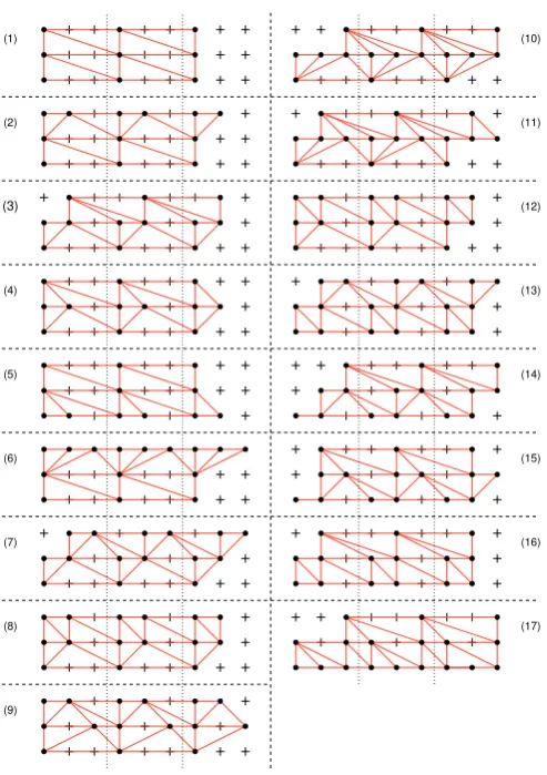
Note that by construction the integer encoding repre-sents a coordinate-free encoding of triangulations. Con-sequently, operations (i)-(iii) introduce an equivalence class on the space of all integer strings, and there exists a straightforward algorithm to single out its representa-tives. This can be illustrated with the help of a simple example, evaluating all unique histories for triangulations with 3 spatial slices from 3 to 5 forks.
[image:3.595.62.298.52.203.2](d) (c)
[image:4.595.57.297.50.128.2](b) (a)
FIG. 3: Four different dual triangulating are represented (a-d). It is shown, that by successive application of operations (i)-(iii) of the main article acting on (a) one obtains (d). The the d-forks colored in red are moved with respect to the pre-vious dual triangulations.
(1,2,2,3,3), (1,2,3,2,3), (1,2,3,3,2), (1,2,2,2,3), (1,2,2,3,2), (1,2,3,2,3), (1,1,2,3,3), (1,1,2,2,3), (1,1,2,3,2), (1,2,1,2,3), and (1,1,1,2,3). See appendix
Afor a more thorough discussion.
III. APPLICATIONS OF BINARY AND
INTEGER ENCODING.
We now rephrase various quantities of CDT in bi-nary / integer language. Last but not least, we compare the degeneracies in the configuration space in the binary with the integer encoding.
A. Binary equivalent of Ricci scalar
Consider first the Ricci scalar (Eq. (2)). The coordi-nation number of a vertex at site (n, m) is 3 (because each fork has 3 edges) plus additional ∆nm edges which
depend on the surrounding bit array; explicitly:
∆nm= F(d−m)
X
j=1
[λn+1,F(m+j−1)
+ λn+1,F(m+j)+λn+1,F(m+j)] (9)
where F(m0) := m0 (modM), anddis the index of the first non-zero entry to the left ofmgiven by 0< p(n, m+
1, d)< p(n, m+ 1, m0)∀m0 6=d (see Eqs. (5), (6)). The
Ricci scalarRnm is then given by
Rnm=π λnm
3−∆nm
3 + ∆nm
. (10)
The action (Eq. (3)) is also easily computed in the binary encoding. To compute the Euler characteristic, note that every fork is associated to one vertex, 3 edges and 2 faces, hence it does not contribute to the value of χ. Thus only forks relative to the boundary (that is, those which are placed at the boundary, either in the space or time dimension) contribute to χ. For instance, for a torus (topology S1×S1), χ = 0. The volume is then given by twice the number of forks,N2= 2F. This, together withC(T), which can be evaluated exactly for
1+1 dimensional triangulations [18], suffices to evaluate the discretized path integral (Eq. (4)).
Finally, the Pachner moves can also be expressed in the integer encoding. This allows us to show that the Pachner moves in 1+1 dimensions are ergodic, i.e they generate all simplicial triangulations.
B. Integer equivalent of Pachner moves
The Pachner moves are certain operations that when applied on a triangulation T generate other triangula-tionsT0. They are claimed to be ergodic, i.e. for any pair of triangulations, there always exists a sequence of Pach-ner moves that one can apply on one triangulation that yield the other. For foliated triangulations in 1+1 dimen-sions there are only two such moves (called Rule 1 and Rule 2, see Fig. 1 of the main text). Here we define the Pachner moves in the integer string description, that is, transformations on the integer strings which correspond to applying the Pachner move on the corresponding tri-angulation, as the following diagram illustrates.
T
Pachner
/
/ T∗ // S
“integer Pachner”
T0 // (T0)∗ // S0
(11) The action of Rule 1 (R1) is easily understood in the dual triangulation, where it simply exchanges the order of two neighboring consecutive d-forks. In the integer description it corresponds to the following operation
(. . . , Si, Si+1, . . .) R1
−−→(. . . , Si+1, Si, . . .). (12)
where|Si−Si+1|= 1. Rule 2 (R2) has an equally simple equivalent,
( . . . ,(n−1), n,(n+ 1). . .)−−→R2
( . . . ,(n−1), n, n,(n+ 1), . . .), (13)
duplicating a d-fork and placing it right next to it. It is thus clear that R1 and R2 connect different equiva-lence classes in the string encoding. This demonstrates the ergodicity of the Pachner moves in 1+1 dimensions: starting from the minimal string S = (1,2,3, . . . , N −
2, N−1, N), successive application of R1 and R2 generate all possible strings, and hence all possible triangulations. Fig.5 shows the action of the “integer Pachner moves” on triangulations mentioned in the main text.
C. Degeneracies of the various encodings
[image:4.595.329.549.316.367.2]0 2 3 4 0 6 7 1 0 0 0 5 0 0 0 0 0 4 5 6 7 0 0 3 0 0 0 0 0 2 0 0 0 0 0 1 2 3 4 5 0 0 0 0 0 0 5 6 7
0 0 0 4 5 6 7
1 2 3 4 5 6 7 1 0 4 5 0 2 0 1 0 3 0 0 0 0 0 2 0 0 0 0 0 1 2 3 4 0 0 0 1 0 0 4 5 6 7 0 0 3 4 0 6 7 0 2 3 4 0 6 7 1 0 0 0 5 0 0 0 0 0 4 5 6 7 0 0 0 0 0 0 3 0 2 0 0 0 0 0 1 2 3 4 5 0 0 0 0 0 0 5 6 7 0 0 0 4 5 6 7 1 2 3 4 5 6 t t t t t t 7 t
1 2 3 4 5 6 7 1 2 4 5 1 3 2 1 2 3 4 1 4 5 6 7 3 4 6 7 2 3 4 6 7 1 5 4 5 6 7 3 2 1 2 3 4 5 5 6 7 4 5 6 7
1234567124351212344567673467123454567132123455674567
1 2 3 4 5 6 7 1 2 4 3 5 1 2 1 2 3 4 4 5 6 7 6 7 3 4 6 7 1 2 3 4 5 4 5 6 7 1 3 2 1 2 3 4 5 5 6 7 4 5 6 7
0 0 0 0 0 0 0 0 0 0 0 0 0 0 0 0 0 0 0 0 0
0 0 0 0
0 0 0 0 0 0 0 0 0 0 0 0 0 0 0 0 0 0 0 0 0 0 0 0 0 0 0 0
0 0 3 4 0 6 7 1 0 0 4 5 6 7
1 2 3 4 0 0 0 0 2 0 0 0 0 0
1 0 3 0 0 0 0
1 2 0 4 5 0 0
1 2 3 4 5 6 7
1 0 1 1 1 1 1 1 1 1 1 1 1 0 0 0 1 1 0 0 0 1 1 1 1 0 0 1 0 0 0 0 0 0 0 1 1 0 1 0 1 1 1 1 1 1 0 0 0 0 0 0 0 1 1 0 1 0 1 0 0 0 0 0 0 1 0 0 0 1 0 0 0 0 1 1 1 1 0 0 0 0 0 0 1 1 0 1 1 1 1 0 1 1 0 0 1 1 0 1 1 1 0 0 1 0 3 7 2
1 4 5 6
[image:5.595.117.501.58.461.2](g) (f) (e) (d) (b) (c) (a)
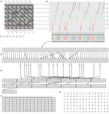
FIG. 4: From triangulations to bit arrays. The triangulationT of panel (a) (which is the same as in Fig.1(b)) is mapped to the bit array of panel (g). (a) We first construct the dual ofT (a), and redraw it to give it the appearance of a brick wall (b), where every vertical (colored) line represents a dual fork (d-fork). The dual graph is mapped to a stringS (c). Using operations (i)-(iii) we reorderS in successive incomplete integer-sequences (d), and extend the string by adding zeros where the integer-sequence is incomplete (e). Finally, we map this extended string to the bit array with Eq. (8) (f,g). (Notice that we consider here open boundary conditions on the spatial slices.)
of the configuration space. For F N we can simplify the minimum lattice size required to encode all triangula-tions toN×F. Thus the number of triangulations in the binary encoding is growing∝(2N)F, while the size of the
integer encoding grows∝NF. Since both encodings are
ergodic (in the sense of containing all triangulations with
Fforks distributed overNspatial slices at least once) the binary encoding is less efficient than the integer encoding. The integer encoding has the additional advantage that the degeneracies of the configuration space are related to algebraic symmetry operations acting on the strings (see above).
This can be demonstrated with the help of the following example. Consider the integer string
S = (1,2,3, 1,2,3, 1,2,3), representing a
triangu-lation with coordination number 6 everywhere except at the boundaries. Even for this trivial example the mapping to a binary encoding is not unique, if the lattice size is larger then 3×3. In Fig. 6 we have depicted 6 seemingly different encodings of S. Fig. 6(a-d) are simply different binary encodings ofS, while Fig.6(e-f) are mappings of S to λ after having applied various symmetry operations onS.
( 1 t t t t t t t 2 3 4 5 6 7
INTEGER ENCODING OF T
1234567 1234567 1234567 1234567 1234567 1234567 1234567 1234567 1234567 1234567 1234567 1234567 1234567 1234567 1234567 1234567 1234567 1234567 1234567 1234567
1234567 1234567 1234567 1234567
1234567 1234456767
34567 12 1234456767
34567 12 1 23 4456767
34567 12 1234456767
34567 12 1234456767
34567 12 1234456767
1324567 7 132 1243567456
1234567
132 12345674567
34
12 1234456767 567132123455674567 2
1 435
1234567 67 123 5
34567
12 1234456767 12344567132123455674567 34
12 1234456767 567132123455674567 2
1 435
1234567 67 123544
4 4 1234567 1234567 1234567 1234567 1234567 1234567 34567
12 1234456767 1234567 132123455674567 1234567
1234567 2 1 435
2 1 435
2 1 435
2 1 435
2 1 435
2 1 435
2 1 435
2 1 435
1234567 1234567 1234567 1234567 1234567 1234567
1234567 1
12345 1234 5767 1234567 123456767 12345
234567 12435 123456767 1234567 S=( ) ) ) ) ) ) ) ) ) ) ) ) ) ) 6 ( ( ( ( ( ( ( ( ( ( ( PC R1 R1 R2 R1 R1 R1 R2 R2 R1 PC PC PC S’=( (a) (b)
INTEGER ENCODING OF T’ INTEGER ANALOGUE OF PACHNER MOVES
PACHNER MOVES Rule 2 Rule 1 S’=(1,2,3,4,5,6,7,1,2,4,3,5,1,2,1,2,3,4,4,5,6,7,6,7,3,4,6,7,1,2,3,4,5,4,5,6,7,1,3,2,1,2,3,4,5,5,6,7,4,5,6,7) S=(1,2,3,4,5,6,7,1,2,3,4,5,6,7,1,2,3,4,5,6,7,1,2,3,4,5,6,7,1,2,3,4,5,6,7,1,2,3,4,5,6,7,1,2,3,4,5,6,7) 7 6 5 4 3 2
[image:6.595.53.558.50.347.2]1 1 2 3 4 5 6 7
FIG. 5: We show explicitly how to apply successively R1 and R2 on T to obtain T0 in both, the simplicial (a) and the integer string (b) encoding. In order to apply R1 it is sometimes necessary to use the pairwise commutation relations (PC), i.e. (. . . , Si, Si+1, . . .) ∼ (. . . , Si+1, Si, . . .) if |Si−Si+1| ≥ 2. Notice that the integer strings S and S0 correspond to the
triangulationsT andT0 of Fig. 1 in the main text, respectively.
(d)
(a) (b) (c)
(f) (e) 6 3 5 5 4 5 5 4 6 6 3 5 5 4 5 5 4 6 6 3 5
6 6 4
5 5 4
5 5 3 5 5 3
6 6 4
5 5 4
5 5 3
6 6 4
5 5 4
(1,2,3, 1,2,3, 1,2,3) (1,2,3, 1,2,3, 1,2,3) (1,2,3, 1,2,3, 1,2,3)
(1,2,1,3,2,3,1,2,3) −−> (1,2,3, 1,2,3, 1,2,3) (1,2,3,1,2,1,3,2,3) −−> (1,2,3, 1,2,3, 1,2,3) (1,2,3, 1,2,3, 1,2,3)
5 4 5 5 4 6
FIG. 6: Six different binary encodings of S¯ = (1,2,3, 1,2,3, 1,2,3) in a 3×4 lattice are represented. The numbers at the vertices are the coordination numbers.
IV. CONCLUSION AND OUTLOOK
We have presented a binary encoding of discrete space-time in 1+1 dimensions. To this end, we have borrowed the discretization method of CDT and shown how to compute various quantities of interest of this theory in the binary description. Our results enable us to express
a classical theory of discrete space-time as a lattice gas model. This approach has several potential applications. To begin with, it provides a natural framework for quan-tization. Forks, the elementary geometrical unit, consti-tute independent classical degrees of freedom or ’normal modes’ of discrete space-time. In the quantized theory, the presence or absence of a fork will be interpreted as elementary excitations of a quantum lattice gas. These excitations will give rise to quantum fluctuations and, more generally, to quantum states representing super-positions of different space-times. Despite using a time foliation, our approach to quantizing space-time is con-ceptually different from CDT quantum gravity, which is based on a path integral formulation.
Discretization of space-time was introduced as a regu-larization tool to compute the path integral of general rel-ativity. If one considers discrete space-time asreal, then forks could be seen as fundamental constituents of space-time, namely as basic geometric structures that connect events. A quantum formulation of this theory would nat-urally introduce quantum correlations in space-time.
[image:6.595.55.297.420.587.2]in particular, in higher dimensions we have additional geometrical constraints besides the Euler characteristic and we also have additional Pachner moves. Therefore, this important line of research calls for more elaboration and future work.
Finally, from an experimental perspective, by imple-menting quantum lattice gas models in the way we have introduced them, one could realize quantum simulations of fluctuating space-time. Such quantum simulators, ana-log or digital, could be used to simulate models of quan-tum gravity in modern quanquan-tum optics laboratories, e.g. using ultra-cold atoms in optical lattices or ion-traps [19].
Acknowledgments
We acknowledge support by the Spanish MICINN grant FIS2009-10061, the CAM research consortium QUITEMADS 2009-ESP-1594, the European Commis-sion PICC: FP7 2007-2013, Grant No. 249958, the UCM-BS grant GICC-910758, and the Austrian Science Fund (FWF) through project F04012. SW was supported by Marie Curie Actions – Career Integration Grant (CIG); Project acronym: MULTI-QG-2011 and the FQXi Mini-grant “Physics without borders”. SW would like to thank Matt Visser, Piyush Jain, and Thomas Sotiriou for en-lightening comments and discussions. GDLC acknowl-edges support from the Alexander von Humboldt foun-dation.
Appendix A: Representatives of equivalence classes in all three encodings
To evaluate the path integral of CDT in any dimen-sions analytically, one has to first single out triangu-lations which are representatives of their equivalence classes. We demonstrate how this procedure can be done in integer string encoding. First, note that to encode all triangulations of sizeV = 2F distributed overN spatial slices, one has to generate all strings containing at least
N forks and at mostF of them containing each element
of{1. . . N} at least once. We then apply symmetry
op-erations (i)-(iii) as illustrated in the following example. Consider all triangulations containing up to 5 forks
distributed over 3 spatial slices. We require at least one fork on every spatial slice; the smallest (in terms of 2-volume) triangulations contain 3 forks. The procedure to find the representatives for the equivalent classes is the following:
1. generate all possible integer strings of lengths 3, 4 and 5, with elements inSi∈ {1,2,3};
2. consider only strings that contain every element
{1,2,3} at least once (so that only connected tri-angulations are taken into account);
3. apply symmetry operations to single out unique tri-angulations / integer strings: if two integer strings are related by a sequence of the symmetry opera-tions (i–ii) they are in the same equivalence class. One representative of each equivalence class give all unique histories / triangulations. It is best to demonstrate this at hand of an example. What are the representatives of triangulations containing 4 forks distributed over 3 spatial slices? From basic combinatorics we are left with nine valid integer string encodings: S1 = (1,2,3,3), S2 = (1,3,2,3),
S3 = (1,3,3,2), S4 = (1,2,2,3), S5 = (1,2,3,2),
S6 = (1,3,2,2), S7 = (1,1,2,3), S8 = (1,1,3,2),
and S9 = (1,2,1,3). Let us to begin with fo-cus on the dual triangulations with one extra d-fork on the third row, i.e. S1, S2 and S3. Uti-lizing the symmetry operations we can show that
S2 = (1,3,2,3) = (3,1,2,3) = (1,2,3,3) = S1, and S3 = (1,3,3,2) = (3,1,3,2) = (3,3,1,2) = (3,1,2,3) = (1,2,3,3) = S1, and consequentlyS2 and S3 are redundant, and S1 is a representative. Similarly we get S6 = (1,3,2,2) = (3,1,2,2) = (1,2,2,3) = S4, S8 = (1,1,3,2) = (1,3,1,2) = (3,1,1,2) = (1,1,2,3) =S7, andS9= (1,2,3,1) = (1,1,2,3) = S7. Altogether we can for example single out the following representatives: S1,S4,S5, andS7.
Next we present the binary and the integer description for this set of triangulations explicitly. For the binary description we need to consider arrays of size N×F˜ − N+ 1 = 3×3 (see sectionIIin the main text ).
1. Representatives for 3 forks distributed over 3 spatial slices
There is only one way to distribute 3 forks on 3 spatial slices, such that
˜
S1= (1,2,3) → S˜1E= (1,2,3, 0,0,0, 0,0,0) → λ( ˜S1E) =
1 0 0 1 0 0 1 0 0
(17) (5)
(9)
(1) (10)
(11)
(4) (2)
(12)
(13)
(8) (3)
(14)
(16) (7)
[image:8.595.54.301.61.411.2](15) (6)
FIG. 7: The representatives of the equivalence classes for all triangulations up to 5 forks distributed on 3 spatial slices are shown. Notice that because of the periodic boundary conditions on the spatial slices, it is advantageous to display three periods (indicated by the dotted vertical lines).
2. Representatives for 4 forks distributed over 3 spatial slices
After applying the symmetry operations we are left with four representatives:
˜
S2= (1,2,3,3) → S˜2E= (1,2,3, 0,0,3, 0,0,0) → λ( ˜S
E 2) =
1 1 0 1 0 0 1 0 0
, see FIG.7(2); (A2)
˜
S3= (1,2,2,3) → S˜3E= (1,2,0, 0,2,3, 0,0,0) → λ( ˜S3E) =
0 1 0 1 1 0 1 0 0
, see FIG.7(3); (A3)
˜
S4= (1,2,3,2) → S˜4E= (1,2,3, 0,2,0, 0,0,0) → λ( ˜S4E) =
1 0 0 1 1 0 1 0 0
, see FIG.7(4) (A4)
˜
S5= (1,1,2,3) → S˜5E= (1,2,3, 1,0,0, 0,0,0) → λ( ˜S
E 5) =
1 0 0 1 0 0 1 1 0
3. Representatives for 5 forks distributed over 3 spatial slices
After applying the symmetry operations we are left with 12 representatives:
˜
S6= (1,2,3,3,3) → S˜6E= (1,2,3, 0,0,3, 0,0,3) → λ( ˜SE2) =
1 1 1 1 0 0 1 0 0
, see FIG.7(6); (A6)
˜
S7= (1,2,2,3,3) → S˜7E= (1,2,0, 0,2,3, 0,0,3) → λ( ˜SE7) =
0 1 1 1 1 0 1 0 0
, see FIG.7(7); (A7)
˜
S8= (1,2,3,2,3) → S˜8E= (1,2,3, 0,2,3, 0,0,0) → λ( ˜SE8) =
1 1 0 1 1 0 1 0 0
, see FIG.7(8); (A8)
˜
S9= (1,2,3,3,2) → S˜9E= (1,2,3, 0,0,3, 0,2,0) → λ( ˜SE9) =
1 1 0 1 0 1 1 0 0
, see FIG.7(9); (A9)
˜
S10= (1,2,2,2,3) → S˜10E = (1,2,0, 0,2,0, 0,2,3) → λ( ˜S
E 10) =
0 0 1 1 1 1 1 0 0
, see FIG.7(10); (A10)
˜
S11= (1,2,2,3,2) → S˜11E = (1,2,0, 0,2,3, 0,2,0) → λ( ˜S2E) =
0 1 0 1 1 1 1 0 0
, see FIG.7(11); (A11)
˜
S12= (1,2,3,2,3) → S˜12E = (1,2,3, 0,2,3, 0,0,0) → λ( ˜S12E) =
1 1 0 1 1 0 1 0 0
, see FIG.7(12); (A12)
˜
S13= (1,1,2,3,3) → S˜13E = (1,0,0, 1,2,3, 0,0,3) → λ( ˜S13E) =
0 1 1 0 1 0 1 1 0
, see FIG.7(13); (A13)
˜
S14= (1,1,2,2,3) → S˜14E = (1,0,0, 1,2,0, 0,2,3) → λ( ˜S14E) =
0 0 1 0 1 1 1 1 0
, see FIG.7(14); (A14)
˜
S15= (1,1,2,3,2) → S˜15E = (1,0,0, 1,2,3, 0,2,0) → λ( ˜S15E) =
0 1 0 0 1 1 1 1 0
, see FIG.7(15); (A15)
˜
S16= (1,2,1,2,3) → S˜16E = (1,2,0, 1,2,3, 0,0,0) → λ( ˜S16E) =
0 1 0 1 1 0 1 1 0
, see FIG.7(16); (A16)
˜
S17= (1,1,1,2,3) → S˜17E = (1,0,0, 1,0,0, 1,2,3) → λ( ˜S17E) =
0 0 1 0 0 1 1 1 1
, see FIG.7(17); (A17)
[1] J. Ambjørn, J. Jurkiewicz, and R. Loll, Phys. Rev. Lett. 85, 924 (2000);ibid., Phys. Rev. D64044011 (2001).
crit-ical phenomena, Oxford University Press (1987). [3] T. Regge, General relativity without coordinates,Nuovo
Cim., 19:558–571, 1961.
[4] J. Ambjørn, J. Jurkiewicz, and R. Loll, Phys. Rev. Lett. 93,131301 (2004).
[5] U. Pachner, European Journal of Combinatorics,12, 129 (1991).
[6] A. Kempf, Phys. Rev. Lett. 103, 231301 (2009). [7] A. Kempf, arxiv:1302.3680 (2013).
[8] F. David, Simplicial quantum gravity and random lat-tices (Elsevier, Amsterdam, 1995), Session LVII, p. 679;
ibid. Nucl. Phys. B 257, 45 (1985); V. Kazakov, Phys. Lett. B150, 282 (1985).
[9] J. Ambjørn and R. Loll. Nucl. Phys. B536, 407 (1998). [10] D. Benedetti, R. Loll, and F. Zamponi, Phys. Rev. D76,
104022 (2007).
[11] P. Hoˇrava, Phys. Rev. Lett.102, 161301 (2009).
[12] T. P. Sotiriou, M. Visser, and S. Weinfurtner, Phys. Rev. Lett.107, 131303 (2011).
[13] M. Reuter and F. Saueressig, JHEP1112, 012 (2011). [14] P. Di Francesco, E. Guitter, C. Kristjansen, Nucl. Phys.
B567, 515 (2000).
[15] L. Bombelli, J. Lee, D. Meyer and R. Sorkin, Phys. Rev. Lett.59, 521 (1987).
[16] T. Konopka, F. Markopolou and S. Severini, Phys. Rev. D77, 104029 (2008).
[17] B. Z. Foster, Th. Jacobson, JHEP 0408 (2004) 024 [18] B. Dittrich and R. Loll, Class. Quantum Grav.23, 3849
(2006).