Proceedings of the 57th Annual Meeting of the Association for Computational Linguistics, pages 3025–3036 3025
STACL: Simultaneous Translation with Implicit Anticipation and
Controllable Latency using Prefix-to-Prefix Framework
∗Mingbo Ma1,3 Liang Huang1,3 Hao Xiong2 Renjie Zheng3 Kaibo Liu1,3 Baigong Zheng1 Chuanqiang Zhang2 Zhongjun He2 Hairong Liu1 Xing Li1 Hua Wu2 Haifeng Wang2
1Baidu Research, Sunnyvale, CA, USA
2Baidu, Inc., Beijing, China
3Oregon State University, Corvallis, OR, USA
{mingboma, lianghuang, xionghao05, hezhongjun}@baidu.com
Abstract
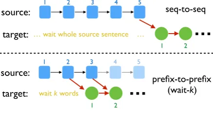
Simultaneous translation, which translates sentences before they are finished, is use-ful in many scenarios but is notoriously dif-ficult due to word-order differences. While the conventional seq-to-seq framework is only suitable for full-sentence translation, we pro-pose a novel prefix-to-prefix framework for si-multaneous translation that implicitly learns to anticipate in a single translation model. Within this framework, we present a very sim-ple yet surprisingly effective “wait-k” policy
trainedto generate the target sentence
concur-rently with the source sentence, but alwaysk
words behind. Experiments show our strat-egy achieves low latency and reasonable qual-ity (compared to full-sentence translation) on
4 directions: zh↔en and de↔en.
1 Introduction
Simultaneous translation aims to automate simul-taneous interpretation, which translates concur-rently with the source-language speech, with a de-lay of only a few seconds. Thisadditivelatency is much more desirable than themultiplicative2× slowdown in consecutive interpretation.
With this appealing property, simultaneous in-terpretation has been widely used in many scenar-ios including multilateral organizations (UN/EU), and international summits (APEC/G-20). How-ever, due to the concurrent comprehension and production in two languages, it is extremely chal-lenging and exhausting for humans: the num-ber of qualified simultaneous interpreters world-wide is very limited, and each can only last for about 15-30 minutes in one turn, whose error rates grow exponentially after just minutes of interpret-ing (Moser-Mercer et al., 1998). Moreover,
lim-∗
M.M. and L.H. contributed equally; L.H. conceived the main ideas (prefix-to-prefix and wait-k) and directed the project, while M.M. led the implementations on RNN and Transformer. See example videos, media reports, code, and
data athttps://simultrans-demo.github.io/.
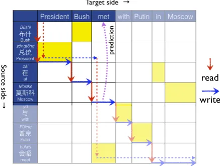
President Bush met with Putin in Moscow
Bùshí Bush zǒngtǒng President zài at Mòsīkē
Moscow yǔ
with Pǔjīng
Putin huìwù meet
pr
ed
icti
on
read
write
So
ur
ce
sid
e
→
[image:1.595.308.527.220.385.2]Target side →
Figure 1: Our wait-kmodel emits target wordytgiven
source-side prefix x1... xt+k−1, often before seeing
the corresponding source word (here k=2, outputing
y3=“met” beforex7=“hu`ıw`u”). Without anticipation, a
5-word wait is needed (dashed arrows). See also Fig.2.
ited memory forces human interpreters to rou-tinely omit source content (He et al.,2016). There-fore, there is a critical need to develop simultane-ous machine translation techniques to reduce the burden of human interpreters and make it more ac-cessible and affordable.
Unfortunately, simultaneous translation is also notoriously difficult for machines, due in large part to the diverging word order between the source and target languages. For example, think about simultaneously translating an SOV language such as Japanese or German to an SVO language such as English or Chinese:1 you have to wait un-til the source language verb. As a result, exist-ing so-called “real-time” translation systems resort to conventional full-sentence translation, causing an undesirable latency of at least one sentence. Some researchers, on the other hand, have noticed the importance of verbs in SOV→SVO translation
1 Technically, German is SOV+V2 in main clauses, and
B `ush´ı zˇongtˇong z`ai M`os¯ık¯e yˇu Pˇuj¯ıng hu`ıw`u 布
布
布什什什 总总总统统统 在在在 莫莫莫斯斯斯科科科与 普京 会晤
Bush president in Moscow with/and Putin meet
(a) simultaneous: our wait-2 ...wait 2 words... pres. bush met with putin in moscow
(b) non-simultaneous baseline ... wait whole sentence ... pres. bushmetwith putin in moscow
(c) simultaneous: test-time wait-2 ...wait 2 words... pres. bush in moscow and pol- ite meeting
布什 总统 在莫斯科与 普京会晤
[image:2.595.71.524.63.154.2](d) simultaneous: non-predictive ...wait 2 words... pres. bush ... wait 5 words ... metwith putin in moscow
Figure 2: Another view of Fig.1, highlighting the prediction of English“met”corresponding to the
sentence-final Chinese verbhu`ıw`u. (a) Our wait-kpolicy (herek = 2) translates concurrently with the source sentence,
but alwayskwords behind. It correclty predicts the English verb given just the first 4 Chinese words (in bold),
lit. “Bush president in Moscow”, because it is trained in a prefix-to-prefix fashion (Sec.3), and the training data
contains many prefix-pairs in the form of (Xz`aiY ..., X met ...). (c) The test-time wait-kdecoding (Sec.3.2) using
the full-sentence model in (b) can not anticipate and produces nonsense translation. (d) A simultaneous translator
without anticipation such asGu et al.(2017) has to wait 5 words.
(Grissom II et al.,2016), and have attempted to re-duce latency by explicitly predicting the sentence-final German (Grissom II et al., 2014) or English verbs (Matsubarayx et al.,2000), which is limited to this particular case, or unseen syntactic con-stituents (Oda et al.,2015;He et al.,2015), which requires incremental parsing on the source sen-tence. Some researchers propose to translate on an optimized sentence segment level to get bet-ter translation accuracy (Oda et al., 2014; Fujita et al., 2013; Bangalore et al., 2012). More re-cently,Gu et al.(2017) propose a two-stage model whose base model is a full-sentence model, On top of that, they use a READ/WRITE (R/W) model to decide, at every step, whether to wait for an-other source word (READ) or to emit a target word using the pretrained base model (WRITE), and this R/W model is trained by reinforcement learn-ing to prefer (rather than enforce) a specific la-tency, without updating the base model. All these efforts have the following major limitations: (a) none of them can achieve any arbitrary given la-tency such as “3-word delay”; (b) their base trans-lation model is still trained on full sentences; and (c) their systems are complicated, involving many components (such as pretrained model, prediction, and RL) and are difficult to train.
We instead present a very simple yet effective solution, designing a novel prefix-to-prefix frame-work that predicts target words using only pre-fixes of the source sentence. Within this frame-work, we study a special case, the “wait-k” policy, whose translation is alwayskwords behind the in-put. Consider the Chinese-to-English example in Figs. 1–2, where the translation of the sentence-final Chinese verb hu`ıw`u (“meet”) needs to be
emitted earlier to avoid a long delay. Our wait-2 model correctly anticipates the English verb given only the first 4 Chinese words (which provide enough clue for this prediction given many sim-ilar prefixes in the training data). We make the following contributions:
• Our prefix-to-prefix framework is tailored to simultaneous translation and trained from scratch without using full-sentence models.
• It seamlessly integrates implicit anticipation and translation in a single model that directly predictstargetwords without explictly hallu-cinatingsourceones.
• As a special case, we present a “wait-k” pol-icy that can satisfy any latency requirements.
• This strategy can be applied to most sequence-to-sequence models with relatively minor changes. Due to space constraints, we only present its performance the Trans-former (Vaswani et al.,2017), though our ini-tial experiments on RNNs (Bahdanau et al.,
2014) showed equally strong results (see our November 2018 arXiv version https: //arxiv.org/abs/1810.08398v3).
• Experiments show our strategy achieves low latency and reasonable BLEU scores (com-pared to full-sentence translation baselines) on 4 directions: zh↔en and de↔en.
2 Preliminaries: Full-Sentence NMT
We first briefly review standard (full-sentence) neural translation to set up the notations.
…
… wait whole source sentence …1 2
source:
target:
4
1 2 3 5
seq-to-seq
4
1 2 3
…
wait k words1 2
source:
target:
5
[image:3.595.74.293.64.180.2]prefix-to-prefix (wait-k)
Figure 3: Seq-to-seq vs. our prefix-to-prefix frame-works (showing wait-2 as an example).
the input sequence x = (x1, ..., xn) where each
xi ∈Rdx is a word embedding ofdx dimensions,
and produces a new sequence of hidden states
h = f(x) = (h1, ..., hn). The encoding function
f can be implemented by RNN or Transformer. On the other hand, a (greedy) decoder predicts the next output wordytgiven the source sequence
(actually its representationh) and previously gen-erated words, denotedy<t = (y1, ..., yt−1). The
decoder stops when it emits<eos>, and the final
hy-pothesisy= (y1, ...,<eos>)has probability
p(y|x) =Q|y|
t=1p(yt|x,y<t) (1)
At training time, we maximize the conditional probability of each ground-truth target sentencey?
given inputx over the whole training dataD, or equivalently minimizing the following loss:
`(D) =−P
(x,y?)∈Dlogp(y?|x) (2)
3 Prefix-to-Prefix and Wait-k Policy
In full-sentence translation (Sec.2), eachyiis
pre-dicted using the entire source sentencex. But in simultaneous translation, we need to translate con-currently with the (growing) source sentence, so we design a new prefix-to-prefix architecture to (be trained to) predict using a source prefix.
3.1 Prefix-to-Prefix Architecture
Definition 1. Let g(t) be a monotonic
non-decreasingfunction oftthat denotes the number
of source words processed by the encoder when deciding the target wordyt.
For example, in Figs.1–2, g(3) = 4, i.e., a 4-word Chinese prefix is used to predicty3=“met”.
We use the source prefix(x1, ..., xg(t))rather than
the whole x to predict yt: p(yt | x≤g(t),y<t).
Therefore the decoding probability is:
pg(y|x) =Q
|y|
t=1p(yt|x≤g(t),y<t) (3)
and given trainingD, the training objective is:
`g(D) =−P(x,y?)∈Dlogpg(y? |x) (4)
Generally speaking, g(t)can be used to repre-sent any arbitrary policy, and we give two special cases whereg(t)is constant: (a)g(t) =|x|: base-line full-sentence translation; (b)g(t) = 0: an “or-acle” that does not rely on any source information. Note that in any case,0≤g(t)≤ |x|for allt.
Definition 2. We define the “cut-off” step,
τg(|x|), to be the decoding step when source
sen-tence finishes:
τg(|x|) = min{t|g(t) =|x|} (5)
For example, in Figs.1–2, the cut-off step is 6, i.e., the Chinese sentence finishes right beforey6=“in”.
Training vs. Test-Time Prefix-to-Prefix. While
most previous work in simultaneous translation, in particularBangalore et al.(2012) andGu et al.
(2017), might be seen as special cases in this framework, we note that only theirdecoders are prefix-to-prefix, while their training is still sentence-based. In other words, they use a full-sentence translation model to do simultaneous de-coding, which is a mismatch between training and testing. The essence of our idea, however, is to train the model to predict using source pre-fixes. Most importantly, this new training implic-itly learns anticipation as a by-product, overcom-ing word-order differences such as SOV→SVO. Using the example in Figs. 1–2, the anticipation of the English verb is possible because the train-ing data contains many prefix-pairs in the form of (X z`aiY ..., X met ...), thus although the pre-fixx≤4=“B`ush´ı zˇongtˇong z`ai M`osik¯e” (lit. “Bush
president in Moscow”) does not contain the verb, it still provides enough clue to predict “met”.
3.2 Wait-kPolicy
using the first 3 source words, etc; see Fig.3. More formally, itsg(t)is defined as follows:
gwait-k(t) = min{k+t−1,|x|} (6)
For this policy, the cut-off pointτgwait-k(|x|)is
ex-actly|x| −k+ 1(see Fig.14). From this step on, gwait-k(t)is fixed to|x|, which means the
remain-ing target words (includremain-ing this step) are generated using the full source sentence, similar to conven-tional MT. We call this part of output,y≥|x|−k, the
“tail”, and can perform beam search on it (which we call “tail beam search”), but all earlier words are generated greedily one by one (see Appendix).
Test-Time Wait-k. As an example of
test-time prefix-to-prefix in the above subsection, we present a very simple “test-time wait-k” method, i.e., using a full-sentence model but decoding it with a wait-kpolicy (see also Fig.2(c)). Our ex-periments show that this method, without the an-ticipation capability, performs much worse than our genuine wait-kwhenkis small, but gradually catches up, and eventually both methods approach the full-sentence baseline (k=∞).
4 New Latency Metric: Average Lagging
Beside translation quality, latency is another cru-cial aspect for evaluating simultaneous translation. We first review existing latency metrics, highlight-ing their limitations, aand then propose our new latency metric that address these limitations.
4.1 Existing Metrics: CW and AP
Consecutive Wait (CW) (Gu et al., 2017) is the number of source words waited between two target words. Using our notation, for a policy g(·), the per-step CW at steptisCWg(t) =g(t)−g(t−1).
The CW of a sentence-pair (x,y) is the average CW over all consecutive wait segments:
CWg(x,y) = P|y|
t=1CWg(t) P|y|
t=11CWg(t)>0
= |x|
P|y|
t=11CWg(t)>0
In other words, CW measures the average source segment length (the best case is 1 for word-by-word translation or our wait-1 and the worst case is |x|for full-sentence MT). The drawback of CW is that CW is local latency measurement which is insensitive to the actual lagging behind.
Another latency measurement, Average Propor-tion (AP) (Cho and Esipova,2016) measures the proportion of the area above a policy path in Fig.1:
So
ur
ce
→
Target→
1 2 3 4 5 6 7 8 9 10
So
ur
ce
→
Target→
[image:4.595.309.526.65.179.2]1 2 3 4 5 6 7 8 9 10 11 12 13
Figure 4: Illustration of our proposed Average Lagging latency metric. The left figure shows a simple case
when |x| = |y| while the right figure shows a more
general case when|x| 6= |y|. The red policy is
wait-4, the yellow is wait-1, and the thick black is a policy whose AL is 0.
APg(x,y) =
1
|x| |y|
P|y|
t=1g(t) (7)
AP has two major flaws: First, it is sensitive to input length. For example, consider our wait-1 policy. When|x| = |y| = 1, AP is 1, and when |x| = |y| = 2, AP is 0.75, and eventually AP approaches 0.5 when|x| = |y| → ∞. However, in all these cases, there is a one word delay, so AP is not fair between long and short sentences. Second, being a percentage, it is not obvious to the user the actual delays in number of words.
4.2 New Metric: Average Lagging
Inspired by the idea of “lagging behind the ideal policy”, we propose a new metric called “average lagging” (AL), shown in Fig.4. The goal of AL is to quantify the degree the user is out of sync with the speaker, in terms of the number of source words. The left figure shows a special case when |x| = |y|for simplicity reasons. The thick black line indicates the “wait-0” policy where the de-coder is alway one wordaheadof the encoder and we define this policy to have an AL of 0. The diag-onal yellow policy is our “wait-1” which is always one word behind the wait-0 policy. In this case, we define its AL to be 1. The red policy is our wait-4, and it is always 4 words behind the wait-0 policy, so its AL is 4. Note that in both cases, we only count up to (but including) the cut-off point (indicated by the horizontal yellow/red arrows, or 10 and 7, resp.) because the tail can be generated instantly without further delay. More formally, for the ideal case where|x=|y|, we can define:
ALg(x,y) =
1
τg(|x|)
τg(|x|)
X
t=1
We can infer that the AL for wait-kis exactlyk. When we have more realistic cases like the right side of Fig. 4 when |x| < |y|, there are more and more delays accumulated when target sen-tence grows.For example, for the yellow wait-1 policy has a delay of more than 3 words at decod-ing its cut-off step 10, and the red wait-4 policy has a delay of almost 6 words at its cut-off step 7. This difference is mainly caused by the tgt/src ratio. For the right example, there are 1.3target words per source word. More generally, we need to offset the “wait-0” policy and redefine:
ALg(x,y) =
1
τg(|x|)
τg(|x|)
X
t=1
g(t)−t−1
r (9)
where τg(|x|) denotes the cut-off step, andr =
|y|/|x|is the target-to-source length ratio. We ob-serve that wait-kwith catchup has an AL'k.
5 Implementation Details
While RNN-based implementation of our wait-k model is straightforward and our initial experi-ments showed equally strong results, due to space constraints we will only present Transformer-based results. Here we describe the implemen-tation details for training a prefix-to-prefix Trans-former, which is a bit more involved than RNN.
5.1 Background: Full-Sentence Transformer
We first briefly review the Transformer architec-ture step by step to highlight the difference be-tween the conventional and simultaneous Trans-former. The encoder of Transformer works in a self-attention fashion and takes an input sequence
x, and produces a new sequence of hidden states
z= (z1, ..., zn)wherezi∈Rdz is as follows:
zi =Pnj=1αij PWV(xj) (10)
HerePWV(·)is a projection function from the in-put space to the value space, and αij denotes the
attention weights:
αij=
expeij
Pn
l=1expeil
, eij=
PWQ(xi)PWV(xj)
T
√ dx
(11) where eij measures similarity between inputs.
HerePWQ(xi) andPWK(xj) project xi andxj to query and key spaces, resp. We use 6 layers of self-attention and usehto denote the top layer out-put sequence (i.e., the source context).
On the decoder side, during training time, the gold output sequence y∗ = (y∗1, ..., ym∗) goes through the same self-attention to generate hid-den self-attended state sequencec = (c1, ..., cm).
Note that because decoding is incremental, we let αij = 0ifj > iin Eq.11to restrict self-attention
to previously generated words.
In each layer, after we gather all the hidden representations for each target word through self-attention, we perform target-to-source attention:
c0i =Pn
j=1βij PWV0(hj)
similar to self-attention,βij measures the
similar-ity betweenhj andcias in Eq.11.
5.2 Training Simultaneous Transformer
Simultaneous translation requires feeding the source words incrementally to the encoder, but a naive implementation of such incremental en-coder/decoder is inefficient. Below we describe a faster implementation.
For the encoder, during training time, we still feed the entire sentence at once to the encoder. But different from the self-attention layer in con-ventional Transformer (Eq.11), we constrain each source word to attend to its predecessors only (similar to decoder-side self-attention), effectively simulating an incremental encoder:
α(t)ij =
expe(ijt)
Pg(t) l=1expe
(t) il
if i, j≤g(t)
0 otherwise
e(t)ij =
(P
WQ(xi)PWK(xj)T √
dx if i, j≤g(t)
−∞ otherwise
Then we have a newly defined hidden state se-quencez(t)= (z(t)
1 , ..., z (t)
n )at decoding stept:
zi(t)=Pn
j=1α
(t)
ij PWV(xj) (12)
When a new source word is received, all previous source words need to adjust their representations.
6 Experiments
6.1 Datasets and Systems Settings
We evaluate our work on four simultaneous translation directions: German↔English and Chinese↔English. For the training data, we use the parallel corpora available from WMT152
2
2
4
6
8
10
Average Lagging (de en)
15
20
25
30
1-ref BLEU
k=1
k=1
k=3
k=3
k=5
k=5
k=7
k=7
k=9
k=9
28.6
wait-k test-time wait-k2
4
6
Consecutive Wait (de en)
15
20
25
30
1-ref BLEU
k=1
k=1
k=3
k=3
k=5
k=5
k=7
k=7
k=9
k=9
28.6
wait-k [image:6.595.90.481.68.211.2]test-time wait-k
Figure 5: Translation quality against latency metrics (AL and CW) on German-to-English simultaneous
transla-tion, showing wait-kand test-time wait-kresults, full-sentence baselines, and our adaptation ofGu et al.(2017)
(I:CW=2;H:CW=5;:CW=8), all based on the same Transformer.FI:full-sentence (greedy and beam-search).
2
4
6
8
Average Lagging (en de)
10
15
20
25
1-ref BLEU
k=1k=1
k=3
k=3
k=5
k=5
k=7
k=7
k=9
k=9
26.6
wait-k test-time wait-k2
4
Consecutive Wait (en de)
10
15
20
25
1-ref BLEU
k=1k=1
k=3
k=3
k=5
k=5
k=7
k=7
k=9
k=9
26.6
wait-k [image:6.595.98.485.261.404.2]test-time wait-k
Figure 6: Translation quality against latency metrics on English-to-German simultaneous translation.
1
3
5
7
9 11
Average Lagging (zh en)
15
20
25
30
35
40
4-ref BLEU
k=1
k=3 k=5
k=7 k=9
k=1 k=3
k=5
k=7 k=9
wait-k test-time wait-k
33.14
0
2
4
6
Consecutive Wait (zh en)
15
20
25
30
35
40
4-ref BLEU
k=1
35
7 9
k=1 3
57 9
wait-k test-time wait-k
[image:6.595.87.484.433.575.2]33.14
Figure 7: Translation quality against latency on Chinese-to-English simultaneous translation.
1
3
5
7
9
11
Average Lagging (en zh)
7.5
10.0
12.5
15.0
17.5
20.0
22.5
1-ref BLEU
k=1k=3 k=5
k=7 k=9
k=1 k=3
k=5 k=7 k=9
wait-k test-time wait-k
33.14
2
4
6
Consecutive Wait (en zh)
7.5
10.0
12.5
15.0
17.5
20.0
22.5
1-ref BLEU
k=1
35
7 9
k=1 3
57 9
wait-k test-time wait-k
33.14
[image:6.595.83.482.435.719.2]Train Test
k=1 k=3 k=5 k=7 k=9 k=∞
k0=1 34.1 33.3 31.8 31.2 30.0 15.4 k0=3 34.7 36.7 37.1 36.7 36.7 18.3 k0=5 30.7 36.7 37.8 38.4 38.6 22.4 k0=7 31.0 37.0 39.4 40.0 39.8 23.7
[image:7.595.307.525.61.167.2]k0=9 26.4 35.6 39.1 40.1 41.0 28.6 k0=∞ 21.8 30.2 36.0 38.9 39.9 43.2
Table 1: wait-kpolicy in training and test (4-ref BLEU,
zh→en dev set). The bottom row is “test-time wait-k”.
Bold: best in a column; italic: best in a row.
for German↔English (4.5M sentence pairs) and NIST corpus for Chinese↔English (2M sentence pairs). We first apply BPE (Sennrich et al.,
2015) on all texts in order to reduce the vo-cabulary sizes. For German↔English evalua-tion, we use newstest-2013 (dev) as our dev set and newstest-2015 (test) as our test set, with 3,000 and 2,169 sentence pairs, respectively. For Chinese↔English evaluation, we use NIST 2006 and NIST 2008 as our dev and test sets. They con-tain 616 and 691 Chinese sentences, each with 4 English references. When translating from Chi-nese to English, we report 4-reference BLEU scores, and in the reverse direction, we use the second among the four English references as the source text, and report 1-reference BLEU scores.
Our implementation is adapted from PyTorch-based OpenNMT (Klein et al.,2017). Our Trans-former is essentially the same as the base model from the original paper (Vaswani et al.,2017).
6.2 Quality and Latency of Wait-kModel
Tab.1 shows the results of a model trained with wait-k0 but decoded with wait-k(where∞means full-sentence). Our wait-kis the diagonal, and the last row is the “test-time wait-k” decoding. Also, the best results of wait-kdecoding is often from a model trained with a slightly largerk0.
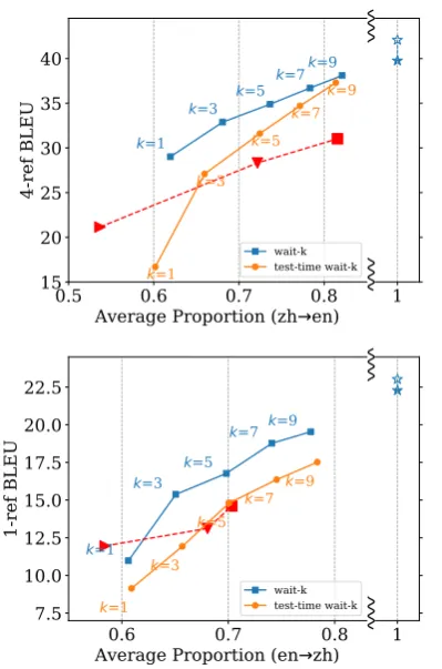
Figs. 5–8 plot translation quality (in BLEU) against latency (in AL and CW) for full-sentence baselines, our wait-k, test-time wait-k(using full-sentence models), and our adaptation ofGu et al.
(2017) from RNN to Transformer3 on the same Transformer baseline. In all these figures, we ob-serve that, ask increases, (a) wait-k improves in BLEU score and worsens in latency, and (b) the
3
However, it is worth noting that, despite our best efforts, we failed to reproduce their work on their original RNN, re-gardless of using their code or our own. That being said, our successful implementation of their work on Transformer is also a notable contribution of this work. By contrast, it is very
easy to make wait-kwork on either RNN or Transformer.
k=3 k=5 k=7 k=3 k=5 k=7
zh→en en→zh
sent-level % 33 21 9 52 27 17
word-level % 2.5 1.5 0.6 5.8 3.4 1.4
accuracy 55.4 56.3 66.7 18.6 20.9 22.2
de→en en→de
sent-level % 44 27 8 28 2 0
word-level % 4.5 1.5 0.6 1.4 0.1 0.0
[image:7.595.75.291.62.156.2]accuracy 26.0 56.0 60.0 10.7 50.0 n/a
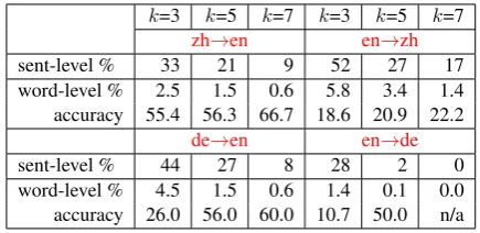
Table 2: Human evaluation for all four directions (100 examples each from dev sets). We report sentence- and word-level anticipation rates, and the word-level antic-ipation accuracy (among anticipated words).
gap between test-time wait-kand wait-kshrinks. Eventually, both wait-k and test-time wait-k ap-proaches the full-sentence baseline as k → ∞. These results are consistent with our intuitions.
We next compare our results with our adapta-tion ofGu et al.(2017)’s two-staged full-sentence model + reinforcement learning on Transformer. We can see that while on BLEU-vs-AL plots, their models perform similarly to our test-time wait-k for de→en and zh→en, and slightly better than our test-time wait-kfor en→zh, which is reason-able as both use a full-sentence model at the very core. However, on BLEU-vs-CW plots, their mod-els have much worse CWs, which is also consis-tent with results in their paper (Gu, p.c.). This is because their R/W model prefers consecutive seg-ments of READs and WRITEs (e.g., their model often produces R R R R R W W W W R R R W W W W R ...) while our wait-ktranslates concur-rently with the input (the initial segment has length k, and all others have length 1, thus a much lower CW). We also found their training to be extremely brittle due to the use of RL whereas our work is very robust.
6.3 Human Evaluation on Anticipation
Tab. 2 shows human evaluations on anticipation rates and accuracy on all four directions, using 100 examples in each language pair from the dev sets. As expected, we can see that, with increas-ingk, the anticipation rates decrease (at both sen-tence and word levels), and the anticipation accu-racy improves. Moreover, the anticipation rates are very different among the four directions, with
en→zh > de→en > zh→en > en→de
Interestingly, this order is exactly the same with the order of the BLEU-score gaps between our wait-9 and full-sentence models:
1 2 3 4 5 6 7 8 9 10 11 12 13 14 15 16 17 18 19
doch w¨ahrend mansichim kongre- ss nicht auf ein vorgeheneinigen kann , warten mehrere bs. nicht l¨anger
but while they -self in congress not on one action agree can , wait several states no longer
[image:8.595.74.523.66.109.2]k=3 but , while congress hasnotagreed on a course of action , several states no longer wait
Figure 9: German-to-English example in the dev set with anticipation. The main verb in the embedded clause, “einigen” (agree), is correctly predicted 3 words ahead of time (with “sich” providing a strong hint), while the aux. verb “kann” (can) is predicted as “has”. The baseline translation is “but , while congressional action can not be agreed , several states are no longer waiting”. bs.: bunndesstaaten.
1 2 3 4 5 6 7 8 9 10 11 12
t¯a h´ai shu¯o xi`anz`ai zh`engz`ai w`ei zh`e y¯ı fˇangw`en zu`o ch¯u ¯anp´ai
他还 说 现在 正在 为 这 一 访问 作 出 安排
he also said now (prog.) for this one visit make out arrangement
k=1 he also said that he is nowmakingpreparations for this visit
k=3 he also said that he is making preparations for this visit
k=∞ he also said that arrangements
[image:8.595.64.517.161.372.2]are being made for this visit
Figure 10: Chinese-to-English example in the dev set with anticipation. Both wait-1 and wait-3 policies yield
perfect translations, with “making preparations” predicted well ahead of time.: progressive aspect marker.
1 2 3 4 5 6 7 8 9 10 11
ji¯ang z´em´ın du`ı b`ush´ı zˇongtˇong l´ai hu´a fˇangw`en biˇaosh`ı r`eli`e hu¯any´ıng 江 泽民 对布什 总统 来 华 访问 表示 热烈 欢迎
jiang zemingto bush president come-to china visit express warm welcome
k=3 jiang zemin expressedwelcome to president bush ’s visitto china
[image:8.595.72.482.170.256.2]k=3† jiang zemin meets president bush in china ’s bid tovisitchina
Figure 11: Chinese-to-English example from online news. Our wait-3 model correctly anticipates both “expressed”
and “welcome” (though missing “warm”), and moves the PP (“to...visitto china”) to the very end which is fluent
in the English word order.†: test-time wait-kproduces nonsense translation.
1 2 3 4 5 6 7 8 9 10
Mˇeigu´o d¯angj´u du`ı Sh¯at`e j`ızhˇe sh¯ız¯ong y¯ı `an gˇand`ao d¯any¯ou
(a) 美国 当局 对沙特 记者 失踪 一 案 感到 担忧
US authorities to Saudi reporter missing a case feel concern
k=3 the us authorities are very concerned about the saudi reporter ’s missing case
k=3† the us authoritieshave dis- appeared from saudi reporters
b`umˇan
(b) 美国 当局 对沙特 记者 失踪 一 案 感到 不不不满满满
k=3 the us authorities are very concerned about the saudi reporter ’s missing case
k=5 the us authorities have expresseddissatisfactionwith the incident
of saudi arabia ’s missing reporters
Figure 12: (a) Chinese-to-English example from more recent news, clearly outside of our data. Both the verb “gˇand`ao” (“feel”) and the predicative “d¯any¯ou” (“concerned”) are correctly anticipated, probably hinted by
“miss-ing”. (b) If we change the latter tob`umˇan(“dissatisfied”), the wait-3 result remains the same (which is wrong)
while wait-5 translates conservatively without anticipation.†: test-time wait-kproduces nonsense translation.
1 2 3 4 5 6 7 8 9 10 11 12 13 14 15 16 17 18 19 20 21 22 23
it was learned that this isthe largestfire accidentin the medical and health systemnationwidesince the founding of new china
k=3
k=3†
1 2 3 4 5 6 7 8 9 10 11 12 13 14 15 16 17 18 19 20
j`u liˇaojiˇe , zh`e sh`ı zh¯onggu´o j`ın jˇı ni´an l´ai f¯ash¯eng de zu`ı d`a y¯ı qˇı y¯ıli´ao w`eish¯eng x`ıtˇonghuˇoz¯ai sh`ıg`u 据 了解 , 这 是 中国 近 几 年 来 发生 的 最 大一 起 医疗 卫生 系统 火灾事故
to known , this is China recent few years sincehappen - most big one casemedical health system fire accident
y¯ınw`ei t¯a sh`ı , zh`eg`e , sh`ı z`ui d`a de huˇoz¯ai sh`ıg`u , zh`e sh`ı x¯ın zh¯onggu´o ch´engl`ı yˇıl´ai 因为 它 是 , 这个 , 是 最 大 的 火灾 事故 , 这是 新 中国 成立以来
because it is , this , is most big - fire accident , this is new China funding since
Figure 13: English-to-Chinese example in the dev set with incorrect anticipation due to mandatory long-distance
reorderings. The English sentence-final clause“since the founding of new china”is incorrectly predicted in
Chi-nese as“近几年来”(“in recent years”). Test-time wait-3 produces translation in the English word order, which
sounds odd in Chinese, and misses two other quantifiers (“in the medical and health system”and“nationwide”),
though without prediction errors. The full-sentence translation, “据了解,这是新中国成立以来,全国医
[image:8.595.75.484.412.523.2] [image:8.595.82.522.595.677.2](†: difference in 4-ref BLEUs, which in our ex-perience reduces by about half in 1-ref BLEUs). We argue that this order roughly characterizes the relative difficulty of simultaneous translation in these directions. In our data, we found en→zh to be particularly difficult due to the mandatory long-distance reorderings of English sentence-final temporal clauses (such as “in recent years”) to much earlier positions in Chinese; see Fig.13
for an example. It is also well-known that de→en is more challenging in simultaneous translation than en→de since SOV→SVO involves prediction of the verb, while SVO→SOV generally does not need prediction in our wait-kwith a reasonablek, because V is often shorter than O. For example, human evaluation found only 1.4%, 0.1%, and 0% word anticipations in en→de fork=3, 5 and 7, and 4.5%, 1.5%, and 0.6% for de→en.
6.4 Examples and Discussion
We showcase some examples in de→en and zh→en from the dev sets and online news in Figs. 9 to 12. In all these examples except Fig. 12(b), our wait-k models can generally an-ticipate correctly, often producing translations as good as the full-sentence baseline. In Fig.12(b), when we change the last word, the wait-3 transla-tion remains unchanged (correct for (a) but wrong for (b)), but wait-5 is more conservative and pro-duces the correct translation without anticipation.
Fig. 13demonstrates a major limitation of our fixed wait-k policies, that is, sometimes it is just impossible to predict correctly and you have to wait for more source words. In this example, due to the required long-distance reordering between English and Chinese (the sentence-final English clause has to be placed very early in Chinese), any wait-k model would not work, and a good policy should wait till the very end.
7 Related Work
The work of Gu et al. (2017) is different from ours in four (4) key aspects: (a) by design, their model does not anticipate; (b) their model can not achieve any specified latency metric at test time while our wait-k model is guaranteed to have a k-word latency; (c) their model is a combination of two models, using a full-sentence base model to translate, thus a mismatch between training and testing, while our work is a genuine simultaneous model, and (d) their training is also two-staged, using RL to update the R/W model, while we train
from scratch.
In a parallel work,Press and Smith(2018) pro-pose an “eager translation” model which also out-puts target-side words before the whole input sen-tence is fed in, but there are several crucial dif-ferences: (a) their work still aims to translate full sentences using beam search, and is therefore, as the authors admit, “not a simultaneous translation model”; (b) their work does not anticipate future words; and (c) they use word alignments to learn the reordering and achieve it in decoding by emit-ting thetoken, while our work integrates reorder-ing into a sreorder-ingle wait-k prediction model that is agnostic of, yet capable of, reordering.
In another recent work, Alinejad et al. (2018) adds a prediction action to the work ofGu et al.
(2017). UnlikeGrissom II et al.(2014) who pre-dict the source verb which might come after sev-eral words, they instead predict theimmediatenext source words, which we argue is not as useful in SOV-to-SVO translation.4 In any case, we are the first to predict directlyon the target side, thus inte-grating anticipation in a single translation model.
Jaitly et al. (2016) propose an online neural transducer for speech recognition that is condi-tioned on prefixes. This problem does not have reorderings and thus no anticipation is needed.
8 Conclusions
We have presented a prefix-to-prefix training and decoding framework for simultaneous translation with integrated anticipation, and a wait-k policy that can achieve arbitrary word-level latency while maintaining high translation quality. This prefix-to-prefix architecture has the potential to be used in other sequence tasks outside of MT that involve simultaneity or incrementality. We leave many open questions to future work, e.g., adaptive pol-icy using a single model (Zheng et al.,2019).
Acknowledgments
We thank Colin Cherry (Google Montreal) for spotting a mistake in AL (Eq. 8), Hao Zhang (Google NYC) for comments, the bilingual speak-ers for human evaluations, and the anonymous re-viewers for suggestions.
4 Their codebase on Github is not runnable, and their
References
Ashkan Alinejad, Maryam Siahbani, and Anoop
Sarkar. 2018. Prediction improves simultaneous
neural machine translation. In Proceedings of the
2018 Conference on Empirical Methods in Natural Language Processing.
Dzmitry Bahdanau, Kyunghyun Cho, and Yoshua
Ben-gio. 2014. Neural machine translation by jointly
learning to align and translate. arXiv preprint
arXiv:1409.0473.
Srinivas Bangalore, Vivek Kumar Rangarajan Srid-har, Prakash Kolan, Ladan Golipour, and Aura
Jimenez. 2012. Real-time incremental
speech-to-speech translation of dialogs. In Proc. of
NAACL-HLT.
Kyunghyun Cho and Masha Esipova. 2016.
Can neural machine translation do simulta-neous translation? volume abs/1606.02012.
http://arxiv.org/abs/1606.02012.
T Fujita, Graham Neubig, Sakriani Sakti, T Toda, and S Nakamura. 2013. Simple, lexicalized choice of translation timing for simultaneous speech
transla-tion. Proceedings of the Annual Conference of the
International Speech Communication Association,
INTERSPEECH.
Alvin Grissom II, He He, Jordan Boyd-Graber, John Morgan, and Hal Daum´e III. 2014. Don’t until the final verb wait: Reinforcement learning for
simul-taneous machine translation. InProceedings of the
2014 Conference on empirical methods in natural language processing (EMNLP). pages 1342–1352.
Alvin Grissom II, Naho Orita, and Jordan Boyd-Graber. 2016. Incremental prediction of
sentence-final verbs: Humans versus machines. In
Proceed-ings of The 20th SIGNLL Conference on Computa-tional Natural Language Learning.
Jiatao Gu, Graham Neubig, Kyunghyun Cho, and
Victor O. K. Li. 2017. Learning to translate
in real-time with neural machine translation. In Proceedings of the 15th Conference of the Eu-ropean Chapter of the Association for Computa-tional Linguistics, EACL 2017, Valencia, Spain, April 3-7, 2017, Volume 1: Long Papers. pages
1053–1062.
https://aclanthology.info/papers/E17-1099/e17-1099.
He He, Jordan Boyd-Graber, and Hal Daum´e III. 2016. Interpretese vs. translationese: The uniqueness of human strategies in simultaneous interpretation. In North American Association for Computational Lin-guistics.
He He, Alvin Grissom II, Jordan Boyd-Graber, and Hal Daum´e III. 2015. Syntax-based rewriting for
simul-taneous machine translation. InEmpirical Methods
in Natural Language Processing.
Liang Huang, Kai Zhao, and Mingbo Ma. 2017. When to finish? optimal beam search for neural text
gener-ation (modulo beam size). InEMNLP.
Navdeep Jaitly, David Sussillo, Quoc V Le, Oriol Vinyals, Ilya Sutskever, and Samy Bengio. 2016. An online sequence-to-sequence model using
par-tial conditioning. InAdvances in Neural
Informa-tion Processing Systems. pages 5067–5075.
G. Klein, Y. Kim, Y. Deng, J. Senellart, and A. M. Rush. 2017. OpenNMT: Open-Source Toolkit for
Neural Machine Translation.ArXiv e-prints.
S Matsubarayx, K Iwashimaz, N Kawaguchizx,
K Toyama, and Yasuyoshi Inagaki. 2000. Simulta-neous japanese-english interpretation based on early prediction of english verb .
Barbara Moser-Mercer, Alexander K¨unzli, and Ma-rina Korac. 1998. Prolonged turns in interpreting: Effects on quality, physiological and psychological
stress (pilot study). Interpreting3(1):47–64.
Yusuke Oda, Graham Neubig, Sakriani Sakti, Tomoki
Toda, and Satoshi Nakamura. 2014.
Optimiz-ing segmentation strategies for simultaneous speech
translation. In Proceedings of the 52nd Annual
Meeting of the Association for Computational Lin-guistics (Volume 2: Short Papers).
Yusuke Oda, Graham Neubig, Sakriani Sakti, Tomoki Toda, and Satoshi Nakamura. 2015. Syntax-based simultaneous translation through prediction of
un-seen syntactic constituents. In Proceedings of the
53rd Annual Meeting of the Association for Compu-tational Linguistics and the 7th International Joint Conference on Natural Language Processing (Vol-ume 1: Long Papers). vol(Vol-ume 1, pages 198–207.
Ofir Press and Noah A. Smith. 2018.You may not need
attention.https://arxiv.org/abs/1810.13409.
Rico Sennrich, Barry Haddow, and Alexandra Birch. 2015. Neural machine translation of rare words with
subword units. arXiv preprint arXiv:1508.07909.
Ashish Vaswani, Noam Shazeer, Niki Parmar, Jakob Uszkoreit, Llion Jones, Aidan N Gomez, Łukasz Kaiser, and Illia Polosukhin. 2017. Attention is all
you need. InAdvances in Neural Information
Pro-cessing Systems 30.
Yilin Yang, Liang Huang, and Mingbo Ma. 2018. Breaking the beam search curse: A study of (re-) scoring methods and stopping criteria for neural
ma-chine translation. InProceedings of the 2018
Con-ference on Empirical Methods in Natural Language Processing.
Baigong Zheng, Renjie Zheng, Mingbo Ma, and Liang Huang. 2019. Simultaneous translation with flexible
Appendix
A Supplemental Material: Model Refinement with Catchup Policy
As mentioned in Sec.3, the wait-kdecoding is al-wayskwords behind the incoming source stream. In the ideal case where the input and output sen-tences have equal length, the translation will finish ksteps after the source sentence finishes, i.e., the tail length is alsok. This is consistent with human interpreters who start and stop a few seconds after the speaker starts and stops.
However, input and output sentences generally have different lengths. In some extreme directions such as Chinese to English, the target side is sig-nificantly longer than the source side, with an av-erage gold tgt/src ratio, r = |y?|/|x|, of around
1.25 (Huang et al., 2017; Yang et al., 2018). In this case, if we still follow the vanilla wait-k pol-icy, the tail length will be 0.25|x|+k which in-creases with input length. For example, given a 20-word Chinese input sentence, the tail of wait-3 policy will be 8 word long, almost half of the source length. This brings two negative effects: (a) as decoding progresses, the user will be ef-fectively lagging behind further and further (be-comes each Chinese word in principle translates to 1.25 English words), rendering the user more and more out of sync with the speaker; and (b) when a source sentence finishes, the rather long tail is displayed immediately, causing a cognitive burden on the user.5 These problems become worse with longer input sentences (see Fig.14).
To address this problem, we devise a “wait-k+catchup” policy so that the user is stillkword behind the input in terms of real information con-tent, i.e., alwaysksource words behind the ideal perfect synchronization policy denoted by the di-agonal line in Fig. 14. For example, assume the tgt/src ratio is r = 1.25, we will output 5 target words for every 4 source words; i.e., the catchup frequency, denotedc=r−1, is 0.25. See Fig.14. More formally, with catchup frequency c, the new policy is:
gwait-k,c(t) = min{k+t−1− bctc, |x|} (13)
and our decoding and training objectives change accordingly (again, wetrainthe model to catchup using this new policy).
5It is true that the tail can in principle be displayed
con-currently with the firstkwords of the next input, but the tail is now much longer thank.
Chi
nes
e
→
English→
Chi
nes
e
→
English→
Tail ⌧gc(|x|)
<latexit sha1_base64="WW3d+vXTtjFcVWDcKg5a0VxGNqk=">AAACAXicbZDLSsNAFIYnXmu9Rd0IboJFqJuSiKDLohuXFewFmhAm00k7dDIJMydiSePGV3HjQhG3voU738Zpm4W2/jDw8Z9zmHP+IOFMgW1/G0vLK6tr66WN8ubW9s6uubffUnEqCW2SmMeyE2BFORO0CQw47SSS4ijgtB0Mryf19j2VisXiDkYJ9SLcFyxkBIO2fPPQBZz6Wd8neXXsRhgGQZg95ONT36zYNXsqaxGcAiqoUMM3v9xeTNKICiAcK9V17AS8DEtghNO87KaKJpgMcZ92NQocUeVl0wty60Q7PSuMpX4CrKn7eyLDkVKjKNCdkx3VfG1i/lfrphBeehkTSQpUkNlHYcotiK1JHFaPSUqAjzRgIpne1SIDLDEBHVpZh+DMn7wIrbOao/n2vFK/KuIooSN0jKrIQReojm5QAzURQY/oGb2iN+PJeDHejY9Z65JRzBygPzI+fwAWY5dI</latexit><latexit sha1_base64="WW3d+vXTtjFcVWDcKg5a0VxGNqk=">AAACAXicbZDLSsNAFIYnXmu9Rd0IboJFqJuSiKDLohuXFewFmhAm00k7dDIJMydiSePGV3HjQhG3voU738Zpm4W2/jDw8Z9zmHP+IOFMgW1/G0vLK6tr66WN8ubW9s6uubffUnEqCW2SmMeyE2BFORO0CQw47SSS4ijgtB0Mryf19j2VisXiDkYJ9SLcFyxkBIO2fPPQBZz6Wd8neXXsRhgGQZg95ONT36zYNXsqaxGcAiqoUMM3v9xeTNKICiAcK9V17AS8DEtghNO87KaKJpgMcZ92NQocUeVl0wty60Q7PSuMpX4CrKn7eyLDkVKjKNCdkx3VfG1i/lfrphBeehkTSQpUkNlHYcotiK1JHFaPSUqAjzRgIpne1SIDLDEBHVpZh+DMn7wIrbOao/n2vFK/KuIooSN0jKrIQReojm5QAzURQY/oGb2iN+PJeDHejY9Z65JRzBygPzI+fwAWY5dI</latexit><latexit sha1_base64="WW3d+vXTtjFcVWDcKg5a0VxGNqk=">AAACAXicbZDLSsNAFIYnXmu9Rd0IboJFqJuSiKDLohuXFewFmhAm00k7dDIJMydiSePGV3HjQhG3voU738Zpm4W2/jDw8Z9zmHP+IOFMgW1/G0vLK6tr66WN8ubW9s6uubffUnEqCW2SmMeyE2BFORO0CQw47SSS4ijgtB0Mryf19j2VisXiDkYJ9SLcFyxkBIO2fPPQBZz6Wd8neXXsRhgGQZg95ONT36zYNXsqaxGcAiqoUMM3v9xeTNKICiAcK9V17AS8DEtghNO87KaKJpgMcZ92NQocUeVl0wty60Q7PSuMpX4CrKn7eyLDkVKjKNCdkx3VfG1i/lfrphBeehkTSQpUkNlHYcotiK1JHFaPSUqAjzRgIpne1SIDLDEBHVpZh+DMn7wIrbOao/n2vFK/KuIooSN0jKrIQReojm5QAzURQY/oGb2iN+PJeDHejY9Z65JRzBygPzI+fwAWY5dI</latexit><latexit sha1_base64="WW3d+vXTtjFcVWDcKg5a0VxGNqk=">AAACAXicbZDLSsNAFIYnXmu9Rd0IboJFqJuSiKDLohuXFewFmhAm00k7dDIJMydiSePGV3HjQhG3voU738Zpm4W2/jDw8Z9zmHP+IOFMgW1/G0vLK6tr66WN8ubW9s6uubffUnEqCW2SmMeyE2BFORO0CQw47SSS4ijgtB0Mryf19j2VisXiDkYJ9SLcFyxkBIO2fPPQBZz6Wd8neXXsRhgGQZg95ONT36zYNXsqaxGcAiqoUMM3v9xeTNKICiAcK9V17AS8DEtghNO87KaKJpgMcZ92NQocUeVl0wty60Q7PSuMpX4CrKn7eyLDkVKjKNCdkx3VfG1i/lfrphBeehkTSQpUkNlHYcotiK1JHFaPSUqAjzRgIpne1SIDLDEBHVpZh+DMn7wIrbOao/n2vFK/KuIooSN0jKrIQReojm5QAzURQY/oGb2iN+PJeDHejY9Z65JRzBygPzI+fwAWY5dI</latexit>
⌧g(|x|)<latexit sha1_base64="djggBsZyRNW/m7sXKhnwX24/Vbo=">AAAB/3icbVDLSsNAFJ3UV62vqODGzWAR6qYkIuiy6MZlBfuANoTJdNIOnTyYuRFLmoW/4saFIm79DXf+jZM2C209MHA4517umePFgiuwrG+jtLK6tr5R3qxsbe/s7pn7B20VJZKyFo1EJLseUUzwkLWAg2DdWDISeIJ1vPFN7ncemFQ8Cu9hEjMnIMOQ+5wS0JJrHvWBJG46zGrTfkBg5PnpYzY9c82qVbdmwMvELkgVFWi65ld/ENEkYCFQQZTq2VYMTkokcCpYVuknisWEjsmQ9TQNScCUk87yZ/hUKwPsR1K/EPBM/b2RkkCpSeDpyTyjWvRy8T+vl4B/5aQ8jBNgIZ0f8hOBIcJ5GXjAJaMgJpoQKrnOiumISEJBV1bRJdiLX14m7fO6rfndRbVxXdRRRsfoBNWQjS5RA92iJmohiqboGb2iN+PJeDHejY/5aMkodg7RHxifP5RWlnI=</latexit><latexit sha1_base64="djggBsZyRNW/m7sXKhnwX24/Vbo=">AAAB/3icbVDLSsNAFJ3UV62vqODGzWAR6qYkIuiy6MZlBfuANoTJdNIOnTyYuRFLmoW/4saFIm79DXf+jZM2C209MHA4517umePFgiuwrG+jtLK6tr5R3qxsbe/s7pn7B20VJZKyFo1EJLseUUzwkLWAg2DdWDISeIJ1vPFN7ncemFQ8Cu9hEjMnIMOQ+5wS0JJrHvWBJG46zGrTfkBg5PnpYzY9c82qVbdmwMvELkgVFWi65ld/ENEkYCFQQZTq2VYMTkokcCpYVuknisWEjsmQ9TQNScCUk87yZ/hUKwPsR1K/EPBM/b2RkkCpSeDpyTyjWvRy8T+vl4B/5aQ8jBNgIZ0f8hOBIcJ5GXjAJaMgJpoQKrnOiumISEJBV1bRJdiLX14m7fO6rfndRbVxXdRRRsfoBNWQjS5RA92iJmohiqboGb2iN+PJeDHejY/5aMkodg7RHxifP5RWlnI=</latexit><latexit sha1_base64="djggBsZyRNW/m7sXKhnwX24/Vbo=">AAAB/3icbVDLSsNAFJ3UV62vqODGzWAR6qYkIuiy6MZlBfuANoTJdNIOnTyYuRFLmoW/4saFIm79DXf+jZM2C209MHA4517umePFgiuwrG+jtLK6tr5R3qxsbe/s7pn7B20VJZKyFo1EJLseUUzwkLWAg2DdWDISeIJ1vPFN7ncemFQ8Cu9hEjMnIMOQ+5wS0JJrHvWBJG46zGrTfkBg5PnpYzY9c82qVbdmwMvELkgVFWi65ld/ENEkYCFQQZTq2VYMTkokcCpYVuknisWEjsmQ9TQNScCUk87yZ/hUKwPsR1K/EPBM/b2RkkCpSeDpyTyjWvRy8T+vl4B/5aQ8jBNgIZ0f8hOBIcJ5GXjAJaMgJpoQKrnOiumISEJBV1bRJdiLX14m7fO6rfndRbVxXdRRRsfoBNWQjS5RA92iJmohiqboGb2iN+PJeDHejY/5aMkodg7RHxifP5RWlnI=</latexit><latexit sha1_base64="djggBsZyRNW/m7sXKhnwX24/Vbo=">AAAB/3icbVDLSsNAFJ3UV62vqODGzWAR6qYkIuiy6MZlBfuANoTJdNIOnTyYuRFLmoW/4saFIm79DXf+jZM2C209MHA4517umePFgiuwrG+jtLK6tr5R3qxsbe/s7pn7B20VJZKyFo1EJLseUUzwkLWAg2DdWDISeIJ1vPFN7ncemFQ8Cu9hEjMnIMOQ+5wS0JJrHvWBJG46zGrTfkBg5PnpYzY9c82qVbdmwMvELkgVFWi65ld/ENEkYCFQQZTq2VYMTkokcCpYVuknisWEjsmQ9TQNScCUk87yZ/hUKwPsR1K/EPBM/b2RkkCpSeDpyTyjWvRy8T+vl4B/5aQ8jBNgIZ0f8hOBIcJ5GXjAJaMgJpoQKrnOiumISEJBV1bRJdiLX14m7fO6rfndRbVxXdRRRsfoBNWQjS5RA92iJmohiqboGb2iN+PJeDHejY/5aMkodg7RHxifP5RWlnI=</latexit>
[image:11.595.307.527.61.153.2]Tail
Figure 14: Left (wait-2): it renders the user
in-creasingly out of sync with the speaker (the diagonal line denotes the ideal perfect synchronization). Right (+catchup): it shrinks the tail and is closer to the ideal diagonal, reducing the effective latency. Black and red arrows illustrate 2 and 4 words lagging behind the di-agonal, resp.
On the other hand, when translating from longer source sentences to shorter targets, e.g., from En-glish to Chinese, it is very possible that the de-coder finishes generation before the ende-coder sees the entire source sentence, ignoring the “tail” on the source side. Therefore, we need “reverse” catchup, i.e., catching up on encoder instead of de-coder. For example, in English-to-Chinese transla-tion, we encode one extra word every 4 steps, i.e., encoding 5 English words per 4 Chinese words. In this case, the “decoding” catcup frequencyc =
r −1 = −0.2 is negative but Eq. 13 still holds. Note that it works for any arbitrary c, such as 0.341, where the catchup pattern is not as easy as “1 in every 4 steps”, but still maintains a rough frequency ofccatchups per source word.
Fig. 15 shows the comparison between wait-k model and catchup policy which enables one extra word decoding on every4thstep. For example, for
wait-3policy with catchup, the policy is R R (R W R W R W R W W)+W+.
1
3
5
7
9
11
Average Lagging (zh en)
30
35
40
45
4-ref BLEU
k=1k=1
k=3
k=3
k=5
k=5
k=7
k=7
k=9
k=9
Transformer +decoder catchup
33 34
Figure 15: BLEU scores and AL comparisons with
dif-ferent wait-kmodels on Chinese-to-English on dev set.
and◦are decoded with tail beam search. FI and
[image:11.595.319.520.553.703.2]B Supplemental Material: Evaluations with AP
We also evaluate our work using Average Propor-tion (AP) on both de↔en and zh↔en translation comparing with full sentence translation and Gu et al.(2017).
0.6
0.7
0.8
Average Proportion (de en)
15
20
25
30
1-ref BLEU
k=1
k=1
k=3
k=3
k=5
k=5
k=7
k=7
k=9
k=9
1
wait-k test-time wait-k0.6
0.7
0.8
Average Proportion (en de)
10
15
20
25
1-ref BLEU
k=1
k=1
k=3
k=3
k=5
k=5
k=7
k=7
k=9
k=9
[image:12.595.312.512.62.364.2]1
wait-k test-time wait-kFigure 16: Translation quality against AP on de↔en
simultaneous translation, showing wait-kmodels (for
k=1, 3, 5, 7, 9), test-time wait-kresults, full-sentence
baselines, and our reimplementation of Gu et al.
(2017), all based on the same Transformer. FI
:full-sentence (greedy and beam-search),Gu et al.(2017):
I:CW=2;H:CW=5;:CW=8.
0.5
0.6
0.7
0.8
Average Proportion (zh en)
15
20
25
30
35
40
4-ref BLEU
k=1
k=3 k=5
k=7k=9
k=1 k=3
k=5
k=7k=9
wait-k test-time wait-k
1
0.6
0.7
0.8
Average Proportion (en zh)
7.5
10.0
12.5
15.0
17.5
20.0
22.5
1-ref BLEU
k=1
k=3 k=5
k=7 k=9
k=1 k=3
k=5 k=7 k=9
wait-k test-time wait-k
1
Figure 17: Translation quality against AP on zh↔en
simultaneous translation, showing wait-kmodels (for
k=1, 3, 5, 7, 9), test-time wait-kresults, full-sentence
baselines, and our reimplementation of Gu et al.
(2017), all based on the same Transformer. FI
:full-sentence (greedy and beam-search),Gu et al.(2017):
[image:12.595.84.272.163.461.2]