A refined limit on the predictability of human mobility

A Refined Limit on the

Predictability of Human Mobility

Gavin Smith

Horizon Digital Economy Research The University of Nottingham [email protected]

Romain Wieser

ENSG, Marne-la-vall´ee. [email protected]

James Goulding and Duncan Barrack

The University of Nottingham

{first}.{last}@nottingham.ac.uk

Abstract—It has been recently claimed that human movement is highly predictable. While an upper bound of 93% predictability was shown, this was based upon human movement trajectories of very high spatiotemporal granularity. Recent studies reduced this spatiotemporal granularity down to the level of GPS data, and under a similar methodology results once again suggested a high predictability upper bound (i.e. 90% when movement was quantized down to a spatial resolution approximately the size of a large building). In this work we reconsider the derivation of the upper bound to movement predictability. By considering real-world topological constraints we are able to achieve a tighter upper bound, representing a more refined limit to the predictability of human movement. Our results show that this upper bound is between 11-24%less than previously claimed at a spatial resolution of approx. 100m×100m, with a greater im-provement for finer spatial resolutions. This indicates that human mobility is potentially less predictable than previously thought. We provide an in-depth examination of how varying the spatial and temporal quantization affects predictability, and consider the impact of corresponding limits using a large set of real-world GPS traces. Particularly at fine-grained spatial quantizations, where a significant number of practical applications lie, these new (lower) upper limits raise serious questions about the use of location information alone for prediction, contributing more evidence that such prediction must integrate external variables.

I. INTRODUCTION

Prediction of human movement has received increasing attention from both the research community and industry. Since 2010, when [1] provided evidence that the probability of correctly predicting an individual’s next location had an upper bound of 93%, prediction models have become significantly more advanced, focusing on predictions at increasingly fine levels of spatial and temporal granularity. This has led to increased interest in understanding mobility at these levels resulting in [2], [3] and [4] computing the upper bound using the formulation from [1] on different datasets with different properties and spatiotemporal granularities. Knowledge of the upper bounds of mobility predictors not only provides valuable insight into human behaviour, but is also of interest to the vast array of applications that benefit from accurate prediction of an individual’s future location: ubiquitous advertising [5]; service provision [6]; and intelligent agents both virtual [7], [8] and physical [9]. Importantly, understanding such upper bounds also enable application designers to work around any constraints such bounds imply, and provides researchers with insight into the design of effective prediction algorithms.

However, knowing an upper bound is only useful if it is relatively tight, i.e. it is close to the maximum predictability

actually possible. In this work we show that the approach to deriving the upper bound of predictability in human mobility provided by [1] can be significantly tightened by integrating topological constraints, providing a far lower and hence more accurate upper bound. Moreover, we note that our new ap-proach limits the rate at which the computed upper bound is increasingly over-estimated as the utilized spatial (temporal) quantization becomes more fine(coarse)-grained.

II. RELATEDWORK

Consideration of the limits of human mobility predictability and the provision of a mathematical approach to computer an upper bound for a given dataset was first undertaken in [1]. Considering a geo-locational dataset obtained from cell tower logs, heuristically corrected to conform to a 1hr sampling rate, the authors were able to provide an insight into the upper bound on predictability, with a value of 93% reported. Using their formula a number of researches have since interrogated different datasets [2]–[4] in order either extend or address some perceived weaknesses of the approach. [2] replicated the results of [1] using 14 participants via a combination of sensors while also investigating the effect of varying temporal resolution. They demonstrated that the upper limit of pre-dictability increases as the temporal resolution becomes finer-grained. Later, using the Geolife dataset [10] and [3] noted a direct relationship between spatial quantization and the upper bound on predictability [3, p388-389]. Most recently, [4] again considered varying spatiotemporal quantizations but in contrast to [3] used a dataset also including indoor locations. However, compared to all previous studies this produced significantly higher upper bounds (although as their dataset is not publicly available it is not possible to replicate these results). We also note that some works such as [11]–[13] have considered the performance of pre-existing prediction algorithms. However, because we focus on the theoretical bounds of an optimal pre-dictor rather than current algorithms their work is considered complementary rather than directly related.

The work presented here differs substantially from all prior research by integrating topological constraints into the calculation of the upper bound of predictability in [1]. This refinement, which takes into account that some locations are simply unreachable for next-step movement, provides signif-icantly tighter upper bounds and hence more realistic (i.e. lower) upper limits. We focus on the Geolife dataset (also used in [3]) for our empirical tests, also examining the effects of spatiotemporal quantization.

Published in the Proceedings of the IEEE International Conference on Pervasive Computing and Communications (PERCOM 2014). c2014 IEEE. Personal use of this material is permitted. Permission from IEEE must be obtained for all other uses, in any current or future media, including reprinting/republishing this material for advertising or promotional purposes, creating new collective works, for resale or redistribution to servers or lists, or reuse of any copyrighted component of this work in other works.

III. DEFINING“PREDICTABILITY”AND“MOBILITY”

In this section we explicitly definepredictabilityand mobil-ityas used within our work. Unless explicitly stated otherwise the definitions we adopt correspond to those presented in [1]. While we acknowledge that other definitions of predictability do exist (e.g. [14]), investigating the limits of predictability under such starkly different definitions (and hence end use applications) is beyond the scope of this work.

Mobility Prediction:Prediction of the next-location of an individual at a specific, regular, temporal sampling rate. This is the definition embedded in the approach taken by [1] and requires missing data points to be imnputed. This definition has been used in a range of applications such as [6], [11].

Movement Mobility Prediction: As a sub-problem of

mobility prediction we define movement mobility prediction

as the next-location prediction of an individual at a specific, regular, temporal sampling rate but onlyas part of a journey (referred to subsequently as a trajectory). Data points only need to be imputed if they are missing within a trajectory. Examples of work utilising such a definition include [7], [8], [15].

In this work we focus on the second of these for two reasons. First, the more complex problem of movement

mo-bility prediction deserves attention since it often bounds the

usefulness of real-world applications, and is hence of practical use in guiding both algorithm developers and implementers. The second reason is purely pragmatic: the largest open move-ment dataset available at a fine-grained spatiotemporal level is the Geolife dataset [10] (supporting both generalizability and reproducibility) which is a “trajectory dataset” [16]. Ad-ditionally, such a definition removes the need to heuristically impute unavailable data (which is prone to significant error and/or bias). We note, however, that the definitions are all sufficiently close that the main contribution of this work is unaffected - assessing the impact of changing the formulation for computing the upper bounds of predictability. Having defined mobility we recall the definitions specified in [1] for

predictability and its maximum theoretical value:

Predictability (Πalg_{):For a specific prediction algorithm,}

alg, and a specific temporal sampling rate, predictability is defined as the mean probability of correctly predicting a person’s next location, given knowledge of all of the possible trajectories that could have led them to that point.

Maximum Predictability (Πmax): The highest potential accuracy for predictability (as defined above) is formulated by assuming one possesses the best prediction algorithm that is theoretically possible. Specifically, consider the prediction of the nth location within an individual’s movement trajec-tory and model the probabilities of all possible locations as a random variable, Xn. Additionally model all possible

movement trajectories that may have led the individual to that point as the multivariate random variable, hn (which

hence has dimensionality n−1). This allows the definition of the conditional probability distribution for the individual’s nth location as P(Xn|hn). Now, consider that the best one

can hope from any predictor is to return the value from this distribution that corresponded to the highest probability

next location. [1] define this most likely next location as xM L, and denote its probability of occurrence as π(hn). The

expected correct-prediction rate from this optimal algorithm

can therefore be written as P

hnP(hn)π(hn). However, this

just represents expected success for one specific step, so to calculate overall predictability, Πmax_{, the average over all}

values of n is taken:

Πmax_≡lim

t→∞1_tPtn=1

P

hnP(hn)π(hn)

(1)

Unfortunately, it is not possible to directly computeΠmax, so instead work is devoted to finding as tight an overestimate of its value as possible (an upper bound), based on empirical data. An upper bound of this form is denotedΠmax_.

IV. MEASURING THE LIMITS OF PREDICTABILITY

One method for calculating an upper bound, Πmax_{, on}

the maximum predictability of human movement was given in [1]. Their primary intuition was that, having modelled an individual’s movement pattern as a stochastic process, one can compute a corresponding entropy rate and therefore quantify the amount of uncertainty inherent to their mobility behaviour (intuitively, a process with low uncertainty will be highly predictable; a process with high uncertainty will not). Song et al. managed to establish an explicit formula which connected that entropy rate, H(X), with the upper bound on predictability,Πmax, and by applying a numerical solver to this formula they were then able to calculate a value forΠmax_{. We}

now summarize how this derivation was performed1, before going on to show in section V how to improve upon it and produce a greatly refined version of their upper bound.

A. Connecting Entropy to an Upper bound for Predictability

Consider theentropy rate,H(X), of a stochastic process. This can be defined in terms of the joint entropy of its t random variables, but if the process is stationary it can also be formulated as:

H(X) = limt→∞1_tH(Xt|Xt−1, Xt−2, . . . , X1) (2)

Recall that P(Xn|hn) represents the distribution for a single

timestep in the process, conditional on the values of the timesteps preceding it, hn. Given the definition of conditional

probability one can rewrite Eq. 2 as the weighted average of the conditional entropy of each of thettime indexed variables:

H(X) = limt→∞1t Pt

i=1

P

hnP(hn)H(Xn|hn)

(3)

It is this equation which is ultimately linked in [1] to the maximum predictability, Πmax_{. First note that:}

H(Xn|hn) =−P_x∈XP(x|hn) log2P(x|hn) (4)

By taking the slightly unusual move of isolating the probabil-ity,π(for notational convenience we drop the parametrisation here sincehnis fixed in this and subsequent contexts), that an

individual will undertake their most likely next-location step, xM L, then this equation can be rewritten as:

H(Xn|hn) =−πlog2π−

P x∈X, x6=xM L

P(x|hn) log2P(x|hn) ₍₅₎

In this form it becomes clearer as to how one might define an upper bound for the equation. [1] achieves this by replac-ing the actual next-step distribution, P(Xn|hn), with a new

distribution, P(X_n0|hn), that preserves the probability that an

individual makes the most likely move,π, but which assumes that all of the other remaining possibilities are equally likely

with a probability _N1−₋π₁(whereNis the number of possible lo-cation values). This ensures that the entropy function (denoted here as HF(π)) is now solely dependent onπ:

HF(π)≡H(X 0 n|hn)

= −πlog₂π−(1−π) log_2N1−₋π₁ (6)

Equally importantly, in altering the distribution in this way its entropy can only haveincreased. This seems intuitive because the distributionP(X_n0|hn)isat leastas random as the original

and leads to Theorem 1 (replicated from [17, p12], full proof of claim from [17] in appendix A):

Theorem 1. H(Xn|hn)≤HF(π)

Applying this inequality to the definition for the overall entropy rate (Eq. 3) provides the connection to the maximum predictability, Πmax_{. This is replicated from [17, p 13-14]}

herein as Theorem 2, which notes that a connection between the entropy rate of the empirical process and Πmax _{can be}

achieved by the re-parametrisation of the HF function with

the notion of overall predictability.

Theorem 2. H(X)≤HF(Πmax)

Finally, [17, p14] show that an upper bound for Πmax_, Πmax_{, will occur at the boundary case of Theorem 2, when} H(X) =HF(Πmax). Substituting Eq. 6, yields:

H(X) =HF(Πmax) (7)

= −Πmax_log

2Πmax−(1−Πmax) log2

1−Πmax N−1

This is the key equation - if H(X) is known it is now possible to calculateΠmax_{by sending Eq. 7 through a numeric}

solver. One problem remains: finding the value of H(X). Unfortunately, the generating function behind the stochastic process,X, is often unknown (and even when it is specified a closed form for its entropy rate can often not be defined) so the direct calculation ofH(X)is impractical. The solution to this issue is to estimate the entropy rate empirically [18].

V. A REFINEDPREDICTABILITYLIMIT

It is important to recognize that Πmax _{is only an upper}

bound - and as such, is potentially an over-estimate. In this section we adapt Song et al.’s formulation in order to derive a much tighter, and consequently more realistic, upper bound for predictability.

Recall from the definition ofHF(π) (Eq. 6) that an

indi-vidual’sunknownnext-step probability distributionP(Xn|hn)

was replaced by the new distribution P(X0

n|hn), the entropy

of which was an upper bound to the original because it preserved the probability of the most likely next step, π, but distributed the remaining1−πprobability uniformly over all other locations. We propose that it is possible to significantly improve on this upper bound. The reason for this is that in reality wedohave knowledge about the structure ofP(Xn|hn)

that we can integrate into our upper bound replacement - real-world spatial constraints and physical limitations on movement speeds that mean a number of the possible outcomes of the random variable, Xn,mustbe zero, given the historyhn.

x_i+3 x_i

−3 xi+3 xi+3

b) c)

a)

x_{M L} x_{M L}

x_i

−3 xi−3xM L

P₍X′₌x_{M L)}

=π

P₍X₌x_{M L)}

=π

P₍X′′₌x_{M L)}

=π

Fig. 1. (a) An illustrative example of an actual “true” distribution (unknown in practice) over next step locations with unreachable locations denoted by zero probabilities due to real world topological constraints. (b) The higher entropy approximation, given we know π, proposed in [1]. (c) The approximation proposed in this work, guaranteed to have a entropy higher than (a) but lower than (b) by taking into account that both πand the number of zero-valued locations is known (note: exact placement of the zero/non-zero elements is not, nor required to be, known since it does not change the distribution entropy).

Specifically, if we know that only a limited number (Nr)

of distinct next-step locations are reachable from a given location, then exactlyN−Nrprobabilities in our upper bound

distribution must be zero in the actual (unknown) P(Xn|hn)

distribution. Therefore, rather than distributing the remaining 1−πprobability uniformly over all locations other thanxM L,

which would incorrectly assign probability to unreachable lo-cations, we distribute the remaining1−πprobability uniformly overNr−1locations, those known to be neither zero norxM L.

In similar fashion to [1], when assuming π is known, this results in a distribution with a corresponding entropy greater than or equal to that of the true distribution. Importantly, however, our approach additionally ensures a corresponding entropy lowerthan that achieved in Song et al.’s formulation as we are applying a uniform distribution to a smaller or equal number of locations. Hence our model of this distribution is closer to that of the true distribution (see Fig. 1).

In reality however,πis not a known, set value and it is the entropy (rate) itself that is fixed (being computed empirically from an individual’s historic data). This is the reason why our formulation results in a lower score for predictablity, because in order to maintain the same entropy despite the fact it possesses fewer non-zero symbols, P(Xn|hn) must

be distributed in a more even fashion. Given the uniform distribution of all other locations, this is only possible ifπ, the probability of the most likely location, is lower than it would otherwise have been considered in [1], resulting in a reduced bound for overall predictability. We define our alternative entropy function, H_F0(π), as follows:

H_F0 (π)≡H(X00|hn) (8)

= −πlog₂π−(1−π) log_2N1−π

r−1

(9)

Having defined such a function we now must prove it is both concave (required for an equivalent Theorem 2) and satisfies the inequality: H(Xn|hn)≤HF0 (π) (our equivalent

to Theorem 1), after which the re-parameterisation of H_F0 (π) by Π can, as before, be equated with the empirical entropy rate (such thatΠ = Πmax). This allows the new equation:

H(X) =H_F0 (Πmax) (10)

= −Πmax_log

2Πmax−(1−Πmax) log2

1−Πmax Nr−1

to be put through a numerical solver in order to obtain a refined Πmax_{. To prove that H(Xn|h}

n) ≤ HF0 (π) we first provide

Lemma 1. The maximum entropy of a distribution with Nr

non-zero outcomes is log2Nr. Proof: See Appendix B.

Theorem 3. H(Xn|hn)≤HF0 (π)

Proof: Consider that the optimal prediction algorithm

defined in [17] always predicts xM L. A prediction error will

occur when this prediction differs from an individuals actual move (i.e. x 6= xM L). Let us define the probability of this

event as P(e), and denote its associated binary entropy as H(E). Correspondingly:

P(xM L|hn) =π= 1−P(e|hn) (11)

As shown in the derivation of Fano’s inequality [19], this allows us to rewrite the entropy, H(Xn|hn), as:

H(Xn|hn) =H(E|hn) +P(e|hn)H(Xx6=xM L|hn) (12)

By noting thatH(Xx6=xM L|hn)is the entropy of an ensemble

of N−1 elements and since we knowP(Xn|hn)has at least

N−Nrzero elements, lemma 1 indicates that the entropy of

such an ensemble cannot exceed log₂(Nr−1). Eq. 12 can

therefore be re-written as:

H(Xn|hn)≤H(E|hn) +P(e|hn) log2(Nr−1) (13)

Substituting 11 into 13:

H(Xn|hn)≤ −πlog2π−(1−π) log2

1−π Nr−1

(14)

Since RHS of Eq. 14 equals Eq. 9:H(Xn|hn)≤HF0(π)

To prove H_F0 (π)is concave, note that if one additionally parameterizesHF(π)byN one hasHF(π) =HF(π, N)and

H_F0 (π) = HF(π, Nr). Therefore, since HF(π, N = Nr) is

concave and monotonically decreasing inπ[17], so isH_F0 (π).

Finally we provide the proof that the refined approach does correspond with a tighter upper bound on the maximum predictability. Specifically, define Πmax

1 as the solution to

H(X) =HF(Πmax) (as per the original method in [1]) and

Πmax

2 as the solution to H(X) = HF0 (Π

max_{) (the refined}

approach), then it follows that Πmax2 ≤Πmax1 :

Proof: Πmax

2 ≤Πmax1

Since: H(X) =HF(Πmax1 ) =HF0(Π max

2 ),

and:H_F0(Π),HF(Π)are concave, monotonically decreasing

inΠand log monotonically increasing in N, and:H_F0(Π)≤HF(Π) (sinceNr≤N)

Then: Πmax₂ ≤Πmax₁

A. Defining Reachability

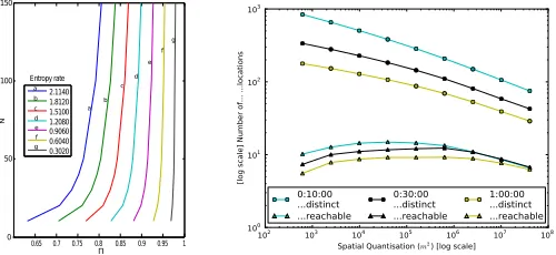
Recall that the main correction we have made to the approach in [1] is to address its assignment of a positive “next step” probabilities to all locations - even those impossible to reach. The magnitude of the corrective effect we implement is therefore dependent on the difference between the number of all possible (distinct) locations,N, and the number of locations that are reachable in reality, Nr since Π is monotonically

increasing in Nx via HF(Π, Nx) (see Fig. 2). Since the

number of reachable locations differs depending on the current location, the maximum number of reachable (i.e. non-zero probability) locations across all possible choices of “current

0.65 0.7 0.75 0.8 0.85 0.9 0.95 1 0

50 100 150

N

2.1140 1.8120 1.5100 1.2080 0.9060 0.6040 0.3020 Entropy rate

Π

a a b c d e f g

b c

d e

f g

Fig. 2. Plot showingΠ&Nin

HF(Π, N)inc. monotonically.

102 ₁₀3 ₁₀4 ₁₀5 ₁₀6 ₁₀7 ₁₀8 Spatial Quantisation (m2_{) [log scale]}

100 101 102 103

[log scale] Number of... ...locations

0:10:00 ...distinct ...reachable

0:30:00 ...distinct ...reachable

1:00:00 ...distinct ...reachable

Fig. 3. Graph showing the number of distinct locations vs reachable locations

location” is used so as to not underestimate the number of possible reachable locations, and maintain the upper bound. Formally Nr is calculated from an empirical symbolic time

seriesT ={s1, s2, . . . , sm}, with the set of all possible spatial

locations being Ω, as Nr = maxx∈Ω|{si+1 : si =x}|. This

is a per-individual, data-driven over-estimation of reachability. Importantly, this data-driven approach prevents the arbitrary over-estimation of possible “next-step” locations, which occurs when techniques such as grid based reachability, unperson-alised “ground cover” maps2 _{(e.g. [20]) or arbitrarily sized}

sets of data-driven possible locations3 (as previously used in [1] and subsequent work) are used.

An important empirical observation is that in using more fine-grained spatial quantizations one significantly increases the difference between N andNr. This difference, based on

examining all trajectories from the Geolife dataset [10], is shown as a log-log plot in Fig. 3 highlighting not only a significant difference between N andNr in general, but also

that this difference is particularly pronounced for more fine-grained spatial quantization levels. As such it is expected (and validated in section VI-C) that the difference between the upper bound calculated by the original formula from [1] and the refined upper bound calculated via this work will be more pronounced for higher spatial quantizations.

VI. AN EMPIRICAL EVALUATION

In this section we implement both the original [1] and our new method for calculating an upper limit for predictability and test it on real world data. The sensitivity of these limits to both temporal and spatial resolution is also investigated. In order to aid replicability a supporting website is available4_.

A. Dataset

The Geolife dataset [16] contains 182 individual’s GPS trajectories (longitude/latitude points, points omitted when no GPS was available) of varying lengths and sampling rates over a period of five years. Because many individuals have an insufficient number of data points to obtain an accurate estimate of their entropy, we are only able to consider data for a subset of individuals in our analysis. To determine individuals with sufficient data we calculated the entropy rate estimate

for every individual. If this value fell above the theoretical maximum entropy rate5, then the corresponding individual was not selected. Of the remaining individuals, plots of the estimated entropy rate as a function of time were studied. Those exhibiting obvious signs of non-convergence were not selected6_{. This left a group of 42 individuals}7_{. However, it}

was not possible to use the whole set of 42 individuals at all spatiotemporal quantizations considered. In particular, far more data is required to even approximately estimate the entropy rate of an individual when combining a fine-grained spatial quantization with a coarse fine-grained temporal quantization (because coarse grained temporal quantization results in a reduced number of points and fine-grained spatial quantization results in significantly more unique locations and hence lower repeating patterns). Instances where this occurred are clearly marked in the results and are discussed accordingly. In this way, we are able to quantitatively examine the majority of spatiotemporal quantizations, and treat any quantization levels which are restricted to a small sample of individuals in a more qualitative fashion.

B. Methodology

As detailed in section IV, an upper bound on predictability can be estimated from symbolised versions of individuals’ historic movement logs. To symbolise the GPS data a hier-archical, equal area quantization of the Earth is used [21]. Each individual’s upper bound on the maximum predictability is calculated using both the original method proposed by [1] and our new method. The mean across all individuals is then reported, before iterating for each combination of spatial and temporal quantization level. Spatial quantization levels of 618m2_{, 2474m}2_{, 9896m}2_{, 39586m}2_{, 158347m}2_{, 633388m}2_,

2.53km2, 10.13km2, 40.54km2 along with temporal quanti-zation levels of 5,10,15,30,45 and60minutes were investi-gated. These spatial and temporal quantizations reflect a similar range of quantizations to that previously considered in [3], [4]. Note that more fined-grained spatial quantization is likely to lead to inaccuracies due to GPS error and higher temporal quantizations are unlikely to provide enough data.

When calculating the empirical entropy rate we use the following estimator8 _{based on Lempel-Ziv data compression}

[18], where T is an individual’s observed time-series(that we model as having been generated by the stochastic process X) andΛiis the length of the longest pattern that starts at position

i, but which has not been seen prior to that point. It has been proven that the estimateHˆ(X)converges to the actual entropy rate, H(X), when tapproaches infinity [18].

ˆ

H(X) =H(T) =1_tPt i=2

Λi(T)

log₂i −1

(15)

C. Results and Discussion

Our results are shown via the three heatmaps in Fig. 4, and empirically confirm that our method not only achieves

5_{Due to the entropy rate definition,H(X), and lemma 1 this islog}

2(Nr).

6_{Typically due to a low number of data points.}

7_{Specifically, we used individuals with ids: 0-5,7,9,12-17,22,24,28,30,35,36,}

38-40,43,44,50,52,55,68,71,82,84,85,92,96,101,104,119,126,153,167,179.

8_{We note this estimator, used in [3], is slightly different to that used by}

[1]. While both estimators converge to the same value in the limit preliminary experiments on synthetic data suggested the former converges faster.

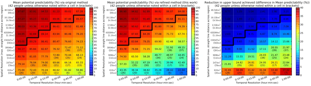
a tighter upper bound than the original approach in [1] in all circumstances, but that this improvement is sizeable especially at finer grained levels of quantization. The heatmaps compare:

(left)the mean upper bound on the maximum predictability as

computed by the original method from [1];(middle)the mean upper bound as computed by the refined method presented in this work; and (right) the mean difference between the two approaches. In all cases these values were computed over the six temporal quantizations and nine spatial quantizations.

All three heatmaps include a black line, above which cells denote spatiotemporal quantizations which a person could not walk across within a single timestep9. This is of interest since quantizations above this line have a clear advantage with respect to “next step” prediction. The reason for this is that, while the dataset contains a variety of transportation types, a non-trivial number of trajectories were undertaken on foot10. In these trajectories, many “next-steps” will be to the same region as the one they are currently in. Hence, a prediction of “no movement” will automatically be correct a predominant amount of the time, solely as a consequence of the granularity chosen. As such spatiotemporal quantizations below this line are often of greater interest. Fig. 4, (left), shows the mean upper bound of predictability over all individuals as computed by the original approach. This acts as a baseline to consider the magnitude of the refinement provided by our new formulation. Results are, as expected, slightly lower than prior work. This is to be expected as we focus on next-location predictability only within trajectories (see section III) - and this means we do not include a comparatively large amount of non-movement, which is easier to predict. At the same quantization levels used in the original work of [1], we report a predictability limit of between 81.45-85.57%, compared to the 93%they reported.

We also compare our results with [3]. At the finest spatial resolution used in that study of 350,000m2_{, at a five minute}

temporal resolution, an upper bound of≈98.5%was reported compared to our 93.05-94.7%. While this is relatively close, as the temporal quantization becomes more coarse the differ-ence increases substantially - where [3] reports ≈91.7%, at an hour spatial quantization, we report 74.23-78.20%. Such differences, however, are well within expectations - when an individual is sampled at a coarse temporal granularity the uncertainty of their location increases significantly, and this is only emphasized when non-movement is not considered. We note also that these differences have no effect on our subsequent analysis, as this result set remains a cogent baseline against which we can compare the impact of our new method. However, it does emphasize (even before the application of a refined approach to calculating the upper bound of predictabil-ity), that previously reported upper bounds are inflated due to the inclusion of significant amounts of non-movement.

Our main contribution is illustrated in Fig. 4, middleand

right, which highlight the importance of incorporating

topo-logical constraints in calculating upper bounds on maximum predictability. Across all quantization levels an average refine-ment of 12.9% was achieved (with a refinement of 17.69% achieved for quantizations below the black line). Excluding the combinations which could not include all 42 individuals

0:05:00 0:10:00 0:15:00 0:30:00 0:45:00 1:00:00

Temporal Resolution (hour:min:sec)

618m2 (35m)

2474m2 (70m)

9896m2 (141m)

39586m2 (281m)

158347m2 (563m)

633388m2 (1.1km)

2.53km2 (2.3km)

10.13km2 (4.5km)

40.54km2 (9km)

Spatial Resolution (max. straight line distance across region)

75.00

(26) 72.43(20) 70.24(15) 66.62(11) 61.82(6) 59.86(7) 79.14 76.04₍₃₅₎ 74.00₍₃₀₎ 69.66₍₂₁₎ 66.16₍₁₇₎ 65.33₍₁₅₎ 85.78 81.05 77.79 72.80₍₃₄₎ 70.44₍₂₅₎ 68.13₍₂₄₎ 90.17 85.84 82.67 76.32 72.47₍₃₉₎ 71.12₍₃₇₎ 93.05 89.29 86.41 80.47 76.60 74.23 94.85 91.69 89.14 83.94 80.48 78.20 96.03 93.36 91.19 86.61 83.52 81.48 97.27 95.27 93.61 89.96 87.46 85.57 97.67 95.91 94.53 91.23 89.02 87.28

Mean potential predictability (%) via original method (42 people unless otherwise noted within a cell in brackets)

0 5 10 15 20 25 30 35 40 45 50 55 60 65 70 75 80 85 90 95 100

0:05:00 0:10:00 0:15:00 0:30:00 0:45:00 1:00:00

Temporal Resolution (hour:min:sec)

618m2 (35m)

2474m2 (70m)

9896m2 (141m)

39586m2 (281m)

158347m2 (563m)

633388m2 (1.1km)

2.53km2 (2.3km)

10.13km2 (4.5km)

40.54km2 (9km)

Spatial Resolution (max. straight line distance across region)

43.35

(26) 38.34(20) 38.82(15) 35.28(11) 28.42(6) 22.84(7) 57.33 51.22₍₃₅₎ 47.19₍₃₀₎ 44.71₍₂₁₎ 39.96₍₁₇₎ 42.49₍₁₅₎ 74.50 65.50 58.28 48.77₍₃₄₎ 48.97₍₂₅₎ 44.65₍₂₄₎ 83.78 76.84 71.15 59.22 51.92₍₃₉₎ 49.15₍₃₇₎ 89.16 83.64 79.35 69.90 62.48 58.57 92.23 87.83 84.39 77.08 71.73 67.74 94.24 90.62 87.85 81.80 77.38 74.39 96.25 93.57 91.49 86.86 83.68 81.11 96.90 94.62 92.89 88.82 86.07 84.08

Mean potential predictability (%) via refined method (this work) (42 people unless otherwise noted within a cell in brackets)

0 5 10 15 20 25 30 35 40 45 50 55 60 65 70 75 80 85 90 95 100

0:05:00 0:10:00 0:15:00 0:30:00 0:45:00 1:00:00

Temporal Resolution (hour:min:sec)

618m2 (35m)

2474m2 (70m)

9896m2 (141m)

39586m2 (281m)

158347m2 (563m)

633388m2 (1.1km)

2.53km2 (2.3km)

10.13km2 (4.5km)

40.54km2 (9km)

Spatial Resolution (max. straight line distance across region)

31.65

(26) 34.09(20) 31.42(15) 31.34(11) 33.40(6) 37.02(7) 21.81 24.82₍₃₅₎ 26.81₍₃₀₎ 24.95₍₂₁₎ 26.21₍₁₇₎ 22.84₍₁₅₎ 11.29 15.55 19.51 24.03₍₃₄₎ 21.47₍₂₅₎ 23.48₍₂₄₎ 6.39 9.00 11.52 17.11 20.55₍₃₉₎ 21.97₍₃₇₎ 3.90 5.65 7.05 10.57 14.12 15.66 2.63 3.86 4.75 6.87 8.74 10.46 1.78 2.73 3.34 4.82 6.14 7.09 1.02 1.69 2.11 3.10 3.78 4.46 0.77 1.29 1.64 2.41 2.96 3.21

Reduction in upper bound achieved (difference in Mean predictability (%)) (42 people unless otherwise noted within a cell in brackets)

0 5 10 15 20 25 30 35 40

Fig. 4. Predictability upper bound results for varying spatiotemporal quantizations. Dark black line separates the spatiotemporal quantizations one can cross within one time period walking (those below the line) at the preferred walking speed of 5km/hour [22]. LEFT: Predictability upper bounds as defined in [1]. MIDDLE: Predictability upper bounds as defined in this work. RIGHT: Difference in predictability upper bounds between the two methods.

(due to the extra data requirements at fine-grained levels) the average refinement was still 10.4%for the combinations below the line and 6.86%including those above.

However, the corrections to upper bounds of human pre-dictability are particularly of note when the spatial quanti-zation is fine-grained - the level relevant to a large number of interesting pervasive applications (e.g. location-sensitive advertising [5] or detecting route errors [8]). Specifically, the average refinement of the upper bound achieved in this work is between 10-24% for a spatial quantization of 9896m2, 21-26% for 2474m2 _{and 31-37% for 618m}2_{. While these}

figures are not always supported by a sample size as large as 42 individuals they do help to show a strong trend in results: as temporal quantization becomes coarser, and spatial quantization becomes finer our approach has a greater impact on the upper bounds of maximum predictability. These results also match the expectations from the theory discussed in section V.

Considering the absolute values in Fig. 4,(centre), it is of note that the refined upper bound varies quite substantially. Of particular interest is when the upper bound is low. This is because, as an upper bound, the value only denotes that one cannot create a predictor that performs better - not that it is possible in reality to create one that reaches that level of performance. As such high bounds are of limited value, and should serve only as encouragement to researchers by hinting at the possibility of better predictive algorithms. In contrast low values provide an explicit indication that movement data alone will likely not achieve research and/or industry goals with regard to prediction.

The lowest upper bound of 22.84%occurs under the finest spatial quantization level (618m2_{) and at the coarsest temporal}

quantization level. While the lower number of individuals con-tributing to the average means that this particular result must be taken with caution, the general trend indicates that attempting prediction at this, or any finer (coarser), spatial (temporal) granularity is unlikely to provide useful performance based on locational trails alone. For a significant number of applications which require high levels of predictability to function (such as ones where predictions will directly result in user interaction) this statement applies to allconsidered temporal quantization

levels at the spatial granularity of 618m2(and likely 2474m2) because at those levels even the best possible prediction algorithm will only be correct 57.33% of the time (which seems insufficient to support a robust service). In fact, out of all the spatiotemporal quantization levels considered that individuals could cross on foot, and hence not introducing systematic bias due to the analysis of next step predictability, only 35% (14/37) had an upper bound of more than 70%.

While the low predictability limits highlighted in this work have potential to cast doubts on the use of predictive algorithms based on human movement traces, at least for prediction with spatial granularity less than 9896m2, it is important to realise that it does not preclude advances beyond these limits through the incorporation of other information sources into prediction. Indeed, such systems have been advocated for numerous years, empirically outperforming systems relying on singular information sources. As such these results contribute solid evidence that such systems will be required if performance targets are desired beyond the values reported in Fig. 4. A final point to remember is that these are mean upper bounds. Some individuals and/or groups will have higher predictability, particularly in some datasets (e.g. as discussed in [2]).

VII. CONCLUSION

In this work we reconsidered the derivation of the upper bound of the maximum (upper limit) predictability of human mobility. Previous results based on a method for computing the upper bound by [1] have suggested high predictability at or above 90% across a range of spatiotemporal quantization levels. Noting an overestimation of the bound in the formula-tion in [1], due to a lack of topological constraints, an alternate formulation is provided which is shown both theoretically and empirically to provide a lower, and therefore closer to the true, upper bound providing the opportunity to revisit the studies of [1]–[4].

can be lower than required for many real world applications (e.g. 57.33% under a spatial quantization of 2474m2 and 5 minute sampling). Furthermore, a strong trend is evident that this gets worse as temporal sampling rates are reduced and the predictions are made over a longer time window. Such results provide an important, sobering, look at the role of movement traces for predicting users locations, indicating that on their own (and without integration of further external knowledge) they will not provide sufficient foundation. These results therefore provide solid evidence that in these cases prediction algorithms should either: use a different approach completely (i.e. approaches following different definitions of prediction or mobility); focus on delineating sub-populations with exceptionally regular behaviour; or integrate external variables in order to achieve the desired prediction accuracy to meet the applications performance needs.

ACKNOWLEDGEMENTS

The authors would like to thank our shepherd Silvia Santini and the anonymous reviewers for their valuable comments. This work was funded by the RCUK Horizon Digital Economy Research Hub grant, EP/G065802/1.

APPENDIXA

PROOF OFTHEOREM1:H(Xn|hn)≤HF(π)

This proof makes explicit the claim in [17, p12] that H(Xn|hn)≤HF(π)“represents an appropriate rewritting of

Fano’s inequality”.

Proof: Consider the optimal prediction algorithm, which

will always predictxM L. A prediction error occurs when this

prediction differs from the individuals actual move (i.e). Let us define the probability of this event as P(e), and denote its associated binary entropy as H(E). Correspondingly:

P(xM L|hn) =π= 1−P(e|hn) (16)

By Fano’s inequality [19]:

H(Xn|hn)≤H(E|hn) +P(e|hn) log2(N−1) (17)

Substituting 16 into 17:

H(Xn|hn)≤ −πlog2π−(1−π) log2

1−π N−1

(18)

Since RHS of Eq. 18 equals Eq. 6:H(Xn|hn)≤HF(π)

APPENDIXB PROOF OFLEMMA1

Proof: Consider a distributionP(X)with a setV of Nr

non-zero outcomes and a set Z of Nz zero outcomes.

H(X) =Pv∈V P(v) log2P1(v)+

P

z∈ZP(z) log2P(1z) (19)

≤ log₂P

v∈V P(v)

1

P(v) (20)

= log2|V|= log2Nr (21)

Eq. 19 is by the definition of entropy, Eq. 20 by the fact that when calculating entropy 0 log₂(0)is taken to be zero and by definition all P(z) = 0 with the inequality due to Jensen’s inequality sincelog₂xis strictly convex [23].

REFERENCES

[1] C. Song, Z. Qu, N. Blumm, and A.-L. Barabsi, “Limits of predictability in human mobility,”Science, vol. 327, no. 5968, pp. 1018–1021, 2010. [2] B. Jensen, J. Larsen, K. Jensen, J. Larsen, and L. Hansen, “Estimating human predictability from mobile sensor data,” inIEEE Int’l Workshop Machine Learning for Signal Processing (MLSP), 2010, pp. 196–201. [3] M. Lin, W.-J. Hsu, and Z. Q. Lee, “Predictability of individuals’ mobility with high-resolution positioning data,” in Proc. ACM Conf. on Ubiquitous Computing (UBICOMP). ACM, 2012, pp. 381–390.

[4] W. Qian, K. Stanley, and N. Osgood, “The impact of spatial resolution and representation on human mobility predictability,” inInt’l Workshop Web & Wireless Geographical Information Systems. Springer, 2013. [5] J. Krumm, “Ubiquitous advertising: The killer application for the 21st

century,”Pervasive Computing, IEEE, vol. 10, no. 1, pp. 66–73, 2011. [6] B. Jung, M. Choi, H. Youn, and O. Song, “Vertical handover based on the prediction of mobility of mobile node,” inIEEE Int’l Conf. Pervasive Computing and Communications Workshops, 2010, pp. 534–539. [7] J. Froehlich and J. Krumm, “Route prediction from trip observations,”

SAE SP, vol. 2193, p. 53, 2008.

[8] D. Patterson, L. Liao, K. Gajos, M. Collier, N. Livic, K. Olson, S. Wang, D. Fox, and H. Kautz, “Opportunity knocks: A system to provide cognitive assistance with transportation services,” inProc. ACM Conf. on Ubiquitous Computing (UBICOMP), 2004, pp. 433–450.

[9] B. D. Ziebart, N. Ratliff, G. Gallagher, C. Mertz, K. Peterson, J. A. Bagnell, M. Hebert, A. K. Dey, and S. Srinivasa, “Planning-based prediction for pedestrians,” inIEEE/RSJ Int’l Conf. Intelligent Robots and Systems (IROS). IEEE, 2009, pp. 3931–3936.

[10] Y. Zheng, L. Zhang, X. Xie, and W.-Y. Ma, “Mining interesting locations and travel sequences from gps trajectories,” inProc. Int’l Conf. World Wide Web (WWW). ACM, 2009, pp. 791–800.

[11] Y. Chon, H. Shin, E. Talipov, and H. Cha, “Evaluating mobility models for temporal prediction with high-granularity mobility data,” in Int’l Conf. Pervasive Computing and Communications, 2012, pp. 206–212. [12] W. Mathew, R. Raposo, and B. Martins, “Predicting future locations

with hidden markov models,” in Proc. ACM Conf. on Ubiquitous Computing (UBICOMP). ACM, 2012, pp. 911–918.

[13] P. Baumann, W. Kleiminger, and S. Santini, “The influence of tem-poral and spatial features on the performance of next-place prediction algorithms,” in Proc. ACM Int’l Conf. on Pervasive and Ubiquitous Computing (UbiComp). New York, NY, USA: ACM, 2013, pp. 449– 458.

[14] S. Scellato, M. Musolesi, C. Mascolo, V. Latora, and A. Campbell, “Nextplace: A spatio-temporal prediction framework for pervasive sys-tems,” inInt’l Conf Pervasive Computing. Springer, 2011, pp. 152–169. [15] A. Monreale, F. Pinelli, R. Trasarti, and F. Giannotti, “Wherenext: a location predictor on trajectory pattern mining,” in Proc Int’l Conf Knowledge discovery & data mining (KDD). ACM, 2009, pp. 637–646. [16] Microsoft Research. Geolife dataset and user guide: 1.3. [Online].

Available: http://research.microsoft.com/en-us/downloads/

[17] C. Song, Z. Qu, N. Blumm, and A.-L. Barabsi. (2010) Limits of predictability in human mobility (supporting material). [Online]. Available: www.sciencemag.org/content/327/5968/1018/suppl/DC1 [18] I. Kontoyiannis, P. Algoet, Y. Suhov, and A. Wyner, “Nonparametric

entropy estimation for stationary processes and random fields, with applications to english text,” Information Theory, IEEE Transactions on, vol. 44, no. 3, pp. 1319–1327, 1998.

[19] R. Fano, “Fano inequality,”Scholarpedia, vol. 3, no. 10, p. 6648, 2008. [20] J. Krumm and E. Horvitz, “Predestination: Where do you want to go

today?”Computer, vol. 40, no. 4, pp. 105–107, 2007.

[21] K. G´orski, E. Hivon, A. Banday, B. Wandelt, F. Hansen, M. Reinecke, and M. Bartelmann, “Healpix: A framework for high-resolution dis-cretization and fast analysis of data distributed on the sphere,” The Astrophysical Journal, vol. 622, no. 2, p. 759, 2005.

[22] J. Rose, H. Ralson, and J. Gamble, “Energetics of walking,” inHuman walking. Williams & Wilkins, 1994, pp. 45–72.