Munich Personal RePEc Archive
The role of component-wise boosting for
regional economic forecasting
Lehmann, Robert and Wohlrabe, Klaus
Ifo Institute, Dresden, Ifo Institute, Munich
3 December 2015
Online at
https://mpra.ub.uni-muenchen.de/68186/
The role of component-wise boosting for
regional economic forecasting
Robert Lehmann
∗Klaus Wohlrabe
†This version: December 3, 2015
Abstract. This paper applies component-wise boosting to the topic of regional economic forecasting. By using unique quarterly gross domestic product data for one German state for the period from 1996 to 2013, in combination with a large data set of 253 monthly indicators, we show how accurate forecasts obtained from component-wise boosting are compared to a simple benchmark model. We additionally take a closer look into the algorithm and evaluate whether a sta-ble pattern of selected indicators exists over time and four different forecasting horizons. All in all, boosting is a viable method for forecasting regional GDP, especially one and two quarters ahead. We also find that regional survey results, indicators that mirror the Saxon economy and the Composite Leading Indicators by the OECD, get frequently selected by the algorithm.
Keywords: boosting; regional economic forecasting; gross domestic product
JEL-Classification: C53; E17; E37; R11
∗Corresponding author. Ifo Institute – Leibniz-Institute for Economic Research at the University of
Mu-nich e.V., Dresden Branch, Einsteinstr. 3, D-01069 Dresden. Phone: +49(0)351/26476-21. Email: [email protected]. Acknowledgments: We thank Lisa Giani Contini for editing this text.
†Ifo Institute – Leibniz-Institute for Economic Research at the University of Munich e.V., Poschingerstr.
1. Introduction
The topic of regional economic forecasting is increasingly becoming part of literature in this field in recent years. A recent survey by Lehmann and Wohlrabe (2014b) discusses state-of-the-art methodology in regional economic forecasting and names possible future research activities in this field. One of such activities could be examining the forecasting performance of boosting algorithms for regional economic development. In this paper, we fill this gap in the existing literature by making two contributions. Firstly, we generally ask whether boosting produces lower forecast errors for regional gross domestic product compared to a benchmark model. And secondly, we follow the papers by Lehmann and Wohlrabe (2015b) and Kim and Swanson (2014) that take a closer look into the boosting procedure. To be more precise, we ask whether there are superior indicators for regional economic forecasting that get selected into the model by the algorithm. The paper is organized as follows: Section 2 introduces the boosting algorithm. In Section 3 we first present our data, followed by the forecasting methodology and a discussion of the results. The final section offers some conclusions.
2. Boosting Algorithm
This paper applies the L2-boosting approach also used in the corresponding literature (see
Buchen and Wohlrabe, 2011; Lehmann and Wohlrabe, 2015b; Pierdzioch et al., 2015a,b). Generally, boosting follows the idea of iteratively estimating an unknown function in either a linear or nonlinear manner. In applications with large data sets (N ≥T), the complexity of the chosen fitting procedure has to be reduced by a pre-selection of variables (Bühlmann and Yu, 2003). Therefore, component-wise boosting estimates a generalized model in additive form. We choose the standard autoregressive distributed lag (ADL) model:
E(yt|zt, δ) =: F(zt, δ) = δ′
zt
= α+β1yt−h+ N
X
j=1
γjxjt−h . (1)
The vector z= (y, x1, . . . , xN) comprises the lagged target variable to predict (y) and all lagged exogeneous predictors (x). We restrict our analysis to allow only a h-period lag of y
or xj. Therefore, the number of exogeneous variables is denoted by N. All variables that are not selected by the algorithm obtain a zero restriction. We apply the standard squared error loss (L2) in order to decide the selection:
L(yt, F(zt, δ)) = 1
2(yt−F(zt, δ))
2 (2)
From the pool ofk = 1+N potential predictorszk, the algorithm chooses in every iteration
m one variable zk∗
m that yields the smallest sum of squared residuals (SSR). But it is worth noting that the chosen predictor in a specific iteration does not have to be necessarily different from those of previous iterations. As the fitting procedureF(.) in every iteration (called base learner) we apply ordinary least squares (OLS) for a linear model. The algorithm proceeds as follows:
1. Initialize fbt,0(.) = y for each t. Set m = 0.
2. Increasemby 1. Fort = 1, . . . , T, compute the negative gradient−∂L(∂Fyt,F)and evaluate atfbt,m−1(zt,δb[m−1]): ut=yt−fbt,m−1(zt,δb[m−1]).
3. Fork = 1, . . . ,1+N, regress the negative gradient vectoruonzk and computeSSRk =
PT
t=1(ut−zt,kθbk)2. 4. Choose zk∗
m such that SSRkm∗ = arg mink∈NSSRk. 5. Let fbt,m(.) =zt,k∗
mθbkm∗.
6. For t = 1, . . . , T, update fbt,m(.) = fbt,m−1(.) +νfbt,m(.), where 0< ν <1.
7. Iterate steps 2 to 6 until m =M∗
.
From steps 2 and 3 it immediately follows that L2-loss-boosting is just a repeated least
squares fitting of residuals. The algorithm converges to a function that represents the sum of M∗
base learner estimates multiplied by the constant shrinkage parameter ν:
b
F(zt,δb[M ∗]
) = M∗
X
m=0
νfbm(zt,θb[m]) . (3)
The optimal number of iteration steps M∗
minimizes the expected forecast error either estimated by cross-validation or by an information criterion. Friedman (2001) first introduces
ν as an additional regularization parameter next tom. The main reason for the introduction is to reduce the learner’s variance, thus, improving the prediction performance of boosting.
3. Boosting and Regional Economic Forecasting
3.1. Data
National accounts data for regional entities such as counties or districts are generally only available on an annual basis. Since large data set methods such as boosting only work with
a sufficient number of observations, annual information is not suitable for our purposes. However, as in Lehmann and Wohlrabe (2014a, 2015a), we can rely on quarterly gross domestic product (GDP) data for one of the sixteen German states: the Free State of Saxony. Saxony is part of the Eastern German states that joined Germany after its reunification in 1989. Compared to all German states, the Free State of Saxony had the eighth largest share of total nominal German GDP in 2014 (≈ 4%). If we focus on Eastern Germany (without Berlin) instead, Saxony has the highest nominal GDP compared to all of the other Eastern German states. Additionally, the Free State of Saxony is the Eastern German state with the highest industrial share and the largest export quota. Taking all these factors into account makes the Free State of Saxony an interesting object to study.
The quarterly data used in this paper are not published by official statistics, but rather by an academic research institute: the German Ifo Institute. The calculations are based on a temporal disaggregation procedure that applies a stable relationship between the target series and a suitable indicator. Details on the procedure can be found in Nierhaus (2007). This paper uses real quarterly GDP data for the period from 1996Q1 to 2013Q4. The series is seasonally adjusted and we apply a quarter-on-quarter growth rate transformation to reach stationarity, as well as to capture the business cycle of the series.
We apply the boosting algorithm to a data set that contains 253 monthly indicators. This data set is predominantly the same as in Henzel et al. (2015). In order to systematize the indicators, we group them into six categories: macroeconomic (72), finance (20), prices (11), surveys (56), international (25) and regional (69). The indicators from the first four categories are measured at the national level (here: Germany). Since Saxony has an open economy, we expect international indicators to deliver useful information to forecast Saxon GDP. In order to capture region-specific developments, we add indicators that are measured at the regional level (here: Saxony). It is worth mentioning that we generally exclude those indicators that were used for temporal disaggregation of the GDP figures. All indicators are also seasonally adjusted. Since the potential predictors are measured on a monthly basis, we apply a three-month-average to obtain quarterly data. Whenever indicators are not stationary in levels, we either calculate quarter-on-quarter growth rates or first differences.
3.2. Forecasting Approach
We generate forecasts for the h-step ahead quarter-on-quarter growth rate of Saxon GDP, where h stands for the forecast horizon: h = 1,2,3 and 4 quarters. The forecasts are gen-erated directly and pseudo out-of-sample with an expanding window. The initial estimation window ranges from 1996Q1 to 2003Q4 and is successively enlarged by one quarter in every iteration. The first forecast is obtained for the first quarter 2002. As the standard measure of forecast accuracy, we use the relative root mean squared forecast errors (rRM SF Es), where a boosted autoregressive process of order one serves as the benchmark model:
E(yt+h|yt) =α+β1yt−h (4)
For the boosting procedure, OLS serves as the base learner and we apply an L2-loss
function. The model is selected according to the corrected Akaike Information Criterion (see Buchen and Wohlrabe, 2014) with a maximum number of 15 iterations (mmax = 15). We have to apply these criteria because of the shortness of the Saxon GDP series. All other parameters are optimally chosen.
3.3. Results
In general, component-wise boosting does a good job of predicting Saxon GDP growth. For
h= 1,2 and 4 the rRM SF Esare 0.910, 0.978 and 0.990, thus, the boosted indicator model beats the autoregressive benchmark. The ratio is only slightly larger than one (1.055) for
h = 3. Thus, the most precise forecasts can be generated in the short run. The number of indicators that get chosen by the procedure is very stable over time. Figure 1 shows the number of selected indicators for each forecasting horizon and each quarter for which we generate a forecast. The four panels are perfectly comparable since they display a common
x-axis, as well as y-axes ranging from zero to ten.
The number of selected indicators forh = 1 rises over time, starting with four indicators in the model and ending up with eight predictors. For h = 2 the opposite holds: the number of selected indicators decreases with time. The most stable pattern with the lowest standard deviation in selected indicators shows up forh= 3. As for predictions two quarters ahead, the number of selected indicators decreases for the longest forecast horizon. Another interesting observation is that the global economic crisis of 2008/2009 deteriorates the picture of indicator selection.
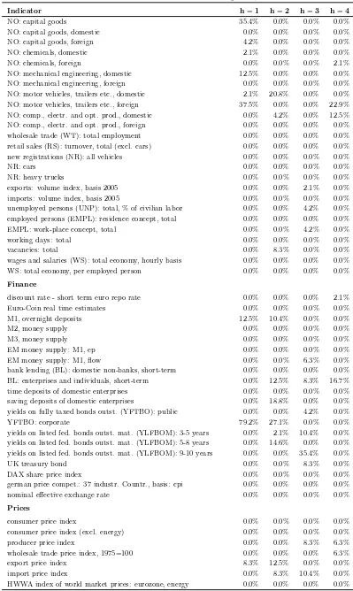
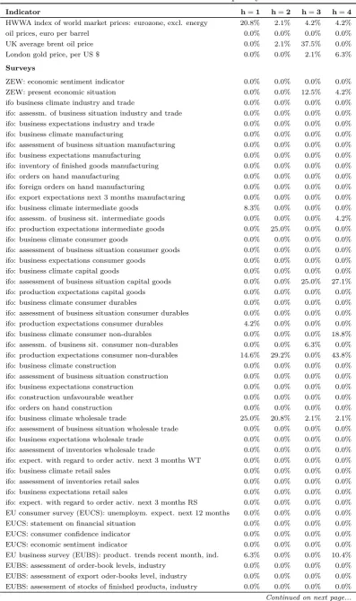
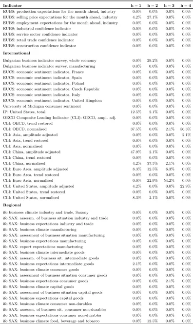
Our next step is to ask whether there are some indicators that get regularly selected by the algorithm. We can generally state that the composition of best indicators varies with the forecast horizon. However, there are indicators that show up for almost all horizons. At the opposite end of the scale, we have indicators in the sample such as price indices that never get selected by the procedure.1 The most regularly chosen indicators are measured
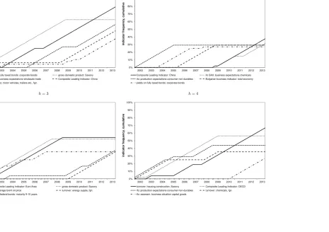
at the regional level, or are provided by the OECD in terms of their Composite Leading Indicators (CLI). In order to determine the most frequently chosen indicators, we introduce the following Figure 2 that shows the top five for each forecast horizon. The four panels can be interpreted in the same way. Our forecasting period in quarterly frequency is displayed on the x-axes. The y-axes show the cumulative frequency of an indicator that has been chosen by the boosting algorithm. Thus, the y-axes run from 0% to 100%. If an indicator gets chosen in period t, then the cumulative frequency rises by 1/48, with 48 as the length of our forecasting period. In other words, the slope of each line is 2.08 percentage points.
1A complete list of all indicators and their relative frequency can be found in Table 2 in Appendix A.
An indicator’s total frequency is then the sum of all forecasting steps where the indicator is part of the boosting model, divided by the length of the evaluation period. If the indicator is part of the boosting model in each point in time, the resulting line will be a 45°-line. If there are phases where the indicator has not been chosen by the procedure, then the line takes a horizontal course.
The most frequent selected indicator forh = 1 are yields on fully taxed bonds, followed by autoregressive terms of the target variable and Ifo business expectations for Saxon wholesal-ing. We find similar results as in Lehmann and Wohlrabe (2014a), where government bond yields as well as the Ifo business expectations for Saxon wholesaling played a crucial role in forecasting total Saxon gross value added. Another interesting result is that foreign new orders of motor vehicles and trailers in Germany get frequently selected by the algorithm forh = 1. Such a result is straightforward and in line with Henzelet al.(2015). The vehicle manufacturing sector is the most important for the Saxon economy. In 2014, almost 30% of total Saxon industrial turnover was generated in the vehicle manufacturing sector. Un-fortunately, official statistics provide no long time series on new orders of the Saxon vehicle manufacturing sector. We suggest that such an indicator will be selected very frequently by the algorithm.
For h = 2 the most frequent selected indicator is the OECD CLI for China, followed by a regional and a national survey indicator of the Ifo Institute. The OECD CLI for China is also among the top five for the shortest forecast horizon. China plays a crucial role for Saxon firms. In 2014, almost 18% of all Saxon exports were demanded by China, followed by the United States with a share of approximately 10% and Poland with 5%. In general, the Saxon economy has the highest export quota (2014: ≈ 38% of total turnover in manufacturing were generated abroad) among the Eastern German states. Additionally, these results are in line with Henzel et al. (2015). As stated before, regional survey results (Ifo business expectations for the Saxon chemical industry) are part of the boosting model. This result is also straightforward, since the chemical industry has the fifth largest share (over 5% in 2014) of total manufacturing turnover in Saxony.
Turning to three quarter ahead predictions, we find the CLI for the Euro Area, the first lag of Saxon GDP and government bond yields among the five frequently selected indicators. These results are again in line with the existing literature (Lehmann and Wohlrabe, 2014a; Henzel et al., 2015). The finding that the economic development of the Euro Area has some predictive content in particular is obvious, since the Saxon economy exported almost the half of its goods to European member states in 2014.
Figure 1: Total number of selected indicators for each forecast horizon
h= 1 h= 2
9 10 8 6 7 indicator s 5 f selected 3 4 number o f 1 2 0 1
2002 2003 2004 2005 2006 2007 2008 2009 2010 2011 2012 2013 9 10 8 6 7 indicator s 5 f selected 3 4 number o f 1 2 0 1
2002 2003 2004 2005 2006 2007 2008 2009 2010 2011 2012 2013
h= 3 h= 4
9 10 8 6 7 indicator s 5 f selected 3 4 number o f 1 2 0 1
2002 2003 2004 2005 2006 2007 2008 2009 2010 2011 2012 2013 9 10 8 6 7 indicator s 5 f selected 3 4 number o f 1 2 0 1
2002 2003 2004 2005 2006 2007 2008 2009 2010 2011 2012 2013
Figure 2: Five most frequently selected indicators for each forecast horizon
h= 1 h= 2
40% 50% 60% 70% 80% 90% 100% di cator fr equency , cumul a ti v e 0% 10% 20% 30%
2002 2003 2004 2005 2006 2007 2008 2009 2010 2011 2012 2013
in
yields on fully taxed bonds: corporate bonds gross domestic product: Saxony ifo SAX: business expectations wholesale trade Composite Leading Indicator: China new orders: motor vehicles, trailers etc., fgn.
40% 50% 60% 70% 80% 90% 100% di cator fr equency , cumul a ti v e 0% 10% 20% 30%
2002 2003 2004 2005 2006 2007 2008 2009 2010 2011 2012 2013
in
Composite Leading Indicator: China ifo SAX: business expectations chemicals ifo: production expectations consumer non-durables Bulgarian business indicator: total economy yields on fully taxed bonds: corporate bonds
h= 3 h= 4
40% 50% 60% 70% 80% 90% 100% di cator fr equency , cumul a ti v e 0% 10% 20% 30%
2002 2003 2004 2005 2006 2007 2008 2009 2010 2011 2012 2013
in
Composite Leading Indicator: Euro Area gross domestic product: Saxony UK average brent oil price turnover: energy supply, fgn. yields federal bonds: maturity 9-10 years
40% 50% 60% 70% 80% 90% 100% di cator fr equency , cumul a ti v e 0% 10% 20% 30%
2002 2003 2004 2005 2006 2007 2008 2009 2010 2011 2012 2013
in
turnover: housing construction, Saxony Composite Leading Indicator: OECD ifo: production expectations consumer non-durables turnover: chemicals, fgn. ifo: assessm. business situation capital goods
For our longest forecast horizon (h = 4), we also find some interesting results. The most frequently selected indicators are turnover from Saxon housing construction, followed again by the CLI for the OECD and Ifo business survey results. The construction sector is tra-ditionally overrepresented in Eastern German states since large infrastructural investments were introduced after reunification (see Ragnitz, 2005) leading to a construction "boom". To stress the structure of the Saxon construction sector, housing construction accounted for a share of almost 26% of total construction turnover in 2014. Another highlight is the selection of the indicator Ifo assessment of the business situation of capital good producers. Next to intermediate good producers, the Saxon manufacturing sector is mainly described by capital goods producing firms (2014: share of 48% in total manufacturing turnover). As for the three forecasting horizons before, these two results are also in line with existing literature on the topic (Lehmann and Wohlrabe, 2015a).
After describing some overall results followed by the top five selected indicators, we take a closer look at the stability of the selection of indicators over time and forecasting horizons. Let us start with stability over time by looking at Figure 2 again. We can observe similar patterns between the shortest (h = 1) and longest (h = 4) forecast horizon, as well as for
h = 2 and h = 3. Whereas for the first pair of comparisons we find indicators that get selected over the whole forecasting period, for h= 2 and h= 3 there seems to be a break in the selection. Forh= 1 government bond yields get selected into the boosting model almost in each quarter; for h= 4 these are turnover for the Saxon housing construction sector. For
h = 2 and h = 3 there seems to be a break in the selection around the economic crisis of 2008/2009. By looking at forecasts of two quarters ahead, we see that, for example, the yields on fully taxed bonds get replaced by the CLI for China or the autoregressive term of the target variable around 2008. For h = 3 the CLI for the Euro Area gets replaced by foreign turnover in the sector of energy supply before the crisis. Henzel et al. (2015) also found that the crisis affects the performance of indicators, which makes this an interesting field of study. Due to the relatively small sample we cannot, however, elaborate more on such breaks at this point in time.
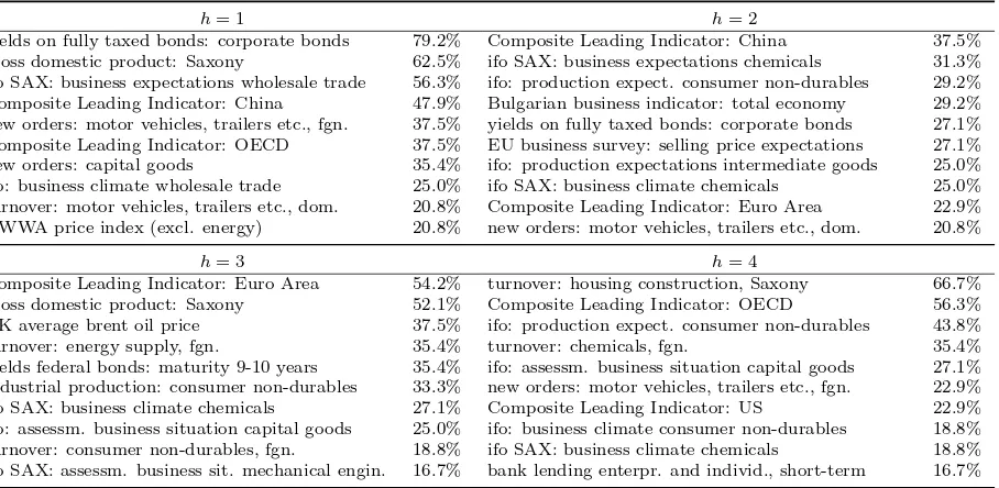
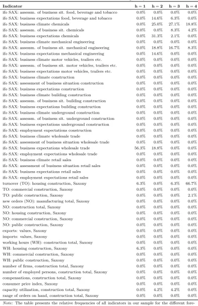
What about the selection stability of indicators over the different forecasting horizons? We answer this question by introducing the following Table 1 that shows the top 10 frequently selected indicators for all four forecasting horizons. The most frequently selected indicator for h = 1, yields on fully taxed bonds, is not part of the model for longer forecast horizons than two quarters ahead. Business expectations for the Saxon wholesale trade are only part of the model for one-quarter-ahead forecasts. Foreign new orders of motor vehicles etc. get selected into the model for h= 1 and h= 4.
Table 1: Top 10 indicators for each forecast horizon
h= 1 h= 2
yields on fully taxed bonds: corporate bonds 79.2% Composite Leading Indicator: China 37.5% gross domestic product: Saxony 62.5% ifo SAX: business expectations chemicals 31.3% ifo SAX: business expectations wholesale trade 56.3% ifo: production expect. consumer non-durables 29.2% Composite Leading Indicator: China 47.9% Bulgarian business indicator: total economy 29.2% new orders: motor vehicles, trailers etc., fgn. 37.5% yields on fully taxed bonds: corporate bonds 27.1% Composite Leading Indicator: OECD 37.5% EU business survey: selling price expectations 27.1% new orders: capital goods 35.4% ifo: production expectations intermediate goods 25.0% ifo: business climate wholesale trade 25.0% ifo SAX: business climate chemicals 25.0% turnover: motor vehicles, trailers etc., dom. 20.8% Composite Leading Indicator: Euro Area 22.9% HWWA price index (excl. energy) 20.8% new orders: motor vehicles, trailers etc., dom. 20.8%
h= 3 h= 4
Composite Leading Indicator: Euro Area 54.2% turnover: housing construction, Saxony 66.7% gross domestic product: Saxony 52.1% Composite Leading Indicator: OECD 56.3% UK average brent oil price 37.5% ifo: production expect. consumer non-durables 43.8% turnover: energy supply, fgn. 35.4% turnover: chemicals, fgn. 35.4% yields federal bonds: maturity 9-10 years 35.4% ifo: assessm. business situation capital goods 27.1% industrial production: consumer non-durables 33.3% new orders: motor vehicles, trailers etc., fgn. 22.9% ifo SAX: business climate chemicals 27.1% Composite Leading Indicator: US 22.9% ifo: assessm. business situation capital goods 25.0% ifo: business climate consumer non-durables 18.8% turnover: consumer non-durables, fgn. 18.8% ifo SAX: business climate chemicals 18.8% ifo SAX: assessm. business sit. mechanical engin. 16.7% bank lending enterpr. and individ., short-term 16.7%
Note:The table presents the relative frequencies of the top 10 indicators in our sample for the different forecasting horizons. A value of 100% is reached if an indicator gets chosen by the algorithm 48 times, thus, for the length of our forecasting period. An indicator is assigned with 0% if this indicator is not chosen over the forecasting period at all.
The Saxon chemical industry strongly contributes to the model selection: we find the Ifo Business Climate for the Saxon chemical industry ranks among the top 10 for two-quarter-ahead up to four-quarter-two-quarter-ahead forecasts. We always find a CLI among the top 10 for each forecast horizon. However, the countries or regions alternate between the forecasting horizons respectively. The most frequently selected indicator for h = 4, turnover in the Saxon housing construction sector, is only among the top 10 for this horizon.
4. Conclusion
With component-wise boosting we are able to calculate more precise forecasts of GDP for one German region compared to a simple benchmark model. A closer look into the boost-ing procedure reveals interestboost-ing results for regional economic forecastboost-ing. We can identify three major indicators or groups that get selected by the algorithm: regional survey results, indicators that mirror the Saxon economy and the Composite Leading Indicators released by the OECD. However, a large number of variables, such as price indices, are never part of the boosting model.
Since business cycle indicators like industrial production are not available at the regional level, future research activities can focus on variables like employment or the unemployment rate. These variables have one advantage in common: they are available at a monthly frequency. We expect different selection patterns to emerge. Against this backdrop, future research may also investigate possible breaks triggered by the economic crisis.
References
Buchen, T. and Wohlrabe, K. (2011). Forecasting with many predictors: Is boosting a viable alternative? Economics Letters, 113 (1), 16–18.
— and — (2014). Assessing the Macroeconomic Forecasting Performance of Boosting – Evidence for the United States, the Euro Area, and Germany. Journal of Forecasting,
33 (4), 231–242.
Bühlmann, P.andYu, B.(2003). Boosting with theL2loss: Regression and Classification. Journal of the American Statistical Association,98 (462), 324–339.
Friedman, J. H. (2001). Greedy Function Approximation: A Gradient Boosting Machine.
The Annals of Statistics, 29 (5), 1189–1232.
Henzel, S. R., Lehmann, R. and Wohlrabe, K. (2015). Nowcasting Regional GDP:
The Case of the Free State of Saxony.Review of Economics, 66 (1), 71–98.
Kim, H. H.andSwanson, N. R.(2014). Forecasting financial and macroeconomic variables using data reduction methods: New empirical evidence.Journal of Econometrics,178(2), 352–367.
Lehmann, R. and Wohlrabe, K. (2014a). Forecasting gross value-added at the regional level: are sectoral disaggregated predictions superior to direct ones? Review of Regional Research, 34 (1), 61–90.
—and —(2014b). Regional economic forecasting: state-of-the-art methodology and future challenges.Economics and Business Letters,3 (4), 218–231.
— and —(2015a). Forecasting GDP at the Regional Level with Many Predictors. German Economic Review,16 (2), 226–254.
— and —(2015b). Looking into the Black Box of Boosting: The Case of Germany. MPRA Paper No. 67608.
Nierhaus, W. (2007). Vierteljährliche Volkswirtschaftliche Gesamtrechnungen für Sachsen mit Hilfe temporaler Disaggregation. ifo Dresden berichtet,14 (4), 24–36.
Pierdzioch, C.,Risse, M.andRohloff, S.(2015a). A boosting approach to forecasting gold and silver returns: economic and statistical forecast evaluation. Applied Economics Letters, forthcoming.
—, — and — (2015b). Forecasting gold-price fluctuations: a real-time boosting approach.
Applied Economics Letters,22 (1), 46–50.
Ragnitz, J.(2005). Fifteen years after: East Germany revisited.CESifo Forum,6(4), 3–6.
A. Indicator List
Table 2: List of indicators and relative frequency
Indicator h=1 h=2 h=3 h=4
Target variable
gross domestic product (GDP): Free State of Saxony 62.5% 6.3% 52.1% 6.3%
Macroeconomic variables
industrial production (IP): total (incl. construction) 0.0% 0.0% 0.0% 0.0% IP manufacturing: total 0.0% 0.0% 0.0% 0.0% IP manufacturing: intermediate goods 0.0% 0.0% 0.0% 0.0% IP manufacturing: consumer goods 0.0% 0.0% 0.0% 2.1% IP manufacturing: capital goods 0.0% 0.0% 0.0% 0.0% IP manufacturing: consumer durables 0.0% 4.2% 0.0% 0.0% IP manufacturing: consumer non-durables 0.0% 0.0% 33.3% 0.0% IP manufacturing: mining and quarrying 0.0% 0.0% 0.0% 0.0% IP manufacturing: chemicals 0.0% 0.0% 0.0% 0.0% IP manufacturing: basic metals 2.1% 0.0% 8.3% 0.0% IP manufacturing: mechanical engineering 16.7% 0.0% 0.0% 0.0% IP manufacturing: motor vehicles, trailers etc. 0.0% 0.0% 0.0% 0.0% IP construction: total 2.1% 6.3% 0.0% 0.0% IP energy supply: total 0.0% 0.0% 0.0% 0.0% turnover (TO): manufacturing total, domestic 4.2% 0.0% 0.0% 0.0% TO: manufacturing total, foreign 0.0% 0.0% 0.0% 0.0% TO: intermediate goods, domestic 0.0% 0.0% 2.1% 8.3% TO: intermediate goods, foreign 0.0% 0.0% 0.0% 0.0% TO: consumer goods, domestic 0.0% 0.0% 0.0% 0.0% TO: consumer goods, foreign 0.0% 0.0% 0.0% 0.0% TO: capital goods, domestic 0.0% 0.0% 0.0% 0.0% TO: capital goods, foreign 0.0% 0.0% 0.0% 0.0% TO: consumer durables, domestic 0.0% 2.1% 0.0% 0.0% TO: consumer durables, foreign 0.0% 0.0% 0.0% 0.0% TO: consumer non-durables, domestic 0.0% 0.0% 18.8% 0.0% TO: consumer non-durables, foreign 0.0% 2.1% 0.0% 0.0% TO: mining and quarrying, domestic 0.0% 10.4% 0.0% 0.0% TO: mining and quarrying, foreign 0.0% 0.0% 0.0% 0.0% TO: energy, gas etc. supply, domestic 0.0% 8.3% 10.4% 0.0% TO: energy, gas etc. supply, foreign 0.0% 16.7% 35.4% 0.0% TO: chemicals, domestic 0.0% 0.0% 0.0% 0.0% TO: chemicals, foreign 0.0% 0.0% 0.0% 35.4% TO: mechanical engineering, domestic 0.0% 0.0% 0.0% 0.0% TO: mechanical engineering, foreign 0.0% 0.0% 0.0% 0.0% TO: motor vehicles, trailers etc., domestic 20.8% 12.5% 0.0% 0.0% TO: motor vehicles, trailers etc., foreign 0.0% 0.0% 10.4% 0.0% TO: comp., electr. and opt. prod., domestic 0.0% 0.0% 0.0% 6.3% TO: comp., electr. and opt. prod., foreign 0.0% 0.0% 0.0% 0.0% new orders (NO): manufacturing total 0.0% 0.0% 0.0% 0.0% NO: manufacturing total, domestic 0.0% 0.0% 0.0% 0.0% NO: manufacturing total, foreign 0.0% 0.0% 0.0% 0.0% NO: intermediate goods 0.0% 0.0% 0.0% 0.0% NO: intermediate goods, domestic 6.3% 0.0% 2.1% 2.1% NO: intermediate goods, foreign 0.0% 0.0% 0.0% 0.0%
NO: consumer goods 0.0% 0.0% 0.0% 6.3%
NO: consumer goods, domestic 0.0% 0.0% 0.0% 0.0% NO: consumer goods, foreign 0.0% 0.0% 0.0% 0.0%
Continued on next page...
Table 2: List of indicators and relative frequency – continued
Indicator h=1 h=2 h=3 h=4
NO: capital goods 35.4% 0.0% 0.0% 0.0%
NO: capital goods, domestic 0.0% 0.0% 0.0% 0.0% NO: capital goods, foreign 4.2% 0.0% 0.0% 0.0% NO: chemicals, domestic 2.1% 0.0% 0.0% 0.0% NO: chemicals, foreign 0.0% 0.0% 0.0% 2.1% NO: mechanical engineering, domestic 12.5% 0.0% 0.0% 0.0% NO: mechanical engineering, foreign 0.0% 0.0% 0.0% 0.0% NO: motor vehicles, trailers etc., domestic 2.1% 20.8% 0.0% 0.0% NO: motor vehicles, trailers etc., foreign 37.5% 0.0% 0.0% 22.9% NO: comp., electr. and opt. prod., domestic 0.0% 4.2% 0.0% 12.5% NO: comp., electr. and opt. prod., foreign 0.0% 0.0% 0.0% 0.0% wholesale trade (WT): total employment 0.0% 0.0% 0.0% 0.0% retail sales (RS): turnover, total (excl. cars) 0.0% 0.0% 0.0% 0.0% new registrations (NR): all vehicles 0.0% 0.0% 0.0% 0.0%
NR: cars 0.0% 0.0% 0.0% 0.0%
NR: heavy trucks 0.0% 0.0% 0.0% 0.0%
exports: volume index, basis 2005 0.0% 0.0% 2.1% 0.0% imports: volume index, basis 2005 0.0% 0.0% 0.0% 0.0% unemployed persons (UNP): total, % of civilian labor 0.0% 0.0% 4.2% 0.0% employed persons (EMPL): residence concept, total 0.0% 0.0% 0.0% 0.0% EMPL: work-place concept, total 0.0% 0.0% 4.2% 0.0%
working days: total 0.0% 0.0% 0.0% 0.0%
vacancies: total 0.0% 8.3% 0.0% 0.0%
wages and salaries (WS): total economy, hourly basis 0.0% 0.0% 0.0% 0.0% WS: total economy, per employed person 0.0% 0.0% 0.0% 0.0%
Finance
discount rate - short term euro repo rate 0.0% 0.0% 0.0% 2.1% Euro-Coin real time estimates 0.0% 0.0% 0.0% 0.0% M1, overnight deposits 12.5% 10.4% 0.0% 0.0%
M2, money supply 0.0% 0.0% 0.0% 0.0%
M3, money supply 0.0% 0.0% 0.0% 0.0%
EM money supply: M1, ep 0.0% 0.0% 0.0% 0.0% EM money supply: M1, flow 0.0% 0.0% 6.3% 0.0% bank lending (BL): domestic non-banks, short-term 0.0% 0.0% 0.0% 0.0% BL: enterprises and individuals, short-term 0.0% 12.5% 8.3% 16.7% time deposits of domestic enterprises 0.0% 0.0% 0.0% 0.0% saving deposits of domestic enterprises 0.0% 18.8% 0.0% 0.0% yields on fully taxed bonds outst. (YFTBO): public 0.0% 0.0% 4.2% 0.0%
YFTBO: corporate 79.2% 27.1% 0.0% 0.0%
yields on listed fed. bonds outst. mat. (YLFBOM): 3-5 years 0.0% 2.1% 10.4% 0.0% yields on listed fed. bonds outst. mat. (YLFBOM): 5-8 years 0.0% 14.6% 0.0% 0.0% yields on listed fed. bonds outst. mat. (YLFBOM): 9-10 years 0.0% 0.0% 35.4% 0.0%
UK treasury bond 0.0% 0.0% 8.3% 0.0%
DAX share price index 0.0% 0.0% 0.0% 0.0% german price compet.: 37 industr. Countr., basis: cpi 0.0% 0.0% 0.0% 0.0% nominal effective exchange rate 0.0% 0.0% 0.0% 0.0%
Prices
consumer price index 0.0% 0.0% 0.0% 0.0% consumer price index (excl. energy) 0.0% 0.0% 0.0% 0.0% producer price index 0.0% 0.0% 8.3% 6.3% wholesale trade price index, 1975=100 0.0% 0.0% 0.0% 6.3%
export price index 8.3% 12.5% 0.0% 0.0%
import price index 0.0% 8.3% 10.4% 0.0%
HWWA index of world market prices: eurozone, energy 0.0% 0.0% 0.0% 0.0%
Continued on next page...
Table 2: List of indicators and relative frequency – continued
Indicator h=1 h=2 h=3 h=4
HWWA index of world market prices: eurozone, excl. energy 20.8% 2.1% 4.2% 4.2% oil prices, euro per barrel 0.0% 0.0% 0.0% 0.0% UK average brent oil price 0.0% 2.1% 37.5% 0.0% London gold price, per US $ 0.0% 0.0% 2.1% 6.3%
Surveys
ZEW: economic sentiment indicator 0.0% 0.0% 0.0% 0.0% ZEW: present economic situation 0.0% 0.0% 12.5% 4.2% ifo business climate industry and trade 0.0% 0.0% 0.0% 0.0% ifo: assessm. of business situation industry and trade 0.0% 0.0% 0.0% 0.0% ifo: business expectations industry and trade 0.0% 0.0% 0.0% 0.0% ifo: business climate manufacturing 0.0% 0.0% 0.0% 0.0% ifo: assessment of business situation manufacturing 0.0% 0.0% 0.0% 0.0% ifo: business expectations manufacturing 0.0% 0.0% 0.0% 0.0% ifo: inventory of finished goods manufacturing 0.0% 0.0% 0.0% 0.0% ifo: orders on hand manufacturing 0.0% 0.0% 0.0% 0.0% ifo: foreign orders on hand manufacturing 0.0% 0.0% 0.0% 0.0% ifo: export expectations next 3 months manufacturing 0.0% 0.0% 0.0% 0.0% ifo: business climate intermediate goods 8.3% 0.0% 0.0% 0.0% ifo: assessm. of business sit. intermediate goods 0.0% 0.0% 0.0% 4.2% ifo: production expectations intermediate goods 0.0% 25.0% 0.0% 0.0% ifo: business climate consumer goods 0.0% 0.0% 0.0% 0.0% ifo: assessment of business situation consumer goods 0.0% 0.0% 0.0% 0.0% ifo: business expectations consumer goods 0.0% 0.0% 0.0% 0.0% ifo: business climate capital goods 0.0% 0.0% 0.0% 0.0% ifo: assessment of business situation capital goods 0.0% 0.0% 25.0% 27.1% ifo: production expectations capital goods 0.0% 0.0% 0.0% 0.0% ifo: business climate consumer durables 0.0% 0.0% 0.0% 0.0% ifo: assessment of business situation consumer durables 0.0% 0.0% 0.0% 0.0% ifo: production expectations consumer durables 4.2% 0.0% 0.0% 0.0% ifo: business climate consumer non-durables 0.0% 0.0% 0.0% 18.8% ifo: assessm. of business sit. consumer non-durables 0.0% 0.0% 6.3% 0.0% ifo: production expectations consumer non-durables 14.6% 29.2% 0.0% 43.8% ifo: business climate construction 0.0% 0.0% 0.0% 0.0% ifo: assessment of business situation construction 0.0% 0.0% 0.0% 0.0% ifo: business expectations construction 0.0% 0.0% 0.0% 0.0% ifo: construction unfavourable weather 0.0% 0.0% 0.0% 0.0% ifo: orders on hand construction 0.0% 0.0% 0.0% 0.0% ifo: business climate wholesale trade 25.0% 20.8% 2.1% 2.1% ifo: assessment of business situation wholesale trade 0.0% 0.0% 0.0% 0.0% ifo: business expectations wholesale trade 0.0% 0.0% 0.0% 0.0% ifo: assessment of inventories wholesale trade 0.0% 0.0% 0.0% 0.0% ifo: expect. with regard to order activ. next 3 months WT 0.0% 0.0% 0.0% 0.0% ifo: business climate retail sales 0.0% 0.0% 0.0% 0.0% ifo: assessment of inventories retail sales 0.0% 0.0% 0.0% 0.0% ifo: business expectations retail sales 0.0% 0.0% 0.0% 0.0% ifo: expect. with regard to order activ. next 3 months RS 0.0% 0.0% 0.0% 0.0% EU consumer survey (EUCS): unemploym. expect. next 12 months 0.0% 0.0% 0.0% 0.0% EUCS: statement on financial situation 0.0% 0.0% 0.0% 0.0% EUCS: consumer confidence indicator 0.0% 0.0% 0.0% 0.0% EUCS: economic sentiment indicator 0.0% 0.0% 0.0% 0.0% EU business survey (EUBS): product. trends recent month, ind. 6.3% 0.0% 0.0% 10.4% EUBS: assessment of order-book levels, industry 0.0% 0.0% 0.0% 0.0% EUBS: assessment of export oder-books level, industry 0.0% 0.0% 0.0% 0.0% EUBS: assessment of stocks of finished products, industry 0.0% 0.0% 0.0% 0.0%
Continued on next page...
Table 2: List of indicators and relative frequency – continued
Indicator h=1 h=2 h=3 h=4
EUBS: production expectations for the month ahead, industry 0.0% 0.0% 0.0% 0.0% EUBS: selling price expectations for the month ahead, industry 4.2% 27.1% 0.0% 0.0% EUBS: employment expectations for the month ahead, industry 0.0% 0.0% 0.0% 0.0% EUBS: industrial confidence indicator 0.0% 0.0% 0.0% 0.0% EUBS: service sector confidence indicator 0.0% 0.0% 0.0% 0.0% EUBS: retail trade confidence indicator 0.0% 0.0% 0.0% 0.0% EUBS: construction confidence indicator 0.0% 0.0% 0.0% 0.0%
International
Bulgarian business indicator survey, whole economy 0.0% 29.2% 0.0% 0.0% Bulgarian business indicator survey, manufacturing 0.0% 0.0% 0.0% 0.0% EUCS: economic sentiment indicator, France 0.0% 0.0% 0.0% 0.0% EUCS: economic sentiment indicator, Spain 0.0% 0.0% 0.0% 0.0% EUCS: economic sentiment indicator, Poland 0.0% 0.0% 0.0% 0.0% EUCS: economic sentiment indicator, Czech Republic 0.0% 0.0% 0.0% 0.0% EUCS: economic sentiment indicator, Italy 0.0% 0.0% 0.0% 0.0% EUCS: economic sentiment indicator, United Kingdom 0.0% 0.0% 0.0% 0.0% University of Michigan consumer sentiment 0.0% 0.0% 0.0% 0.0% IP: United States, total 12.5% 2.1% 0.0% 0.0% OECD Composite Leading Indicator (CLI): OECD, ampl. adj. 0.0% 0.0% 0.0% 0.0% CLI: OECD, trend restored 0.0% 0.0% 0.0% 0.0% CLI: OECD, normalised 37.5% 0.0% 2.1% 56.3% CLI: Asia, amplitude adjusted 0.0% 0.0% 0.0% 2.1% CLI: Asia, trend restored 0.0% 0.0% 0.0% 0.0% CLI: Asia, normalised 0.0% 0.0% 0.0% 0.0% CLI: China, amplitude adjusted 47.9% 2.1% 0.0% 0.0% CLI: China, trend restored 0.0% 0.0% 0.0% 0.0% CLI: China, normalised 4.2% 37.5% 2.1% 0.0% CLI: Euro Area, amplitude adjusted 8.3% 12.5% 6.3% 0.0% CLI: Euro Area, trend restored 0.0% 0.0% 0.0% 0.0% CLI: Euro Area, normalised 0.0% 22.9% 54.2% 0.0% CLI: United States, amplitude adjusted 4.2% 0.0% 0.0% 22.9% CLI: United States, trend restored 0.0% 0.0% 0.0% 0.0% CLI: United States, normalised 8.3% 2.1% 0.0% 0.0%
Regional
ifo business climate industry and trade, Saxony 0.0% 0.0% 0.0% 0.0% ifo SAX: assessm. of business situation industry and trade 0.0% 0.0% 0.0% 0.0% ifo SAX: business expectations industry and trade 0.0% 0.0% 0.0% 0.0% ifo SAX: business climate manufacturing 0.0% 0.0% 0.0% 0.0% ifo SAX: assessment of business situation manufacturing 0.0% 0.0% 0.0% 0.0% ifo SAX: business expectations manufacturing 0.0% 0.0% 0.0% 0.0% ifo SAX: export expectations manufacturing 0.0% 0.0% 0.0% 0.0% ifo SAX: business climate intermediate goods 0.0% 0.0% 0.0% 0.0% ifo SAX: assessm. of business sit. intermediate goods 0.0% 0.0% 0.0% 0.0% ifo SAX: business expectations intermediate goods 2.1% 0.0% 0.0% 0.0% ifo SAX: business climate consumer goods 0.0% 0.0% 0.0% 0.0% ifo SAX: assessment of business situation consumer goods 0.0% 0.0% 0.0% 0.0% ifo SAX: business expectations consumer goods 0.0% 0.0% 2.1% 0.0% ifo SAX: business climate capital goods 0.0% 0.0% 0.0% 0.0% ifo SAX: assessment of business situation capital goods 0.0% 0.0% 0.0% 0.0% ifo SAX: business expectations capital goods 0.0% 0.0% 0.0% 0.0% ifo SAX: business climate consumer non-durables 0.0% 0.0% 0.0% 0.0% ifo SAX: assessm. of business sit. consumer non-durables 0.0% 0.0% 0.0% 0.0% ifo SAX: business expectations consumer non-durables 0.0% 0.0% 0.0% 0.0% ifo SAX: business climate food, beverage and tobacco 0.0% 12.5% 0.0% 0.0%
Continued on next page...
Table 2: List of indicators and relative frequency – continued
Indicator h=1 h=2 h=3 h=4
ifo SAX: assessm. of business sit. food, beverage and tobacco 0.0% 0.0% 0.0% 0.0% ifo SAX: business expectations food, beverage and tobacco 0.0% 14.6% 6.3% 0.0% ifo SAX: business climate chemicals 0.0% 25.0% 27.1% 18.8% ifo SAX: assessm. of business sit. chemicals 0.0% 0.0% 8.3% 4.2% ifo SAX: business expectations chemicals 0.0% 31.3% 2.1% 0.0% ifo SAX: business climate mechanical engineering 0.0% 0.0% 0.0% 0.0% ifo SAX: assessm. of business sit. mechanical engineering 0.0% 18.8% 16.7% 8.3% ifo SAX: business expectations mechanical engineering 0.0% 14.6% 0.0% 0.0% ifo SAX: business climate motor vehicles, trailers etc. 0.0% 0.0% 0.0% 0.0% ifo SAX: assessm. of business sit. motor vehicles, trailers etc. 0.0% 0.0% 0.0% 0.0% ifo SAX: business expectations motor vehicles, trailers etc. 0.0% 0.0% 0.0% 0.0% ifo SAX: business climate construction 0.0% 0.0% 0.0% 0.0% ifo SAX: assessment of business situation construction 0.0% 0.0% 0.0% 0.0% ifo SAX: business expectations construction 0.0% 0.0% 0.0% 0.0% ifo SAX: business climate building construction 0.0% 0.0% 0.0% 0.0% ifo SAX: assessm. of business sit. building construction 0.0% 0.0% 0.0% 0.0% ifo SAX: business expectations building construction 0.0% 0.0% 0.0% 0.0% ifo SAX: business climate underground construction 0.0% 0.0% 0.0% 0.0% ifo SAX: assessm. of business sit. underground construction 0.0% 0.0% 0.0% 0.0% ifo SAX: business expectations underground construction 0.0% 0.0% 0.0% 0.0% ifo SAX: employment expectations construction 0.0% 0.0% 0.0% 0.0% ifo SAX: business climate wholesale trade 0.0% 0.0% 0.0% 0.0% ifo SAX: assessment of business situation wholesale trade 0.0% 0.0% 0.0% 0.0% ifo SAX: business expectations wholesale trade 56.3% 18.8% 0.0% 0.0% ifo SAX: employment expectations wholesale trade 0.0% 0.0% 0.0% 0.0% ifo SAX: business climate retail sales 0.0% 0.0% 0.0% 0.0% ifo SAX: assessment of business situation retail sales 0.0% 0.0% 0.0% 0.0% ifo SAX: business expectations retail sales 0.0% 0.0% 0.0% 0.0% ifo SAX: employment expectations retail sales 0.0% 0.0% 0.0% 0.0% turnover (TO): housing construction, Saxony 6.3% 0.0% 6.3% 66.7% TO: commercial construction, Saxony 0.0% 0.0% 0.0% 0.0% TO: public construction, Saxony 0.0% 0.0% 0.0% 2.1% new orders (NO): manufacturing total, Saxony 0.0% 0.0% 0.0% 0.0% NO: construction total, Saxony 0.0% 0.0% 0.0% 0.0% NO: housing construction, Saxony 0.0% 0.0% 0.0% 0.0% NO: commercial construction, Saxony 0.0% 0.0% 0.0% 0.0% NO: public construction, Saxony 0.0% 0.0% 0.0% 0.0% exports: values, Saxony 0.0% 0.0% 0.0% 0.0% imports: values, Saxony 0.0% 0.0% 0.0% 0.0% working hours (WH): construction total, Saxony 0.0% 0.0% 0.0% 0.0% WH: housing construction, Saxony 6.3% 0.0% 0.0% 0.0% WH: commercial construction, Saxony 0.0% 0.0% 0.0% 0.0% WH: public construction, Saxony 0.0% 0.0% 0.0% 0.0% number of firms, construction total, Saxony 0.0% 0.0% 0.0% 0.0% number of employed persons, construction total, Saxony 0.0% 0.0% 0.0% 0.0% compensations, construction total, Saxony 0.0% 0.0% 0.0% 0.0% consumer price index, Saxony 0.0% 0.0% 0.0% 0.0% capacity utilization, construction total, Saxony 0.0% 4.2% 4.2% 0.0% range of orders on hand, construction total, Saxony 0.0% 0.0% 0.0% 0.0%
Note: The table presents the relative frequencies of all indicators in our sample for the different fore-casting horizons. A value of 100% is reached if an indicator gets chosen by the algorithm 48 times, thus, for the length of our forecasting period. An indicator is assigned with 0% if this indicator is not chosen over the forecasting period at all.