An Adaptive Time-Step Control Strategy for the Solidification Processes Based
on Modified Local Time Truncation Error
Hsiun-Chang Peng and Long-Sun Chao
*Department of Engineering Science, National Cheng Kung University, No. 1, University Rd., Tainan City 701, Taiwan, R. O. China
Choosing appropriate time steps to model the transient and discontinuous characteristics of solidification processes is difficult. The current study develops a modified local time truncation error (LTE)-based strategy designed to adaptively adjust the size of the time step during the simulated solidification procedure in such a way that the time steps can be adapted in accordance with the local variations in latent heat released during phase change or the effects of pure conduction in a single solid or liquid phase. The computational accuracy, efficiency and convergence of the proposed method are demonstrated via the simulation of the one-dimensional and two-dimensional solidification problems and compared with those of other uniform time step and adaptive time step methods. Consequently, the effects of latent heat release are more accurately modeled, the precision and efficiency of the computational solutions is correspondingly improved, and the computational errors are minimized. Furthermore, in solving the 2-D problem, it is shown that the line Gauss-Seidel iteration method and the proposed nonlinear iteration method can be combined to construct a highly efficient and accurate solver. [doi:10.2320/matertrans.MRA2008067]
(Received February 25, 2008; Accepted July 30, 2008; Published October 25, 2008) Keywords: solidification, adaptive time step, finite difference, truncation error
1. Introduction
Solidification is a transient, discontinuous phase change process in which latent heat is released during the trans-formation from a liquid to a solid state and a reduction in the enthalpy of the liquid or the solid occurs as a result of cooling.1) The various mathematical models proposed to solve the solidification problem fall into two basic categories, namely front tracking methods and fixed grid methods. In methods of the former type, the temperature distributions of the solid and liquid phases are solved separately and are then coupled by the Stefan condition and the solidification temperature at the solid-liquid interface. However, in such methods, the location of the solid-liquid interface must be traced out, and thus the solution procedure is highly complex.2–6) Fixed grid methods, on the other hand, treat
the liquid and solid phases as a single domain. As a result, the phase boundary need not be explicitly determined, and hence the numerical analysis procedure is greatly simplified. Typical fixed grid methods include the apparent heat capacity method, the enthalpy method, the source term method, the temperature recovery method, and so on. As described in Ref. 7–11), each of these methods has a particular set of advantages and disadvantages, arising as a result of the different approaches they take in modeling the latent heat release during the solidification process. However, fixed grid methods have two common drawbacks, namely (1) a poor modeling of the latent heat release given an inappropriate time step, and (2) numerical oscillations in the computed temperature field as a result of rapid changes in the material properties during phase change. It has been shown that both problems can be effectively resolved by reducing the size of the time step.8–10,12–15) However, the enhanced accuracy and stability achieved by doing so comes at the expense of an increased computational cost. Accord-ingly, a compromise must be reached between the efficiency
of the solution procedure and the accuracy of the results when choosing an appropriate value of the time step.
Accordingly, the objective of the current study is to develop an adaptive time-step control strategy to improve both the numerical accuracy and the computational efficiency when applied to the solution of solidification problems. Adaptive time step methods are employed to simulate tran-sient problems in many computational engineering fields since they enable considerable computational savings, whilst retaining a high solution quality.16–28) However, when
analyzing the transient characteristics of solidification proc-esses, choosing appropriately-sized time steps is difficult due to local variations in the solidification process caused by the release of latent heat during phase change. Consequently, most early researchers simply assigned a uniform time step size. However, great care should be taken when adopting this approach since large time steps result in high truncation errors and therefore cause the simulations to miss the local effects of latent heat release, whilst smaller time steps enhance the computational accuracy of the numerical solu-tions, but inevitably increase the time and expense of the simulations.
Although the literature contains many theoretical dis-cussions of adaptive time step methods, the specific problem of modeling solidification processes has received relatively little attention. A variable time step (VTS) method, in which the spatial meshes were assigned an equal length and the time step was specified in such a way that the phase boundary moved through exactly one spatial mesh during each time step interval, was proposed by Douglas and Gallie22) in 1955 and was later modified by Goodling and
Khader23)and Gupta and Kumar.24,25)These studies focused
primarily on one-dimensional phase change problems and treated the energy balance between phases numerically using the Stefan condition. Ouyang and Tamma26) devel-oped an adaptive time stepping strategy based on a process of a posteriori error estimation for the simulation of solidification processes using a finite element method *Corresponding author, E-mail: [email protected]
(FEM). The a posteriori estimator utilized a simple algorithm to determine the time step size when simulating one- or two-dimensional phase change problems. However, the selection of the time step size was based not upon the latent heat effect, but upon various artificial factors embedded within the time-selection process. Unfortunately, however, these factors are experientially dependent and not easily determined in advance, and therefore the estimator is of limited practicality.
Gresho, Lee and Sani (GLS)27) developed a
predictor-corrector strategy based on the second-order-accurate im-plicit trapezoid rule (TR) and the exim-plicit Adams-Bashforth (AB) formula to vary the size of the time step adaptively in accordance with the estimated value of the local (i.e. single-step) time truncation error (LTE). The authors showed that the use of the TR scheme improved both the accuracy and the stability of the numerical results compared to those obtained using a Backward Euler (BE) method in which the LTE used to select the time step was derived using first-order-accurate backward and forward Euler equations as the corrector and the predictor, respectively. FIDAP,28) a commercial FEM
package marketed by Fluent Inc., applies the GLS predictor-corrector strategy to simulate the velocity and temperature fields in a variety of applications. However, as noted both in Ref. 28) and in the Finite Difference Method (FDM) study presented in Ref. 29), the time steps predicted by the GLS strategy based upon the apparent heat capacity method tend to be rather coarse and are therefore unsuited to the modeling of solidification processes since the simulations tend to skip over the latent heat release event.
Accordingly, the current study proposes a modified LTE technique in which the GLS predictor-corrector strategy is modified to enable the time steps to be adapted in accordance with the release tempo of the latent heat over the course of the solidification process. In the proposed approach, the time step for the next time level is computed using a modified LTE formulation based upon the values of an assumed extreme time step and an extreme LTE, respectively. The ratio of the two time steps plays a crucial role in enabling local variations in the released latent heat to be accurately reproduced. The modified LTE predictor-corrector scheme is applied to develop an adaptive time-step control strategy to enable the accurate computation of solidification problems in a numerically efficient manner. In the proposed solution procedure, the adaptive time-step control scheme is applied not only to predict an appropriate value for the time step of the next time level, but also to adjust the current time step in order to improve the convergence of the nonlinear iteration process. In solving the solidification problem, the latent heat release which occurs during phase change is modeled using the apparent heat capacity method.
The feasibility of the modified LTE adaptive time-step control method presented in this study is demonstrated via its application to two one-dimensional phase change problems. The results obtained using the proposed scheme are com-pared with those generated using the GLS uniform time step method (i.e. the TR method), the BE uniform time step method, the BE adaptive time step method and the GLS predictor-corrector time stepping strategy, respectively. The
validity and accuracy of the proposed approach is further demonstrated by solving a typical two-dimensional phase change problem.
2. Mathematical Model
The governing equations for a nonlinear phase change problem can be described by
CS @TS
@t ¼ r ðkSrTSÞ; ð1Þ and
CL @TL
@t ¼ r ðkLrTLÞ; ð2Þ which are coupled by the following two equations at the moving interface of the solid and liquid phases:
TS¼TL¼Tf; ð3Þ
and
kS @TS
@n þkL
@TL
@n ¼Lfvn; ð4Þ where subscripts S and L denote the solid and liquid regions, respectively, C is the heat capacity, k the thermal conduc-tivity,Tf the fusion temperature,Lf the latent heat of fusion,
andvnthe normal outward speed of the solid-liquid interface.
The initial temperature Ti for entire physical domain is
equal to the pouring temperature Tp at time t¼0. The
Dirichlet (fixed temperature) boundary condition is applied at the spatial computational domain boundaries.
3. Numerical Formulations
In this study, the implicit numerical computation is performed by applying the line Gauss-Seidel iteration method30) at each time step with a fixed-grid space. As
described previously, the apparent heat capacity method is applied to model the latent heat effect. Since the solidification problem considered in this study is nonlinear, the iteration method computes the apparent heat capacityCapp from the
temperature associated with the current time step. In the simulations, an adaptive time-step control scheme based on the modified LTE technique is used to adjust the current time step size whenever a convergence problem is identified during the nonlinear iterations performed at each time level. The presence of a convergence problem is flagged whenever the number of iterations completed in the current time step equals a predefined numberNdand the convergence tolerance
computed in the following equation still exceeds the specified criterion R. The convergence of the temperature field is determined in accordance with the tolerance criterion:
X
NT
jTkþ1Tkj
jTjmax
R; ð5Þ
where k and kþ1 denote the previous iteration and the current iteration, respectively; NT is the number of grid
points, and jTjmax is the maximum absolute value of
Having obtained a convergent temperature solution at each time level while convergence tolerance meets the criterion R, the adaptive time-step control scheme is then used to select an appropriate time steptnþ1for the next time
level. Since the adjustment process of the current time step
tn atkþ1 level is similar to the selection process of the
time step tnþ1 at nþ1 level, the latter one is discussed
in Section 3.2.
3.1 Apparent heat capacity method
To determine the latent heat released during phase change, the energy equations for the solid and liquid phases,
i.e. eqs. (1) and (2), are combined with the formulation of the apparent heat capacity method and expressed in the form
Capp @T
[image:3.595.70.269.73.210.2]@t ¼ r ðkrTÞ; ð6Þ whereCapp is the apparent heat capacity.
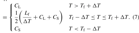
Figure 1 illustrates the relationship between the apparent heat capacityCappand the temperatureT. The shaded region
in this figure represents the latent heat, and the apparent heat capacity in the three different temperature regions is given by
Capp
¼
CL T >TfþT
1
2
Lf
T þCLþCS
Tf TTTfþT
CS T <TfT 8 > > < > > :
: ð7Þ
3.2 GLS and proposed adaptive time-step strategies In the current study, the modified LTE technique modifies the LTE estimate of the conventional GLS predictor and corrector strategy.
3.2.1 Predictor function and corrector function
As the GLS scheme, the time-step control scheme proposed in this study employs the explicit Adams-Bashforth (AB) formula as the predictor function and the implicit trapezoid rule (TR) as the corrector function. The AB formula has the form
AB:TnþP 1¼Tnþ
tn
2 2þ tn
tn1
_
T Tn
tn
tn1
_
T Tn1
: ð8Þ
As shown, the AB predictor requires two historic cooling rates, namely TT_n andTT_n1, respectively. As discussed later,
these cooling rates are obtained simply and recursively from the TR corrector results. Since TT_n1 is required, the AB
formula cannot be applied until the second time step. Error estimation therefore commences only once the second time step has been completed. The TR corrector function is formulated as
TR: Tnþ1 ¼Tnþ
tn
2 ð _
T
TnþTT_nþ1Þ: ð9Þ
Being implicit, TR can be applied directly to eq. (6) to obtain the final temperature value
CappðTinþ1Þ
2
tn
ðTinþ1TinÞ TT_in
¼ r ðkrTÞ: ð10Þ
3.2.2 LTE estimate in GLS scheme and modified LTE estimate
In the GLS scheme, the LTE estimation process commen-ces by performing Taylor series analyses of the predictor (AB) and corrector (TR) formulations given in eqs. (8) and (9), respectively. Neglecting the higher-order terms, the estimated errors between the numerical solutions and the analytical solutionsTanaðtnþ1Þat time steptnþ1are given by
AB:Tnþp 1Tanaðtnþ1Þ ¼
1 12 2þ3
tn1
tn
t3nT...n; ð11Þ
TR: Tnþ1Tanaðtnþ1Þ dðTnþ1Þ ¼
t3 n
12 T
...
n; ð12Þ
wheredðTnþ1Þis the estimated LTE of the TR solution. Since
Tnþp 1andTnþ1are available, eqs. (11) and (12) can be used to
eliminate the two unknowns,i.e.Tanaðtnþ1ÞandT
...
n, and hence
the estimated LTE of the TR solution in the GLS scheme can be obtained as
dðTnþ1Þ ¼
Tnþ1T p nþ1
3
1þtn1
tn
: ð13Þ
However, in the time-step control strategy employed in the current study, an appropriate time step is determined not on the basis ofdðTnþ1Þ, as in the conventional GLS strategy, but
from an extreme value of LTE, designated as dðTnþ1Þext,
derived on the assumption of an extreme time step text,
whose absolute value is much larger than that oftn1. From
the corrector function given in eq. (12), dðTnþ1Þext can be
written as
dðTnþ1Þext
t3ext
12 T
...
n: ð14Þ
Adopting this definition of dðTnþ1Þext, the term tn in the
denominator of eq. (13) can be replaced by text, and thus
the ratio oftn1totextapproaches zero, causing the value
of the LTE computed in eq. (13) to converge to an extreme value. Accordingly,dðTnþ1Þextcan be expressed as
dðTnþ1Þext¼
Tnþ1T p nþ1
3 : ð15Þ
The LTE can then be estimated by combining eqs. (12) and (14) to give
dðTnþ1Þ ¼dðTnþ1Þext
tn
text
3
: ð16Þ
app
C
2∆T
f
T
f
T − ∆T Tf+ ∆T
L
C
S
C
L S
f C C
L
2∆T 2
+ +
T
[image:3.595.50.290.539.596.2]In eq. (16),textis an assumptive time step which needs to
be determined. In this study,textis determined as a function
of the local temperature.
3.2.3 Novel technique for determiningtext
The Taylor series ofTT_nþ1 with forward expansion can be
written as
_
T
Tnþ1¼TT_nþTT€ntnþ
1 2T
...
ntn2þOðtn3Þ: ð17Þ
To prevent the appearance of another previous time step,i.e.
tn2, the third-order derivativeT
...
nin eq. (17) is replaced by
applying eqs. (12) and (13). As a result, eq. (17) can be written in the following semi-implicit form:
_
T
Tnþp 1¼TT_n 1þ
tn
tn1
TT_n1
tn
tn1
þ ðTnþ1T p nþ1Þ
1 1
2ðtnþtn1Þ
: ð18Þ
The first and second terms on the right hand side of eq. (18) can be replaced by eq. (8) and by assumingtn¼
text andtexttn1,textcan be expressed in terms of
the temperature and cooling rate as follows:
text¼2
Tnþ1Tn
_
T
Tnþp 1þTT_n !
: ð19Þ
Rearranging eq. (19), the temperature at the next time step can be expressed as
Tnþ1 ¼Tnþ
text
2 ð _
T TnþTT_
p
nþ1Þ: ð20Þ
Equation (20) is similar to the TR corrector function given in eq. (9) and the LTE can be approximated by eq. (14). In other words, the modified LTE given in eq. (16) can be estimated via the error comparison of two TR formulae,i.e.
eqs. (9) and (20), respectively. 3.2.4 Initialization oftext
For any given spatial node, the corresponding value of
text can be determined from eq. (19). However, if no
change occurs in the local temperature between the initial condition and the condition after the following time step(s), the denominator of this equation,i.e.the sum of the cooling rates, is equal to zero, and hence a numerical error results. Accordingly, in the proposed approach, the denominator term is assigned a small tolerance, which is sufficient to prevent a zero denominator without adversely affecting the quality of the numerical solutions.
3.2.5 Controlling the magnitude oftext
Due to its temporal singularity characteristic in space, latent heat release cannot easily be analyzed using a Taylor series approach without applying some form of correction. In the apparent heat capacity method, this singularity problem is resolved by imposing a piecewise continuity of the temper-ature drop2T(see eq. (7) and Fig. 1) as the artificial mushy zone. The latent heat release is then modeled numerically using a series of small temperature drops in2T. However, a large time step may cause the temperature drop betweenTn
andTnþ1 to exceed the value of2T, thereby violating the
piecewise continuity condition. As a result, a smaller value of the time step should be applied when modeling the phase
change phenomenon in the solidification process. In the modified LTE time-step approach used in this study, this is achieved by applying a correction totext. In the proposed
approach, rather than calculating the difference between Tn
and Tnþ1 in eq. (19), its value is artificially corrected to a
small constant valueTfclose to zero in each of the specified
time steps in order to maintain the temporal piecewise continuity state set by the apparent heat capacity method. Equation (19) becomes
text¼2
Tf
_
T
Tnþp 1þTT_n !
: ð21Þ
As a result, the value oftextspecified during the latent heat
release process is extremely small. This results in a larger value of the modified LTE computed in eq. (16) and therefore generates a smaller time step size (see Section 3.2.6). This in turn, reduces the likelihood of the time step exceeding the value of2T and ensures that nearly none of the latent heat released in the artificial mushy zone is missed in the computational procedure. Furthermore, In order to improve the nonlinear convergence, the value ofTfused in
the solution procedure of nonlinear iterations is much smaller than that used in the usual prediction process performed after a convergent temperature solution.
3.2.6 Time step selection
As in the GLS scheme, oncetexthas been determined for
each spatial node in the computational domain, the LTEs over the entire domain are used to predict the next time step size by applying the constraint that the (relative) norm of the errors at the next step should be equal to a small pre-defined value",i.e.
tnþ1¼tn "
kdðTnþ1Þk
1=3
; ð22Þ
where"corresponds to the value ofkdðTnþ2ÞkandkdðTnþ1Þk
is determined via the weighted RMS norm27)as follows:
kdðTnþ1Þk ¼
1
NT
1
T2 max
XNT
i¼1
d2iðTnþ1Þ
" #
( )1=2
: ð23Þ
Equation (22), in practice, is independent of the time step
tn since the values of tn in eq. (16) and eq. (22),
respectively, can be mutually offset during the combining process described above and thus LTE in eq. (16) becomes independent oftn.
4. Results and Discussion
This section commences by comparing the performances of the GLS, BE and proposed adaptive time step methods in solving two one-dimensional phase change problems with two different initial conditions (i.e. Ti¼Tp¼Tf and
Ti¼Tp >Tf, respectively). The performance of the three
schemes is also compared with that generated using the corresponding uniform time step methods. The feasibility of the proposed adaptive time step method is then further verified by considering the case of a two two-dimensional phase change problem.
4.1 One-dimensional phase change problem
semi-infinite area. The initial pouring temperature Tp is
assumed to be equal to or larger than the fusion temperature, Tf. When t>0, T¼Tm (mold temperature) at x¼0. The
position of the liquid-solid interface at any moment in time is indicated by s(t). For convenience, the following dimension-less variables and parameters are introduced:
¼ TTw
TfTm
; ¼tS
L2 ; X¼
x L;
S¼ s
L; C
¼Capp
CS
; and Ste¼CSðTfTmÞ
Lf ;
whereLis the characteristic length,Lf is the latent heat, and
Ste is the Stefan number representing the inverse of dimensionless latent heat. S and CS are the solid thermal
diffusivity and heat capacity, respectively. Furthermore,Tw
representsTmwhileTp ¼Tf andTf whileTp>Tf.
4.1.1 p¼f
The analytical solution for this problem was originally derived by Stefan in Ref. 31). In simulating this problem, it is assumed that x=L¼2 and X¼0:01. The mold temperature and fusion temperature thus become m¼0
and f ¼1, respectively. The total calculation time is
specified as ¼2 to ensure that ðX¼2; Þ ¼1. In addition, " is set to 0.001 in accordance with the standard GLS recommendation.27) The GLS time stepping strategy
and the proposed time stepping method both require the two initial time steps,i.e.1 and2, to be explicitly defined.
In the current simulations, both time steps are assigned a value of 0.0001. The latent heat release process, in which the temperature difference is ¼0:001 and Ste¼1, is modeled using the apparent heat capacity method. Note that because p ¼f, only a half of the artificial mushy zone
(2) is necessary in modeling the latent heat effect. For convenience, the f terms used to calculate ext
in the nþ1 selection process and the n adjustment
process are distinguished via the annotations f/sel and
f/adj, respectively and they are assigned byf/sel¼107
and f/adj¼1015, respectively. Solving this problem
[image:5.595.336.513.71.247.2]analytically, it is determined that the phase change position reaches X¼1:76at ¼2.
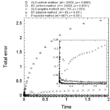
Figure 2 compares the total error histories of the GLS and BE uniform time step methods (¼0:0001) with those of the GLS, BE and proposed adaptive time step methods. Note that the error is defined here as the RMS of the total difference between the computational solution and the analytical solution over the entire domain. It is apparent that the results obtained using the proposed method are in very good agreement with those obtained using the GLS uniform time step method. Both schemes achieve a high degree of numerical accuracy. However, the number of time steps required by the proposed method (nt¼6674) is significantly lower than that required by the GLS uniform time step method (nt¼20000). In Fig. 3, it is observed that the time step size predicted by the GLS or BE adaptive time step methods increases approximately linearly over the course of the simulation. By contrast, those predicted by the proposed method oscillate strongly, albeit with a gradually increasing tendency. This phenomenon is the result of the corresponding trend in the kLTEk term resulting from the accurate latent heat release.
Figure 4 illustrates the latent heat release predictions of the GLS adaptive time step method, the BE adaptive time step method and the proposed adaptive time step method, respectively, for all of the spatial nodes over the course of Fig. 2 One-dimensional phase change problem withp¼f: total error histories of uniform time step methods, GLS and BE adaptive time step methods and proposed method.
Fig. 3 One-dimensional phase change problem withp¼f: time step size histories of uniform time step methods, GLS and BE adaptive time step methods (right scale) and proposed method.
[image:5.595.78.260.146.199.2] [image:5.595.326.526.304.457.2] [image:5.595.338.512.518.684.2]the simulation. The exact solution for the latent heat in this example is 1=Ste¼1. The total amount of latent heat released by the proposed method reaches 97.5% of the exact value at¼2because its predicted time steps are in closer agreement with the tempo of latent heat release in space. By contrast, 59.41% of the total latent heat is released by the GLS adaptive time step method and 26.37% by the BE adaptive time step method. Consequently, the GLS and BE adaptive time step methods have the faster solidification rate compared to that predicted by the proposed method, and therefore the phase change position simulated by the GLS adaptive time step method reachesX¼1:85at¼2rather thanX¼1:76, as determined analytically, and the one simu-lated by the BE adaptive time step method exceeds X¼2. The phase change position for the proposed method reaches X¼1:77, which is much closer to the analytical one. Note that in this simulation, the BE adaptive time step method takesx=L¼4corresponding to its faster solidification rate.
Furthermore, all the methods used to simulate this problem have no convergence problem encountered before the end of simulation period. The maximum number of nonlinear iterations obtained for the proposed method and GLS uniform time step method is 3, respectively. This indicates that the solution obtained by the proposed time stepping algorithm has an excellent convergence performance. This value of 3 is then taken as the minimum value ofNd for the
following one and two-dimensional simulations. Further-more, the CPU time (performed by ASUS L7300 PC with a Pentium II 600 (MHz) CPU and 196 MB RAM) for the proposed method is 19.6 sec, while for the GLS uniform time step is 69.2 sec. The result indicates that the proposed method can reach a greater numerical efficiency.
4.1.2 p> f
The analytical solution for this 1-D phase change problem was given by Carslaw and Jaeger.32) In simulating this
problem, it is assumed thatX¼3andX¼102. The mold
temperature and fusion temperature thus become m¼ 1
andf¼0, respectively. The pouring temperature is assumed
to bep¼0:3at¼0. The total simulation time is specified
as ¼0:25, which ensures that ðX¼3; Þ ¼p¼0:3.
Furthermore, when applying the proposed time-stepping method, it is assumed that "¼103. The two initial time
steps,i.e.1and2, are both assigned a value of105to
ensure convergence. The latent heat release is modeled using the apparent heat capacity method with an assumed temper-ature interval of2¼2102and Ste¼4. Furthermore,
in determining an appropriate value of ext to accurately
capture the local variations in the latent heat released during phase change, it is assumed that f/sel¼104 when
selecting the new time stepnþ1andf/adj¼1012when
adjusting the current time stepn. Note that since the latent
heat modeled by the apparent heat capacity method is associated with2and Ste, as shown in Fig. 1, the value of
f/sel must be adaptively scalable depending on the
magnitudes of2and Ste. This can be found by comparing the value off/selof the current example with that used in
the previous example. Furthermore, the value of f/adj¼
1012 is the maximum value for reaching a convergent solution. Using different values of f/ad 51012 obtains
almost identical results.
Solving the current problem analytically, it is found that the solid-liquid interface and the conduction effect reach locations ofX¼0:7 andX¼2:86, respectively, at the end of the simulation period (¼0:25). Note that the standard GLS adaptive time step method and BE adaptive and uniform time step methods are not considered in the following discussions since they have less accurate performance and are known to suffer numerical instability when applied to the current and the following two-dimensional problems using a iterative method, i.e. fully-implicit scheme (FIS). In FIS computational schemes, the apparent heat capacity is iteratively calculated according to the temperature of current time step, whereas in semi-implicit computational schemes, it is based on the temperature of previous time step and thus nonlinear iterations are not required. The results obtained using these two schemes are further analyzed in the following discussion.
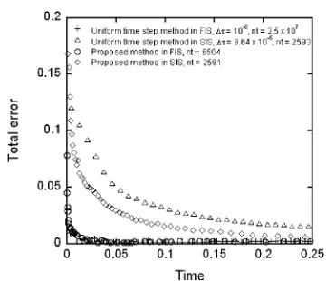
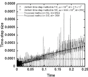
Figure 5 compares the total error history of the GLS uniform time step method with that of the proposed method for both the FIS and the SIS computational schemes. In the GLS uniform time step method implemented in the FIS scheme with ¼108, a relaxation factor (!¼0:1) is
[image:6.595.335.515.67.222.2]in both computational schemes have a gradually increasing tendency and an oscillatory type behavior due to the latent heat release.
The exact solution for the latent heat released in this case is
1=Ste¼0:25. The results presented in Fig. 7 indicate that the proposed method with the FIS scheme conserves a similar amount of latent heat during phase change as the GLS uniform time step method implemented in the FIS scheme. Due to the accurate energy balance in the process of nonlinear iterations, the total amount of released latent heat computed by the proposed method implemented in the FIS scheme is found to be 99.0% of the exact value at¼2. This value falls to 87.03% when the proposed method is implemented in the SIS scheme. By contrast, in the GLS uniform time step method, almost 100% of the total latent heat is released in the FIS scheme, while 86.39% is released in the SIS scheme.
Furthermore, the CPU time (performed by ASUS A8FM PC with an Intel Core 2 1.83 (MHz) CPU and 1024 MB RAM) for the proposed method implemented in the FIS scheme is 30.5 sec, while for the GLS uniform time step is 56990.5 sec. Within a time step, the maximum number of iteration for the proposed method is 4. These results indicate that the proposed method can reach a greater numerical efficiency.
4.2 Two-dimensional phase change problem
An infinite corner region is assumed initially to be in a liquid state at a pouring temperature Tp higher than the
melting temperature Tf. As time elapses, the boundary
temperatures along x¼0 and y¼0, respectively, are maintained at a constant mold temperatureTm that is lower
thanTf. The dimensionless analytical solution and interface
position for this 2-D phase change problem are given by Rathjen and Jiji in Ref. 33). In the dimensionless physical model, the mold, fusion and pouring temperatures are specified as m¼ 1, f¼0 and p ¼0:3, respectively.
Furthermore, the computational domain is assumed to be in the shape of a square with sides of length X¼Y ¼2. In solving the problem using the proposed method implemented in the FIS scheme, the following parameter values are assigned:X¼Y¼102,
1¼2 ¼105,"¼103,
2¼2102,
f/sel¼104 and f/adj ¼1016.
Fur-thermore, the tolerance criterion R used to evaluate the convergence condition of the temperature field is specified as
1:32106. By assigning this particular value, the average
tolerance for each point in space is 3:31011, which is
consistent with that used in the previous one-dimensional simulations of p> f. In attempting to solve the current
problem using the GLS uniform time step method, obtaining a convergent solution is difficult. As a result, the solutions obtained using the proposed method are compared with the exact results.
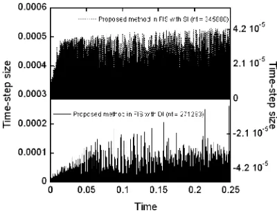
Figure 8 compares the exact solution and two simulated solutions for the phase change position (i.e. the location of the liquid-solid interface) at ¼0:25 for the case of ¼0:25, where is a non-dimensional parameter defined as Lf=½CSðTfTmÞ, i.e. the inverse of the Stefan number.
Note that DI indicates a double iterative process, while SI is a single iterative process. It can be seen that both simulated phase change interfaces are in good agreement with the exact solution. In the DI process, the line Gauss-Seidel iteration method is executed before the current nonlinear iteration method is used to compute the corresponding value ofCapp
(Note thatNdis assigned a value of 3). Conversely, in the SI
process, the two iteration methods are combined as one and Ndis assigned a value of 9,i.e.the square of that used in the
DI simulation. Fig. 6 One dimensional phase change problem with p> f: time step
histories for uniform time step method and proposed method implemented in FIS and SIS schemes.
Fig. 7 One dimensional phase change problem withp> f: latent heat release in space computed by uniform time step method and proposed method implemented in FIS and SIS schemes.
[image:7.595.344.510.68.218.2] [image:7.595.81.256.69.222.2] [image:7.595.80.255.281.430.2]Comparing the convergence performance of the two iteration schemes, a maximum of 4 nonlinear iterations are required per time step in the DI scheme, while that required in the SI scheme is 10, whose square root is less than 4. Overall, these results indicate that the proposed method has an efficient convergence performance when applied to this 2-D phase change problem. Analyzing the latent heat balances of the two simulation schemes, it is found that the DI scheme accounts for 99.49% of the exact value (0.25), while the SI scheme accounts for 99.68%. As shown in Fig. 9, this accurate latent heat balance performance results in an oscillating time-step history profile, similar to that observed in the previous simulations ofp> f.
5. Conclusions
This study has presented an adaptive time-step control scheme in which an appropriate time step is derived using a modified LTE formulation based on both extreme time step and extreme LTE values. In the approach presented in this study, the LTE-based time-step evaluation procedure is applied not only after a convergent temperature field is obtained at each time step, but also during the nonlinear iterations performed at each time step whenever a con-vergence problem is encountered. The performance of the proposed approach has been demonstrated by solving various 1-D and 2-D solidification problems using fully-implicit scheme. In general, the results have shown that the proposed approach has a high numerical accuracy (as evaluated by comparing the computed value of the total latent heat released with the exact solution), a high computational efficiency (as indicated by a low CPU time and a low total number of time steps in the simulation procedure) and a good convergence performance (as indicated by a low number of nonlinear iterations at each time step). Furthermore, it has been shown that the line Gauss-Seidel iteration method and the nonlinear iteration method used to determine an appropriate value of Capp can
be combined to create a computationally efficient and highly accurate solver for the solution of the 2-D phase change
problem. Moreover, since the time steps predicted by the proposed method are based on the local temperature, this method similarly provides a flexible reference tool for the researchers while they investigate other transient phenom-ena of a casting or solidification process, such as velocity and concentration fields.
REFERENCES
1) W. Kurz and D. J. Fisher: Fundamentals of solidification, 4th ed., (Trans Tech Publications, Switzerland, 1998) pp. 5–24.
2) W. D. Murray and F. Landis: J. Heat Transf. Trans. ASME81(1959) 106–112.
3) M. Ciment and R. B. Guenther: Appl. Anal.4(1974) 39–62. 4) M. Ciment and R. A. Sweet: J. Comput. Phys.12(1973) 513–525. 5) B. Rubinsky and E. G. Cravahlo: Int. J. Heat Mass Transf.24(1981)
1987–1989.
6) H. G. Askar: Int. J. Numer. Methods Eng.24(1987) 859–869. 7) A. J. Dalhuijsen and A. Segal: Int. J. Numer. Methods Eng.23(1986)
1807–1829.
8) D. Poirier and M. Salcudean: J. Heat Transf. Trans. ASME110(1988) 562–570.
9) V. R. Voller and C. R. Swaminathan: Int. J. Numer. Methods Eng.30 (1990) 875–898.
10) H. Hu and S. A. Argyropoulos: Model. Simul. Mater. Sci. Eng.4(1996) 371–396.
11) R. W. Lewis and K. Ravindran: Int. J. Numer. Methods Eng.47(2000) 29–59.
12) W. D. Rolph and K. J. Bathe: Int. J. Numer. Methods Eng.18(1982) 119–134.
13) Q. T. Pham: Int. J. Heat Mass Transf.28(1985) 2079–2084. 14) T. C. Tszeng, Y. T. Im and S. Kobayashi: Int. J. Mach. Tools Manufact.
29(1989) 107–120.
15) A. W. Date: Int. J. Heat Mass Transf.34(1991) 2231–2235. 16) P. H. Gaskell, P. K. Jimack, M. Sellier and H. M. Thompson: Int. J.
Numer. Methods Fluids45(2004) 1161–1186.
17) D. Kavetski, P. Binning and S. W. Sloan: Int. J. Numer. Methods Eng. 53(2002) 1301–1322.
18) D. Kavetski, P. Binning and S. W. Sloan: Adv. Water Resour.24(2001) 595–605.
19) N. Crouzet and P. J. Turinsky: Nucl. Sci. Eng.123(1996) 206–214. 20) K. Chen, M. J. Baines and P. K. Sweby: J. Comput. Phys.150(1993)
324–332.
21) J. A. Dantzig: Int. J. Numer. Methods Eng.28(1989) 1769–1785. 22) J. Douglas and T. M. Gallie: Duke Math. J.22(1955) 557–571. 23) J. S. Goodling and M. S. Khader: J. Heat Transf. Trans. ASME96
(1974) 114–115.
24) R. S. Gupta and D. Kumar: Comput. Meth. Appl. Mech. Eng.23(1980) 101–109.
25) R. S. Gupta and D. Kumar: Int. J. Heat Mass Transf. 24 (1981) 251–259.
26) T. Ouyang and K. K. Tamma: Int. J. Num. Meth. Heat Fluid Flow6 (1996) 37–50.
27) P. M. Gresho, R. L. Lee and R. L. Sani: Recent Advance in Numerical Methods in Fluids, (Pineridge Press, Swansea, 1980) pp. 36–38. 28) FIDAP 8 Theory Manual, (Fluent Inc, New Hampshire, 1998) pp. 7.36–
38.
29) H. C. Peng and L. S. Chao: Proc. The Seventh International Congress on Thermal Stresses, ed. by C. K. Chao and C. Y. Lin, (National Taiwan University of Science and Technology, 2007) pp. 619–622. 30) W. F. Ames:Numerical Methods for Partial Differential Equations,
2nd ed., (Academic Press, New York, 1977) pp. 144–147. 31) J. Stefan: Ann. Phys. U. Chem.42(1891) 269–286.
32) H. S. Carslaw and J. C. Jaeger:Conduction of Heat in Solids, 2nd ed., (Oxford University Press, Oxford, 1959) pp. 283–286.
33) K. A. Rathjen and L. M. Jiji: J. Heat Transf. Trans. ASME93(1971) 101–109.
[image:8.595.68.268.71.225.2]