Local time stepping with adaptive time step control for a two-phase fluid system

F. Coquel, Y. Maday, S. M¨uller, M. Postel and Q. H. Tran, Editors

LOCAL TIME STEPPING WITH ADAPTIVE TIME STEP CONTROL FOR A

TWO-PHASE FLUID SYSTEM

Fr´

ed´

eric Coquel

, Quang Long Nguyen

, Marie Postel

and Quang Huy

Tran

R´esum´e. Cet article aborde la question de l’utilisation efficace des maillages adaptatifs en vue de simuler correctement le transport des fronts sur des temps longs avec un coˆut CPU raisonnable. Ces singularit´es proviennent des syst`emes de lois de conservation mod´elisant les ´ecoulements diphasiques `

a travers les conduites p´etroli`eres. Nous proposons non seulement un cadre multir´esolution afin d’ajuster le pas d’espace `a la r´egularit´e locale de la solution, mais aussi une strat´egie de pas de temps local afin d’all´eger les contraintes dues `a la condition CFL de stabilit´e. Nous examinerons plus particuli`erement le choix optimal des micro pas de temps `a l’int´erieur d’un macro pas de temps. Nous pr´esentons les simulations num´eriques pour illustrer l’efficacit´e des m´ethodes pr´econis´ees.

Abstract. This paper is concerned with how to make effective use of adaptive grids to correctly simulate the transportation of fronts over a long range of time under reasonable CPU time. These step gradients arise from systems of conservation laws modelling two-phase flows in pipelines. We propose not only a multi-resolution setup in order to adapt the space grid to the local smoothness of the solution, but also a local time stepping strategy in order to alleviate the constraints due to the CFL stability condition. A special focus is given to the optimal choice of micro time steps within a macro time step. Numerical simulations are presented to illustrate the efficiency of the methods put forward.

Introduction

We are interested in accurate and fast computation of two-phase flows in pipelines within the context of a drift-flux model given to us by physicists. This one-dimensional model consists of nonlinear conservation laws involving very expensive algebraic closure laws coming from experimental data. The closure laws are so intricate that they can even spoil the hyperbolicity of the PDE system. Whenever hyperbolic, this model contains two types of waves, namely, fast acoustic waves and slow kinematic waves. Only slow kinematic waves are interesting to the oil field engineers.

This setup is a good candidate for adaptive methods such as those introduced by Harten [15] and Co-hen et al [6]. In analyzing the local smoothness of the solution using a wavelet-like transformation, we manage to design a local refinement strategy for adapting the mesh-size and for moving the mesh along with the solution. By “moving the mesh,” we mean that the fronts propagating at slow kinematic speeds

∗_{This work was supported by the Minist`ere de la Recherche under grant ERT-20052274:Simulation avanc´ee du transport}

des hydrocarburesand by the IFP.

1

UPMC Univ Paris 06, UMR 7598 LJLL, Paris, F-75005 France

2

CNRS, UMR 7598 LJLL, Paris, F-75005 France

3

IFP, D´epartement Math´ematiques Appliqu´ees, 1 et 4 avenue de Bois-Pr´eau, 92852 Rueil-Malmaison, France c

EDP Sciences, SMAI 2009

are suitably captured by refined cells and accurately computed. Comprehensive description and analysis of multi-resolution techniques can be found in [5] and [18]. The successful use of this type of methods for our problem was demonstrated in [1, 10].

Although multi-resolution has brought us significant speed-up factors, e.g., about 3 for a typical run, we are still hampered by the fact that the time step is the same all over the grid and therefore must be governed by a CFL condition on the smallest mesh-size. The goal of this paper is to overcome this restriction with the help of local time stepping techniques. By using different time steps in different areas of the grid, we legitimately hope to further enhance the computational performance of the code, since there will be much less calls to the expensive algebraic closure laws. Early works in this direction go back to Bergeret al[4], Osheret al[22] and more recent works like [23], [3] and [12] provide alternatives to the method adopted in the present paper. Seemingly a natural enhancement to a space adaptive scheme, the actual implementation of a Local Time Stepping strategy (LTS) is usually not straightforward. In fact, the additional book-keeping infered by the synchronization of the solution on the different discretized time grids might act as a deterrent, if the data structure is not clever enough to lead to interesting gains in computing time. Another inconvenience is the lack of analysis for such methods in the context of hyperbolic PDEs, whereas some stability results are available for parabolic equations [11, 14].

Recently a local time stepping strategy in the context of the fully adaptive scheme described in the

previous paragraph has been proposed in M¨uller et al[20], and successfully implemented for various PDE

systems in several dimensions [12,17,19]. This method was adapted in the context of the Lagrange-projection semi-implicit scheme for a simplified version (no-slip law) of our diphasic model in [8, 9]. We now carry it over to the full model in the explicit setting. The novelty on which we wish to lay emphasis is the optimal choice of the micro time steps within a macro time step.

This paper is organized into two parts. We first recall the model and the basic numerical scheme before any adaptive treatment. Then, we show how to formalize the multi-resolution and local time stepping philosophy to the problem at hand. Finally, some numerical results are supplied.

1.

_{Physical model and numerical scheme}

1.1.

Physical model in Eulerian coordinates

Over the state space

Ωw={w= (ρ, ρv, ρY) T _∈

R3|ρ >0, Y ∈[0,1]}, (1)

we consider the problem of finding a functionw:R+×R→Ωw such thatw(t, x) solves

∂t(ρ) +∂x(ρv) = 0 (2a)

∂t(ρv) +∂x(ρv2+P) = s (2b)

∂t(ρY) +∂x(ρY v+σ) = 0. (2c)

In (2), ρ is the density of the two-phase mixture, v is the velocity and Y is the gas mass-fraction. The

quantitiesP =P(w),σ=σ(w) ands=s(w) are given by

σ = ρY(1−Y)φ (3a)

P = ρY(1−Y)φ2+p (3b)

s = −ρgsinθ−1

2Cρv|v| (3c)

System (2), referred to as the Drift-Flux Model(DFM), expresses the conservation laws associated with the mixture density, the total momentum and the gas density. It can be put under the abstract form

∂tw+∂xf(w) =s(w), (4)

using the vector notations

f(w) =wv+g(w) (5a)

g(w) = (0, P(w), σ(w))T (5b)

s(w) = (0, s(w),0)T_{. (5c)}

Except for a few specific instances of the closure laws p and σ, nothing can be said in general about the

hyperbolicityof (2). Forσ≡0, most notably, the DFM model (2) degenerates to the standard Euler model.

The latter is known to be strictly hyperbolic provided that

∂ρp(ρ, Y)_Y >0. (6)

By analogy with this case, we require that

∂ρP(w)Y,v>0, (7)

with a little abuse of notations regarding the arguments ofP. When strict hyperbolicity occurs, it is usually observed that the three real eigenvalues

λ−(w)< λ0(w)< λ+(w), (8)

of the Jacobian matrix∇wf(w) satisfy

|λ0(w)| ≪ |λ−(w)| ≈ |λ+(w)|. (9) In other words, there are two scales of wave velocities with distinctive orders of magnitude: the fast acoustic waveλ± and the slow kinematic waveλ0. To put (9) differently, the flow regime that most often prevails in the context of oil transportation corresponds to low Mach numbers.

1.2.

Physical model in Arbitrary Lagrange-Euler coordinates

It is judicious to separate fast and slow waves in order to make positivity properties easier to be guaranteed. The full details of this approach can be found in [7]. Here, we simply give the core ideas.

We introduce a new referential frame, in which the coordinates are denoted byχ. This frame is neither

the material (Lagrangian) configuration nor the laboratory (Eulerian) configurationx. Instead, it moves at the imposed speedv−wwith respect to the laboratory. Letx=x(χ, t) be the correspondence between the moving frame and the laboratory frame, and define

J=∂χx_t (10)

to be the dilatation rate. Then, it can be proven [13, 16] that system (4) is equivalent to

∂t(J) +∂χ(w) −∂χ(v) = 0 (11a)

The above form highlights the role of the arbitrary velocityw, thanks to which we can now apply a splitting technique.

Let ∆t >0 denote the time step. Each iteration from timetn _{to t}n+1_=tn_{+ ∆tis made up of two steps}

n→n♯→n+ 1. (12)

(1) The Lagrange step. Starting fromJn_{= 1, we solve}

∂t(J) −∂χ(v) = 0 (13a)

∂t(wJ) +∂χ(g(w)) = Js(w). (13b)

Writing out all components, the above system reads

∂t(J) −∂χ(v) = 0 (14a)

∂t(ρJ) = 0 (14b)

∂t(ρvJ) +∂χ(P) = Js (14c)

∂t(ρY J) +∂χ(σ) = 0. (14d)

By doing so, we have temporarily disregarded the convection due tow. However, as was the case for the initial system (4), no claim can be made about the hyperbolicity of the Lagrangian system (13). On the other hand, the difficulties associated with the closure laws remain identical.

In a series of previous works [1, 2, 10], it has been demonstrated thatrelaxation can be a handy tool to help us solve (13). In essence, relaxation amounts to replacing (14) by

∂t(J) −∂χ(v) = 0 (15a)

∂t(ρJ) = 0 (15b)

∂t(ρvJ) +∂χ(Π) = Js (15c)

∂t(ρΠJ) +∂χ(a2v) = 0 (15d)

∂t(ρY J) +∂χ(Σ) = 0 (15e)

∂t(ρΣJ) +∂χ(b2Y) = 0, (15f)

in which Π,Σ are the auxiliary variables representing P(w) and σ(w), while a, b are two positive

parameters. For stability reasons,aandb must be subject to the Whitham conditions

a >

r

−∂τP(u)_v,Y +

∂vP(u)_τ,Y

2

(16a)

b >∂Yσ(u)τ,v

, (16b)

where

u= (τ:=ρ−1, v, Y). (17)

The interest of (15) lies in the fact that it is always hyperbolic. Indeed, its characteristic speeds are

−aτ, −bτ, 0, 0, bτ, aτ. (18)

(2) The projection step. Starting from the intermediate staten♯, we setw=v and solve

∂t(J) +∂χ(v) = 0 (19a)

By doing so, we recover the motion of the particles. Choosing w=uyields Jn+1_{= 1 at the end of} the step, and the mesh returns to its initial configuration. Multiplying (19a) byw and substracting to (19b), we end up with

∂tw+v

J∂xw= 0. (20)

Since all components of w are transported at the same characteristic speed v/J, this step is also

called theremapstep.

1.3.

Numerical scheme

The two steps need to be fully explicited at the discrete level. We decompose the space domain into cells labeled by subscriptsj∈Z. The edges of the cells are designated by subscriptsj+ 1/2, while the size of cell j is ∆xj.

(1) The Lagrange step. Taking as granted thatJn

j = 1, we discretize (13) by

Jjn♯−Jjn

∆t −

e

vn

j+1/2−ev

n j−1/2

∆xj = 0 (21a)

(wJ)n♯j −(wJ)nj

∆t +

e

gn_j+1/2−_eg_jn_−1/2

∆xj = (J

s)nj, (21b)

with the notation

e

gn_j+1/2= (0,σenj+1/2,Pejn+1/2)T. (22) The flux values are retrieved by solving the Riemann problem associated with the relaxation system (15) at edgej+ 1/2. This results in

e

vnj+1/2 = ev(wnj,wnj+1) = vn

j +vnj+1

2 −

Pn j+1−Pjn

2aj+1/2

(23a)

e

Pjn+1/2 =Pe(wnj,wnj+1) = Pn

j +Pjn+1

2 −aj+1/2

vn j+1−vjn

2 (23b)

e

σnj+1/2 =eσ(wnj,wnj+1) = σn

j +σnj+1

2 −bj+1/2

Yn j+1−Yjn

2 , (23c)

where the positive parametersaj+1/2, bj+1/2 are subject to the discrete Whitham conditions

aj+1/2>max{

q

−Pτ(unj) + (Pv(unj))2,

q

−Pτ(unj+1) + (Pv(unj+1))2 (24a)

bj+1/2>max{|σY(unj)|,|σY(unj+1)|}. (24b)

Note that we have used the relaxation system (15) only as a virtual tool in order to derive the flux values (23). In reality, the additional terms Π and Σ are not computed by (15) but simply reset by Πn♯_j =P(wn♯_j ) and Σn♯_j =σ(wn♯_j ).

(2) The projection step. Taking as granted thatw=ev, we discretize (19) by Jjn+1−J

n♯ j

∆t +

e

vn

j+1/2−evjn−1/2

∆xj = 0 (25a)

(wJ)n_j+1−(wJ)n♯_j

∆t +

(w_ev)n♯_j+1/2−(w_ev)n♯_j−1/2 ∆xj

with the upwind flux

(w_ev)n♯_j+1/2=wn♯_j (_evj+1/2)++wn♯j+1(evj+1/2)−. (26) The velocity to be prescribed at the edges for the projection step is an outcome of the Lagrange step.

To see how the overall scheme combining both steps gives rise to a consistent approximation of the initial model (2), let us add (13) and (19). We obtain

J_jn+1−Jn j

∆t = 0 (27a)

(wJ)nj+1−(wJ)nj

∆t +

ef_jn♯_+1/2−ef_jn♯_−1/2

∆xj = (J

s)nj, (27b)

where

ef_jn♯_+1/2=wn♯_j (_evn

j+1/2)++w

n♯

j+1(evnj+1/2)−+egnj+1/2. (28) SinceJn

j = 1, we haveJjn+1= 1 and the resulting scheme

wn_j+1−wn_j

∆t +

ef_jn♯_+1/2−ef_jn♯_−1/2

∆xj

=snj (29)

clearly appears to be a discretization of the Drift-Flux Model via a consistent fluxef_jn♯_+1/2. This flux is about the only thing that will be passed to the multi-resolution and local time stepping subroutines.

1.4.

CFL conditions and positivity properties

Besides the Whitham conditions (24), we impose various other CFL conditions to ensure stability. (1) Since the non-zero characteristic speeds of the Lagrangian step are±aτ and±bτ, we require

aj±1/2∆t ρn

j∆xj <

1

2 (30a)

bj±1/2∆t ρn

j∆xj <

1

2. (30b)

In practice,b≪a(which is a consequence of|λ0| ≪ |λ±|). Therefore, it is expected that only (30a) needs to be met.

(2) Since the characteristic speed of the projection step isw=v_e, we require

|evn j±1/2|∆t

∆xj

<1

2. (31)

The edge velocities _evn

j+1/2 are computable before updating the variables. Again, it is observed for most test cases in the low Mach regime that

|_evn

j±1/2| ≪aj±1/2τjn. (32)

From (31), we infer that

ρn♯j >0. (33)

Indeed,ρn♯j = (τn♯)−1and

τ_jn♯=τn j −

∆t ρn

j∆xj

(_evn

j+1/2−evjn−1/2) (34a)

=τjn

1−ev

n j+1/2∆t

∆xj

+ev

n j−1/2∆t

∆xj

(34b)

> τjn

1−|ev

n j+1/2|∆t

∆xj

−|ve n j−1/2|∆t

∆xj

. (34c)

The last right-hand side is obviously positive under (31). Furthermore, we have

ρnj+1>0. (35)

Indeed, multiplying (25a) bywn♯_j and subtracting the product to (25b), we end up with

wn_j+1=wn♯_j − ∆t

∆xj (ev n

j−1/2)+(w

n♯ j −w

n♯

j−1) + (evjn+1/2)−(w

n♯ j+1−w

n♯ j ) (36a) =

1−(ev n

j−1/2)+∆t ∆xj

+(ev

n

j+1/2)−∆t ∆xj

wn♯_j +(ev

n

j−1/2)+∆t ∆xj

wn♯_j−1−(ev n

j+1/2)−∆t ∆xj

wn♯_j+1. (36b)

But

1−(ev n

j−1/2)+∆t ∆xj

+(ev

n

j+1/2)−∆t ∆xj

≥1−|ev n j−1/2|∆t

∆xj

−|ev n j+1/2|∆t

∆xj

>0. (37)

This implies that (36b) is a convex combination. Looking at the first component, this means that ρn_j+1 is a convex combination ofρn♯_j−1,ρn♯_j and ρn♯_j+1, all of which are positive by (33). By a similar (but lengthier) technique, we are in a position to establish that

Y_jn+1∈[0,1]. (38)

2.

_{Fully Adaptive Multiresolution scheme}

We start this section with a brief description of the space adaptive scheme designed in [6]. We refer to [10] and [1] for details and numerical examples in the context of diphasic flows. A more thorough study of the adaptive method for the Lagrange projection formulation of the simplified model (without drift) is proposed in [8]. In the second paragraph we describe how we adapt the local time stepping strategy proposed by [20] to our problem where the duration of the local time step is controlled by the solution.

2.1.

Space adaptivity

We consider a uniform mesh with step size ∆x0, whose cells are denoted by Ω0,j. Starting from this coarsest

discretization labeled 0 we define a hierarchy of K+ 1 nested grids (Sk)k=0,...,K by dyadic refinement, with

cells Ωk,j = Ωk+1,2j∪Ωk+1,2j+1 of size ∆xk= 2−k∆x0.

Initially, the piecewise constant vector-valued functionwis defined on the finest grid where it is represented by the sequence of its mean valueswK = (wK,j)j on the cells ΩK,j. The coarsening or projection operator

Pk

k+1consists in cell averaging from one grid to the coarser one. The inverse operatorPkk+1predicts the mean

operator enjoys several useful properties. It is local, its stencil width is 2s+ 1. It is exact for polynomials of degree lower or equal to 2s. By construction it preserves the mean values, i.e. Pk

k+1Pkk+1 =Id. Thanks

to this consistency property the difference between the exact and predicted values on two subdivisions of a coarse cell are symmetric. We define the detail vectordk+1 as the value of this differencewk+1−P_kk+1wk on the left-hand side subdivisions on levelk+ 1.

The two vectors wk+1 and (wk,dk+1) are of same length and we can usedk+1 along with wk and the

prediction operator P_kk+1 to recover wk+1 entirely. Iterating this encoding operation from the finest level down to the coarsest provides the multiscale representation m = (d0,d1, . . . ,dK) = MwK, where the notation has been extended tod0=w0. The indices of the multiscale representationmvary in

∇K ={[0, . . . , N0],[0, . . . , N0], . . . ,[0, . . . ,2K−1N0]}.

Thanks to the polynomial exactness of the prediction operatorP_kk+1, a small detail in absolute value means that the solution can be locally approached by a polynomial, quadratic in our case (s= 1). We can use this property to design a grid where the size of the mesh varies and is adapted to the local smoothness of the solution. Given level-dependent threshold values ε= (εk)k=0,...,K, we introduce the subset of ∇K

Γε= Γ(ε0,· · · , εK) :={γs.t.|dγ| ≥ε|γ|}, where |γ|=|(k, j)|=k. (39)

For practical purposes it is necessary to enlarge this set of significant details into a gradual tree, which is defined recursively by

(i, k)∈Γ→

i 2

+l, k−1

∈Γ, |l| ≤g.

Choosing the grading parameter g = 1 ensures that the stencil of the prediction operator P_kk+1 always

belongs to the tree. We can then define an adaptive grid Sε where the local size of the cell will be the grid

step corresponding to the finest non negligible detail

Sε=(k, j), k∈ {0, . . . , K}, j∈ {0, . . . ,2kN0}, s.t. (k,⌊j/2⌋)∈Γε

and (k+ 1, j)∈/Γε , (40)

where ⌊j⌋ denotes the integer part of j. The reverse decoding operator M−1 _{is then partially applied to} obtain a discretized representation on the adaptive gridSε. The idea is to apply the finite volume scheme

(29) discretizing the evolution operator on this object. Relying on the hyperbolicity of the system of PDEs, it is possible to predict the propagation of the fronts which move at finite speed, and also their formation to design a grid suitable to represent the solution at two consecutive times steps tn _{and t}n+1 _{— that is} satisfying the thresholding condition (39). The prediction of the refined treeeΓn+1

ε is actually the bottleneck

of the method. In practice we use the heuristic rules of Harten [15] and the complete adaptive algorithm goes as follows:

Algorithm 1Adaptive algorithm

Initialization: encoding of the initial solution usingPk

k+1 and definition of Γ0ε using (39). fortime stepn= 0, . . . , N−1 do

Prediction ofeΓn+1

ε ⊃Γnε ∪Γnε+1 .

Partial decoding ofwε,n_onSen+1

ε usingPkk+1 on (40).

Evolution ofwε,nto wε,n+1 on the adaptive gridSen+1 _{by applying (29).} Partial encoding ofwε,n+1using Pk

k+1 and definition of Γnε+1 using (39)wε,n+1and thresholding. end for

In this adaptive algorithm the time step ∆t appearing in the evolution scheme (29) is controlled by stability conditions and to emphasize its dependency on the solution we now denote it as

∆tn≤ min

(k,j)∈Sen+1

ε

1 2

∆xk |_evn

k,j±1/2| ,∆xkρ

n k,j

ak,j±1/2

!

, (41)

whereevn

k,j±1/2 is the speed at the interface computed by (23a) andak,j±1/2satisfies the Whitham condition (24). The time step ∆tn _{is set globally for the whole mesh. It therefore depends on the size of the smallest}

cell belonging toSen+1

ε . In practical applications using a hierarchy ofK grids, the ratio between the largest

and smallest cells is 2K_{. This means that in the smooth areas of the domain where the solution is discretized}

on coarsest cells it is updated with a time step 2K _{times smaller than the limit set locally by the stability}

conditions (30,31). This obviously infers a loss in computing efficiency. In the next section, we describe how to implement a local time stepping strategy to use a spatially varying time step that is locally adapted to the size of the cell.

2.2.

Local time stepping and time step control

In our case the multiresolution scheme is based on a hierarchy of nested dyadic grids. The major ingredient of a Local Time Stepping (LTS) method is therefore the design of a macro time step, suitable for the coarsest level cells, along with a cascade of intermediate time steps at which the solution defined on finer levels is updated in turns.

There are three important issues to consider in the design of such an algorithm:

(1) Control and update the length of the local time step so that the stability condition (41) is locally satisfied.

(2) Ensure the synchronization of the solution in a conservative way at interfaces between cells of different size.

(3) Perform partial regriding at intermediate time steps in order to minimize the predicted refinement of the adaptive grid.

The first point is motivated by the first section, where a lot of effort has been spent in the design of a stability condition on the time step ensuring natural physical bounds of the density and the gas mass fraction. We will illustrate in the numerical simulations in the next section that it is important to make the intermediate time steps variable and dependent on the solution evolution. The way we propose to do this is based on a generalization of the algorithm proposed in [20], which assumes a dyadic subdivision of the macro time step to be used on the coarsest level. The two other points are treated in [20] and we will briefly rephrase them in the context of our variable time step implementation.

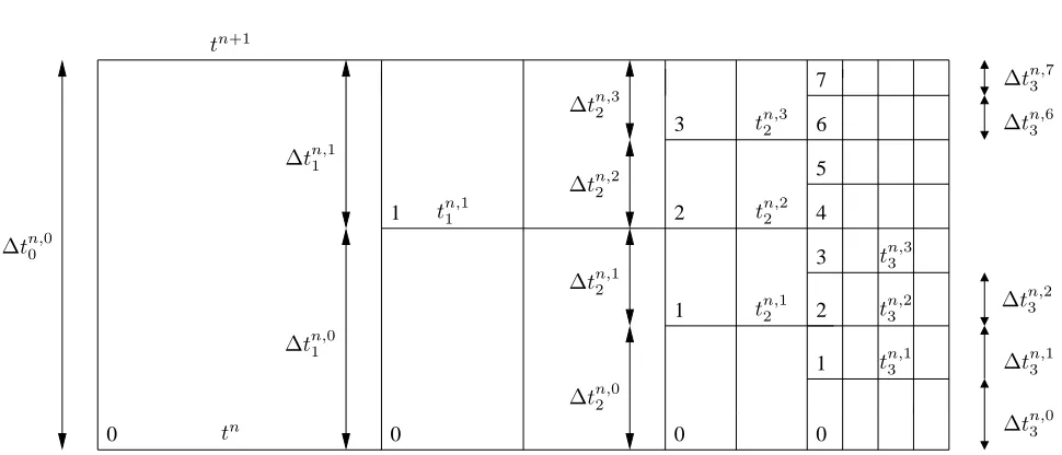
The Figure 1 illustrates the macro time step subdivision in the case of a four-level hierarchy. In the general case, the macro time step ∆tn=tn+1−tn is subdivided in a hierarchical way mimicking the spatial dyadic subdivision. Starting from ∆tn _{= ∆t}n,0

0 , the time steps to be used at the different levels are defined by

recursive subdivision

∆tn,ik = ∆t n,2i k+1+ ∆t

n,2i+1

k+1 . (42)

The intermediate time steps ∆tn,i_k will be used to update the cells active at levelkat the intermediate times tn,i_k

tn,i_k +1=tn,i_k + ∆t_kn,i, fori= 0, . . . ,2k−1,

with the convention

tn =tn,k0 andtn+1=t n+1,2k

0 0 1 0 1 2 3 0 1 2 3 4 5 6 7

∆tn,00

∆tn,10 ∆tn,₁1

∆tn,₂0 ∆tn,₂1 ∆tn,₂2 ∆tn,23

∆tn,₃0 ∆tn,31 ∆tn,₃2 ∆tn,36 ∆tn,37

tn,31 tn,32 tn,33

tn,21 tn,22 tn,23

tn,11

tn

tn+1

Figure 1. A four-level adaptive grid, with the level dependent intermediate time step numbering

Note here that not all levels are concerned by the updating process at a given intermediate time tn,i_K . To make this precise, we define at each intermediate stepi= 1, . . . ,2K _{a synchronization levelk}

i

ki:= min{k, 0≤k≤K, i mod 2K−k= 0}. (43)

It indicates the coarsest level above which cells are synchronized at intermediate timetn,i_K . The cells at level k, withki≤k≤Kare updated from their previous state at timetn,q_k using the appropriate time step ∆tn,q_k

with

q(i, k) =

i−1 2K−k

.

We now address the actual evaluation of the micro time step ∆tn,iK fori= 1, . . . ,2K which must vary in

time, that is within the macro time step, so that the bound (41) is satisfied by all intermediate times steps ∆tn,i_k fori= 1, . . . ,2k_.

We denote byFn,i the set of indices of cells where fluxes must be updated before synchronization of the solution at the intermediate time tn,i_K

Fn,i=n(k, j)∈Seεn+1, fork≥ki−1

o

.

Then the first micro time step is bounded by

∆tn,_K0≤∆xK min

(k,j)∈Fn,0

0≤k≤K

min 1

2 1

|_evn k,j±1/2|

, ρ

n k,j

ak,j±1/2

!

(44)

and the subsequent micro time steps are designed to be non increasing

∆tn,i_K = min

∆tn,i_K−1,∆xK min

(k,j)∈Fn,i

0≤k≤K

min

1 2

1

|_evn k,j±1/2|

, ρ

n k,j

ak,j±1/2

The intermediate time steps ∆tn,ik are then built up adaptively by summing the micro time steps with the

recursion (42). With these notations we illustrate the synchronization method on an example in the case of

wn_k,j−2 fn

k,j−2

wn_k,j−1

fn k+1,2j−1

f_kn,₊₁1_,2j−1

wn_k,j+1₋₁ wn_k+1+1_,2j

wn,_k+11_,2j

wn_k+1,2j wn,_k,j1₋₁

∆tn,_k+10 ∆tn,_k+11

tn,k0

tn,k1

tn,_k+11

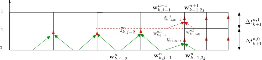
Figure 2. Local Time Step method for two refinement levels. The solution discretized on

levelk+ 1 is updated in twomicro_{time steps. The solution discretized on levelkis updated} in a singlemacro _{time step everywhere except in the transition zone (here of width 2).}

a two-level hierarchy represented in Figure 2. The little arrows on the vertical lines indicate which fluxes

must be computed. The part of the solution discretized on the fine level (numberedk+ 1) is first updated

fromwn_k+1,2j town,_k+11_,2j using the micro time step ∆tn,_k+10 . The data necessary to compute the fluxf_kn,₊₁1_,2j−1

must be synchronized at timetn,_k+11 . The neighbor cells (k, j−1) and (k, j−2) on the left of the cell 2j must therefore also be updated at the intermediate time tn,k+11 even though they belong to the coarser levelk.

The intermediate valuesw_k,jn,1₋₁ andw_k,jn,1₋₂are then used along withw_kn,₊₁1_,2j andw_kn,₊₁1_,2j+1 to compute the fluxf_kn,₊₁1_,2j−1.

The fluxes f_k,jn ₋₂ and f_k,jn ₋₁ remain valid for the macro time step at the interface of cells (k, j−2) and (k, j−1) and are used one more time to updatew_k,jn,1₋₂ andw_k,jn,1₋₁to their final valuew_k,jn+1₋₂ andwn_k,j+1₋₁.

This is formalized by designing for each level k= 0, . . . , K−1 a transition zoneC¯k _{containing the cells}

on levelkwhich belong to the stencil of the evolution scheme (29) of cells on levelk+ 1.

Note that this scheme is consistent but induces an additionalO(∆t2_{) error, except for first order two-point} stencil fluxes. The costly part in the algorithm is the flux evaluation itself, since the update of the solution in the form (29) consists in algebraic operations. A simpler way of implementing the LTS algorithm, suggested in [19], consists therefore in updating all the cells at each intermediate time step using the last computed flux value, and not only the cells belonging to the transition zone. The extra computations done in updating the coarse cells at each intermediate time instead of a single time step should be balanced by the economy in book-keeping provided by this simplification. Our implementation is based on the original strategy proposed in [20] where the cells outside transition zones are updated only when needed with the time step adapted to their size.

Algorithm 2Local Time Stepping inner loop at timetn forintermediate time steptn,i_K ,i= 1, . . . ,2K _do

Update fluxes on cells that have been updated attn,i_K−1. Compute ∆tn,q_k (i,k)fork=Kցki.

forlevelsk=Kցki do

w_k,jn,i=wn,q_k,j(i,k+1)−∆t n,q(i,k+1)

k+1

∆xk

f_k,jn,q₊₁(i,k_/+1)₂ −f_k,jn,q₋(i,k_1/2+1) if (k, j)∈C¯k w_k,jn,i=wn,q_k,j(i,k)−∆t

n,q(i,k)

k

∆xk

f_k,jn,q₊₁(i,k_/)₂−f_k,jn,q₋(i,k_1/)₂ otherwise

end for

for(k, i)∈C¯ki−1 do w_k,jn,i=wn,q_k,j(i,k+1)−∆t

n,q(i,k+1)

k+1

∆xk

f_k,jn,q₊₁(i,k_/+1)₂ −f_k,jn,q₋(i,k_1/2+1) end for

end for

The important point in this algorithm is the direction of the inner loop on the discretization levels to perform the solution update. The solution on the coarser levels is updated last, and this makes it possible to compute the corresponding time step so that it adds up to the sum of its intermediate time subdivisions. This adaptive building up of the macro time step is made possible by the synchronization method original to the chosen approach. Other LTS schemes are based on predictor corrector methods like the one proposed by Osheret al[22] or by Domingueset al[11] in the context of multiple stages Runge-Kutta schemes. In these approaches the solution in the transition zones on level k is updated first to its own synchronization time (that would bewn_k,j+1₋₁andwn_k,j+1₋₂in our two-level example) , and the data needed to update the solution on levelk+ 1 is interpolated at timetn,_k+11 (w_k,jn,1₋₁andwn,_k,j1₋₂). These strategies require to know the complete time step decomposition of the macro time step before starting to update the solution.

It is easy to check from the definition (43) or by looking at the time-space hierarchy displayed in Figure 1 thatki=Kwheniis odd. The partial regriding mentioned at the beginning of the paragraph is therefore

performed only after even time steps on levels betweenki+ 1 andK.

3.

_{Numerical simulations}

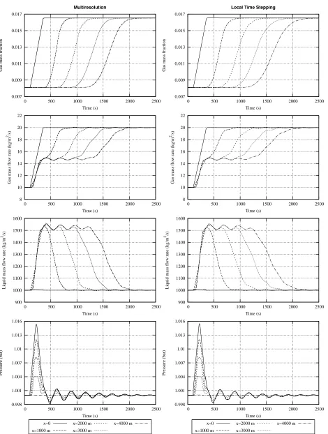
We illustrate the numerical method designed in the previous paragraph on a realistic test case modeling a 4km long pipeline. A constant flow mixture of gas and oil is injected at the inlet for 100s. Then the gas flow increases linearly for 100s from 10kg/m2_{/s to 20kg/m}2_{. After t= 200s it is kept constant until the end of} simulation which lasts 2500s. The oil flow is kept constant equal to 1000kg/m2_{/s throughout the simulation.} The pressure at the outlet of the pipe is also kept constant equal to 10 bars. We use the thermodynamical and hydrodynamical closure laws (incompressible liquid and Zuber-Findlay) described in [21]. We compare the numerical solutions obtained using the standard global time multiresolution and the local time stepping

scheme, on a 5-level hierarchy starting with 256 cells on the finest level (∆x =15.625m). The threshold

0.998 1.001 1.004 1.007 1.01 1.013 1.016

0 500 1000 1500 2000 2500

Pressure (bar) Time (s) x=0 x=1000 m x=2000 m x=3000 m x=4000 m 0.998 1.001 1.004 1.007 1.01 1.013 1.016

0 500 1000 1500 2000 2500

Pressure (bar) Time (s) x=0 x=1000 m x=2000 m x=3000 m x=4000 m 900 1000 1100 1200 1300 1400 1500 1600

0 500 1000 1500 2000 2500

Liquid mass flow rate (kg/m

2/s) Time (s) 900 1000 1100 1200 1300 1400 1500 1600

0 500 1000 1500 2000 2500

Liquid mass flow rate (kg/m

2/s) Time (s) 8 10 12 14 16 18 20 22

0 500 1000 1500 2000 2500

Gas mass flow rate (kg/m

2/s) Time (s) 8 10 12 14 16 18 20 22

0 500 1000 1500 2000 2500

Gas mass flow rate (kg/m

2/s) Time (s) 0.007 0.009 0.011 0.013 0.015 0.017

0 500 1000 1500 2000 2500

Gas mass fraction

Time (s) Multiresolution 0.007 0.009 0.011 0.013 0.015 0.017

0 500 1000 1500 2000 2500

Gas mass fraction

Time (s)

Local Time Stepping

Figure 3. Time variations of the gas mass fraction, flow rates and pressure at five

mea-surement points in the pipeline. Multiresolution (left) and Local Time Stepping (right). Explicit 1st order scheme, 256 cells, 5 levels,ε= 10−3

3.1.

Time step evolution

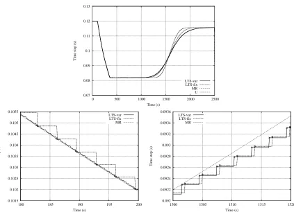
Due to the strong nonlinearity of the model and its coupled vector structure there are no invariant regions in the phase space of the solution. It is therefore impossible to predict a time step from the initial condition which would remain suitable throughout the computation. Actually, in the chosen test case, the stiff changes in input flow at the inlet of the pipe transmits itself to the flow inside the pipe and induces changes in the stability condition on the time step. The evolution of the time step monitored by the stability condition is displayed in Figure 4. It exhibits a region where it decreases, corresponding to the increase in gas input. Towards the end of the computation it starts to increase gently. We take a closer look at the evolution of the time step in those two regions. In the decreasing region between 180s and 200s, thanks to the control on the micro time step, the time step of both adaptive schemes stays close to the time step of the uniform scheme. For sake of comparison we also display the time step evolution if the micro time step is kept constant during each macro time step. This would obviously lead to violate the stability condition. In the other region of interest — after 1200s — the time step monitored by the stability condition increases gently in the uniform and global time stepping multiresolution case. The micro-time step is forbidden to increase during a macro time step and this leads to a gentler increase than in the uniform case. Yet the LTS scheme time step eventually catches up with the uniform evolution which further corroborates the robustness of our time stepping strategy.

0.07 0.08 0.09 0.1 0.11 0.12 0.13

0 500 1000 1500 2000 2500

Time step (s)

Time (s)

LTS-var LTS-fix MR U

0.1015 0.102 0.1025 0.103 0.1035 0.104 0.1045 0.105 0.1055

180 185 190 195 200

Time step (s)

Time (s)

LTS-var LTS-fix MR

0.092 0.0922 0.0924 0.0926 0.0928 0.093 0.0932 0.0934 0.0936

1500 1505 1510 1515 1520

Time step (s)

Time (s) LTS-var

LTS-fix MR

3.2.

Gains in CPU time

To demonstrate the performance of the multiresolution schemes both with global and local time stepping strategies we compute the gains in computing time. We also compute the ratio between the number of calls to the state laws using the different strategies. This indicator is a measure of the adaptive grid complexity and should be correlated to the gain in CPU time. Another equivalent indicator could be the ratio between the grid sizes. Computations corresponding to 256, 512, and 1024 cells on the finest level and 8 cells on

the coarsest one are compared. The simple Zuber-Findlay hydrodynamical law used to obtain the results

in Figure 3 is compared with a more realistic one. This so-called “synthetic “ state law reproduces the

experimental tabular law provided by oil field measurements but is much more practicable to use in a

transient computation. In Table 1, which summarizes the performances, N is the number of cells on the

finest level andK is the number of levels in the MR hierarchy. The gain in CPU is denoted byRCP U while

Rlawis the ratio between the number of calls to state laws. As expected, the gain in computing time increases

with the number of cells and the number of levels. The improvement due to the local time stepping strategy is present for all simulations but is much higher when using the costly state law. The most interesting feature

Ratio UNI/GTS Ratio GTS/LTS

N(K) Simplelaw realistic law Simple law realistic law

RCP U Rlaw RCP U Rlaw RCP U Rlaw RCP U Rlaw

256(5) 2.98 2.90 3.17 3.07 6.61 11.67 10.41 10.82

512(6) 4.19 4.64 5.02 4.85 7.77 18.79 16.13 17.06

1024(7) 5.47 6.99 7.48 7.13 8.39 29.20 24.58 25.88

Table 1. Ratio between CPU times and number of calls to state laws - Uniform (U) versus

Global Time Stepping (GTS) and Global Time Stepping (GTS) versus Local Time Stepping strategy (LTS).

which arises from this table is the correlation betweenRCP U andRlaw. It is good in the GTS versus uniform

case for both state laws because the overlay due to adaptive grid generation is light enough. In the LTS versus GTS case the correlation is bad for the simple state law and good for the costly synthetic law. Actually, the additional book-keeping due to LTS is compensated in terms of CPU gain only when the cost of the actual numerical scheme is sufficiently high.

Notwithstanding the influence of the state laws, the CPU gains provided by successive scheme

enhance-ments Uniform→GTS and GTS→LTS are always significant. These are important criteria when dealing

with industrial applications where the investment necessary to introduce adaptivity in the existing methods and codes must be justified and motivated by strong efficiency expectations.

References

[1] N. Andrianov, F. Coquel, M. Postel, and Q. H. Tran,A relaxation multiresolution scheme for accelerating realistic

two-phase flows calculations in pipelines, Int. J. Numer. Meth. Fluids, 54 (2007), pp. 207–236.

[2] M. Baudin, C. Berthon, F. Coquel, R. Masson, and Q. H. Tran,A relaxation method for two-phase flow models with

hydrodynamic closure law, Numer. Math., 99 (2005), pp. 411–440.

[3] M. Bendahmane, B. R., R. Ruiz, and K. Schneider, Appl. Num. Math., 59 (2009), pp. 1668–1692.

[4] M. J. Berger and J. Oliger,Adaptive mesh refinement for hyperbolic partial differential equations, J. Comput. Phys., 53 (1984), pp. 484–512.

[5] A. Cohen,Numerical analysis of wavelet methods, vol. 32 of Studies in Mathematics and its Applications, North-Holland Publishing Co., Amsterdam, 2003.

[6] A. Cohen, M. S. Kaber, S. M¨uller, and M. Postel,Fully adaptive multiresolution finite volume schemes for conser-vation laws, Math. Comp., 72 (2003), pp. 183–2˜n25.

[7] F. Coquel, Q. L. Nguyen, M. Postel, and Q. H. Tran,Entropy-satisfying relaxation method with large time-steps for

[8] ,Local time stepping applied to implicit-explicit methods for hyperbolic systems. To appear in Multiscale Modeling and Simulation, prepublication LJLL R07058, 2007.

[9] F. Coquel, Q. L. Nguyen, M. Postel, and Q. H. Tran,Local time stepping for implicit-explicit methods on time

varying grids, in Proceedings of the 7th European Conference on Numerical Mathematics and Advanced Applications

(ENUMATH), Graz, septembre 2007, O. S. K. Kunisch, G. Of, ed., Berlin, 2008, Springer-Verlag, pp. 257–264.

[10] F. Coquel, M. Postel, N. Poussineau, and Q. H. Tran,Multiresolution technique and explicit-implicit scheme for

multicomponent flows, J. Numer. Math, 14 (2006), pp. 187–216.

[11] M. O. Domingues, S. M. Gomes, O. Roussel, and K. Schneider,An adaptive multiresolution scheme with local time

stepping for evolutionary PDEs, J. Comput. Phys., 227 (2008), pp. 3758–3780.

[12] ,Space-time adaptive multiresolution methods for hyperbolic conservation laws: Applications to compressible euler

equations, Appl. Num. Math., 59 (2009), pp. 2303–2321.

[13] J. Donea, A. Huerta, J. P. Ponthot, and A. Rodr´ıguez-Ferran,Arbitrary Lagrangian-Eulerian methods, in Encyclo-pedia of Computational Mechanics, E. Stein, R. de Borst, and T. Hughes, eds., vol. 1, John Wiley & Sons, 2004, ch. 14, pp. 413–437.

[14] I. Faille, F. Nataf, F. Willien, and S. Wolf,Local time steps for a finite volume scheme. Submitted 2007, prepublication LJLL R08051,http://www.ann.jussieu.fr/prepublication.php3?M=prepub, 2008.

[15] A. Harten,Multiresolution algorithms for the numerical solutions of hyperbolic conservation laws, Comm. Pure Appl. Math., 48 (1995), pp. 1305–1342.

[16] C. W. Hirt, A. A. Amsden, and J. L. Cook,An arbitrary Lagrangian-Eulerian computing method for all flow speeds, J. Comput. Phys., 14 (1974), pp. 227–253.

[17] P. Lamby, S. M¨uller, and Y. Stiriba,Solution of shallow water equations using fully adaptive multiscale schemes, Int. J. Numer. Meth. Fluids, 49 (2005), pp. 417–437.

[18] S. M¨uller,Adaptive Multiscale Schemes for Conservation Laws, vol. 27 of Lecture Notes on Computational Science and Engineering, Springer, 2002.

[19] S. M¨uller, P. Helluy, and J. Ballmann,Numerical simulation of a single bubble by compressible two-phase fluids, Int. Journal for Numerical Methods in Fluids, (2009). DOI: 10.1002/fld.2033. Preprint : report No. 273, February 2007 IGPM, RWTH Aachen.

[20] S. M¨uller and Y. Stiriba, Fully adaptive multiscale schemes for conservation laws employing locally varying time stepping, J. Sci. Comput., 30 (2007), pp. 493–531.

[21] Q. L. Nguyen,Adaptation dynamique de maillage pour les ´ecoulements diphasiques en conduites p´etroli`eres. Application `

a la simulation de ph´enom`enes de terrain slugging et severe slugging, PhD thesis, Universit´e Pierre et Marie Curie (Paris VI), 2009.

[22] S. Osher and R. Sanders,Numerical approximations to nonlinear conservation laws with locally varying time and space

grids, Math. Comp., 41 (1983), pp. 321–336.

[23] H.-Z. Tang and G. Warnecke,A class of high resolution schemes for hyperbolic conservation laws and