Statistical modelling of a terrorist network
June 12, 2016
Murray Aitkin and Duy Vu School of Mathematics and Statistics University of Melbourne, Victoria Australia
and Brian Francis
Department of Mathematics and Statistics
Lancaster University, Lancaster LA14YF United Kingdom
Abstract
This paper investigates the group structure in a terrorist network through the latent class model and a Bayesian model comparison method for the number of latent classes. The analysis of the terrorist network is sensitive to the model specification. Under one model it clearly identifies a group containing the leaders and organisers, and the group structure suggests a hierarchy of leaders, trainers and “footsoldiers” who carry out the attacks.
Keywords: terrorist groups, latent classes, Bayesian model comparison, No-ordin Top terrorist network.
1
Introduction
This paper applies a statistical model for groups in a network, previously used for a small social network (Aitkin, Vu and Francis 2014) to the investigation of the group structure of the Noordin Top terrorist network. The approach addresses the identification ofactorgroups within the framework of atwo-modeorbipartite network of actors attending events, through the latent class (stochastic block) model in which the groups of actors are represented by classes, which are not directly observable, but which can be probabilistically reconstructed from the event attendance patterns of the actors.
We address these questions in a Bayesian framework, and use recent devel-opments in Bayesian model comparisons (Aitkin 2010, Aitkin, Vu and Francis 2015) to illuminate the choice among possible models. Aitkin, Vu and Francis (2014) showed the application of the approach to a famous sociological data set from Davis, Gardner and Gardner (1941): the Bayesian analysis, unlike most other analyses in the literature, reproduced the conclusions of the original soci-ologists based on detailed interviews. In this paper we show its application to a recent data set (Everton 2012) on connections among members of the Noordin Top terrorist network.
2
The terrorist network
Information about Noordin Mohammad Top and his network was published regularly by the International Crisis Group (2009 for example). Details of his death can be found at
http://www.nytimes.com/2009/09/18/world/asia/18indo.html
We give a Wikipedia summary from 2014.
Noordin Mohammad Top, a Malaysian citizen, was a Muslim ex-tremist, also referred to as (Noordin) Din Moch Top, Muh Top, or Mat Top, and was Indonesia’s most wanted Islamist militant. He is thought to have been a key bomb maker and/or financier for Jemaah Islamiyah (JI) and to have left JI and set up a more violent splinter group Tanzim Qaedat al-Jihad.
Top and Azahari Husin were thought to have masterminded the 2003 Marriott hotel bombing in Jakarta, the 2004 Australian em-bassy bombing in Jakarta, the 2005 Bali bombings and the 2009 JW Marriott-Ritz-Carlton bombings, and Top may have assisted in the 2002 Bali bombings.
Top, nicknamed “Moneyman”, was an indoctrinator who specialized in recruiting militants into becoming suicide bombers and collecting funds for militant activities. Husin was killed in a police raid on his hideout in Batu, near Malang in East Java on 9 November 2005. Top was killed during a police raid in Solo, Central Java, on 17 September 2009 conducted by an Indonesian anti-terrorist team.
The data set in this paper is the terrorist network surrounding Noordin Top and Azahari Husin, documented in Everton (2012); the following quote is from Everton’s Appendix 1:
students as part of the course “Tracking and Disrupting Dark Net-works” under the direction of Professor Sean Everton, Co-Director of the CORE Lab, and Professor Nancy Roberts. CORE Lab Re-search Associate Dan Cunningham also reviewed and helped clean the data.
The network described in Everton (2012) and analysed there covers the pe-riod 2001-2010. The 79 individuals in this study – the actors – entered the network during this period, and either remained in it, or left through arrest and imprisonment or death. The presence of actors at events – meetings or joint actions – during this period is recorded, though the dates of the events are generally not given. Our analysis is restricted to 74 of these actors: five were eliminated as they were not present at any of the 45 events recorded. (These actors appear as “isolates” in several of Everton’s analyses.) The presence of links– connections – between the actors and the events was inferred from their mention together in public reports in newspapers and elsewhere.
The presence of actoriat eventjis denoted by an indicator variableYij = 1;
if actoriwas not present at eventjthenYij = 0. The complete set of indicator
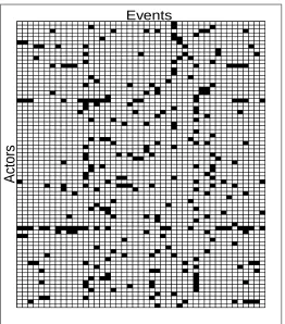
values forms a matrix, called theadjacency matrix, of general dimensionn×r, wherenis the number of actors andrthe number of events. In smaller networks this matrix can be printed and read. For large arrays like the terrorist network it is too large to be readable, and a “map” format is used instead for visualisation. Here the presence of a link (1) in cell (i, j) is shown by a black square, and the absence of a tie (0) by a white square. The map for the terrorist network is shown in Figure 1. The full adjacency matrix is given in the supplementary materials.
Actors
[image:4.595.176.438.121.419.2]Events
Figure 1: Noordin Top network matrix
Husin Top
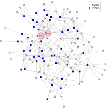
[image:5.595.144.515.145.522.2]Actors Events
Figure 2: Noordin Top network map
3
Data strucures for network analysis
unipar-tite networks, have well-developed methods which however cannot be used for bipartite networks.
A common approach to the analysis of bipartite networks is to convert them to unipartite networks, byprojection of the adjacency matrix Y into its outer productY Y′. For the terrorist network this involves summing over the events
attended, to give a unipartitevalued networkwhose (i, j) entry is the number of eventsjointly attendedby actorsiandj. The “value” would be a count, and not in general a 0 or 1 value. A common further approach is to convert the count to a binary, by dichotomizing the value using some horizon. We discuss in§10 the dangers of this approach, recently pointed out strongly by Neal (2014) and Gerdes (2014).
4
Analyses by Everton
The Noordin Top network is analysed extensively in the chapters of Everton’s book, which is in addition a very detailed manual for network analysis using the major packages (UCINET, Pajek and ORA) developed for this purpose. The bipartite networks considered there are converted to unipartite networks in these analyses. The analyses provide a very detailed examination of the network properties of the standard kinds in social network analysis, and we do not detail them here. (Graphical representations of networks vary among packages.)
We follow a different form of analysis, based on explicit probability models for the bipartite network and its group structure, described in§6. We discuss the conclusions from our analysis, and relate them to those from Everton’s analyses, in§10.
5
The meaning of a group or class
A fundamental question which has to be addressed first is what we mean by a group, in this social context. We should first note than even the word for this subset of actors is not consistent across research fields: it is also called community,cliqueandclass.
We adopt, as in Aitkin, Vu and Francis (2014), the definition of a group or class asan identifiable subset of actors who tend to attend the same events. This definition will be made specific after we consider possible models for the event attendance variables.
6
Statistical models
6.1
Models for a random process
the valueYij = 1 with probability pij, and Yij = 0 with probability 1−pij.
The probability of the pattern of “responses”{yij}given the set of probabilities
{pij} over all actors and all events is
Pr[{yij} | {pij}] =
Y
i
Y
j
pyij
ij (1−pij)1−yij,
assuming (a strong assumption!) the independence of event attendance both within and among actors. We can bring the actor and event structures into the model in several ways. Aitkin, Vu and Francis (2104) gave an extensive list. Here we report on a subset of models used for the terrorist network.
6.2
The Rasch model
The Rasch model is widely used initem response theory (IRT) in psychology. Applied to a network, it is expressed through row and column parameters. Each actori= 1, ..., nhas apropensityθi to attend any event. Each eventj= 1, ..., r
has anattractiveness φj to any actor. Actors attend eventsindependently, and
independently of each other. The Rasch model is a main effect or additive model, in actors and events, on the logit scale:
logitpij = log
pij
1−pij
=θi+φj.1
For the Noordin Top network, the “events” attended by network members include meetings of various kinds (detailed above), and participation in attacks. The actor’s “propensity” to attend events reflects his special or general abilities and level of responsibility.
The Rasch model has no group structurefor actors, and so plays the role of a baseline model for comparison with models with group structure. Other “link” functions could be used instead of the logistic. Caron (2012) considered the complementary log-log link.
6.3
The latent class model
We now switch nomenclature and refer to groups asclasses, as this is the tra-dition in latent class modelling. The use of this model in social networks dates from Holland, Laskey and Leinhardt (1983), though it has been used then and since only for one-mode networks, apart from Aitkin, Vu and Francis (2014). However it is very well-established in sociology for contingency table analysis, from Lazarsfeld and Henry (1968) and Goodman (1974) onwards, and more re-cently for binary incidence matrices at the individual level. The model specifies a K-class latent structurefor actors; the classes are distinguished by different sets of event attractiveness parametersamong classes but identical attractive-ness parameterswithinclasses.
1One of the parameters is unidentifiable in this parametrization: it is usually assumed that
Within each classkthe model fitted is a variation of the Rasch model with class-specific event attractiveness parameters φjk, and class instead of actor
“intercepts”ψk. The model assumes independence between the event attended
within classes; this weakens the assumption of full independence. Marginally (summing over the unobserved classes), the events attended by actors are cor-related, due to the omitted class variable. This unconditional dependence but conditional independence is characteristic of latent variable models, including the classical factor model. Assessing the validity of the conditional indepen-dence assumption is difficult, as for the factor model, since there is in general noexact partition of the actors into the latent classes which would allow this assessment. For sparse data, as in the Noordin Top network, the assessment of conditional independence would have further (lack of data) difficulties.
Replacing pij byqijk to incorporate the latent structure, the formal model
is:
Pr[{Yij} |k, i,{qijk}] = r
Y
j=1
qyij
ijk(1−qijk)
1−yij
Pr[{Yij} |i,{qijk}] = K
X
k=1 πk
r
Y
j=1
qyij
ijk(1−qijk)
1−yij
Pr[{Yij} | {qijk}] = n Y 1=1 K X k=1 πk
r
Y
j=1
qyij
ijk(1−qijk)1−yij
logitqijk = ψk+φjk.
The class intercepts ψk in this model are not identifiable separately from
the event attractiveness parametersφjk without some form of constraints. The
logit model can be represented alternatively asλjk, absorbing the ψk into the
φjk. We make use also of the extended latent class model, retaining individual
actor propensities: logitqijk=θi+φjk.
The probability that actor i is in class k may depend on actor covariates
xi but is independent of the tie variables yij. The model parametersπk, θi or
ψk and φjk do not have to be known or specified; they can be estimated by
now-standard methods, discussed in§§7,8.
An important question is how to determine the number of classesK; this is discussed at length in§8.5.
7
The model likelihood
Statistical models are estimated, assessed and compared through the model likelihood. We have a modelf({yij} | λλλ) for data {yij}, depending on model
parametersλλλ. The likelihood is
For the extended latent group model with K groups, the likelihood follows immediately from the mixture model specification above:
L(λλλ) =
n
Y
1=1
K
X
k=1 πk
r
Y
j=1
qyij
ijk(1−qijk)1−yij
,
logitqijk = θi+φjk,
withλλλ= ({πk},{θi},{φjk}, K).
We present in the remainder of the paper the Bayesian analyis of the model, following Aitkin, Vu and Francis (2014). For reasons discussed in detail there (the greater precision achievable with the Bayesian analysis), we do not present the maximum likelihood analysis.
We examine the following sequence of latent class models of decreasing com-plexity for the logit of the probabilityqijk that actoriattends eventj (itself a
part of scales) in classk.
A: θi+φkj – an extension of the latent class model, with individual actor
propensities and class-specific event attendance parameters;
B:ψk+φkj ≡λkj – the “standard” or “classic” latent class model: the class
intercepts are not separately identifiable from the class-specific event parame-ters;
BS:ψk+φks≡λks – the “scale” version of B;
C:ψk+φj– constrained model B with common event attendance parameters
across classes;
CS:ψk+φs – constrained model BS with common scale parameters across
classes.
8
Bayesian analysis of two-mode networks
8.1
Priors and posteriors
We augment the model likelihood L(λ) by aprior distributionπ(λ|γ) for the model parametersλdepending in general on prior parametersγ, and use Bayes’s theorem to update the prior distribution to theposterior distributionπ(λ|y, γ):
π(λ|y, γ) = R L(λ)·π(λ|γ)
L(λ)·π(λ|γ) dλ.
The denominator is a scaling term, depending on the datayand γbut notλ. If the prior is flat – constant – then the posterior distribution is a simple scaled version of the likelihood. Throughout this paper, following Aitkin (2010) we use flat,referenceor non-informative priors, to allow as far as possible the datato determine the posterior distribution through the likelihood.
way familiar from frequentist inference but without any assumption of normality. The posterior standard deviation is often quoted, though this is useful only for normal posterior distributions.
8.2
Priors for the latent class models
We implemented the Markov chain Monte Carlo (MCMC) procedure in Open-Bugs. We followed the model structures A–CS set out in §7, with minimally informative priors: a Dirichlet (1,1,...,1) prior for the class proportionsπk;
in-dependent normal priors with mean zero and variance 10 for the propensity parametersθi, class interceptsψk and event attendance parametersφj or scale
parametersφs.
After convergence we drew 10,000 random values from their joint posteriors and used every 10th value to reduce serial dependence.
8.3
Posteriors of functions of data and parameters
One of the powerful features of Bayesian analysis is its ability to provide pos-terior inference about complicated functions of the data and parameters. In frequentist theory we have to rely on the delta method – Taylor series expan-sions – to obtain the asymptotic sampling distributions of non-linear functions of the model parameters, especiallyratiosof parameters.
In Bayesian theory this is unnecessary; forposterior samplinginference about a non-linear functiong(λ) of the model parameters, we simply makeM random drawsλ[m] ofλfromπ(λ|y), and substitute them into the functiong, to give
M random drawsg[m]=g(λ[m]) from thefull posterior distribution ofg(λ).
8.4
Posterior distribution of class membership
probabili-ties
A general problem with the use of posterior class membership probabilities from Bayes’s theorem following the EM algorithm is familiar from the frequentist analysis of other complex models. This is the problem of overstated precision resulting from the substitution of ML estimates for true parameter values, with-out any allowance for the imprecision of the ML estimates. In frequentist anal-ysis this is forced on us by the complexity of the exact sampling distributions, especially for non-linear functions of the parameters.
As described above, the posterior distributions of these quantities can be ob-tained in theory from the random draws of the parameters. Recall that the pos-terior probability of membership of caseiin classk, in the generalK-component mixture with componentkdensityfk(y|λk) with component-specfic parameter
λk, is
πki=
πkfk(yi|λk)
PK
ℓ=1πℓfℓ(yi |λℓ)
From the posterior distributions ofλk andπk, we makeM independent draws
λ[km] and π
[m]
k and substitute them intoπkito giveM draws
πki[m]= π [m]
k fk(yi|λ
[m]
k )
PK ℓ=1π
[m]
ℓ fℓ(yi|λ
[m]
ℓ )
.
However, a major issue in computing posterior distributions for any class-specific parameter is label-switching. In the ML estimation of the model pa-rameters, the class labelling of the K class parameter estimates is arbitrary, and causes no confusion. However in the MCMC iterations, the class labelling can vary during iterations and switch the class labels around, leading to class-specific posteriors that are mixtures of the posteriors from each true class. This can lead in the worst case to identical class-specific distributions for all the class parameters, despite convergence.
We follow the approach of Sperrin et al (2010), in which the labels to be attached to the M sets of posterior parameter draws are treated as missing data and analysed with an EM algorithm. For the two-class model, there is almost no uncertainty about the draw labels, but there is considerably more uncertainty with the three- or more class models. We discuss this below.
8.5
Posterior distribution of the model deviance
8.5.1 General models
A particularly useful application of the posterior sampling approach is to the deviance. In Bayesian terms the deviance isD(λ) =−2 logL(λ). Since this is a function of bothλand the datay, it also has a posterior distribution obtainable in this way: givenM random drawsλ[m], we substitute them into the deviance to giveM random drawsD[m] =D(λ[m]).
A full discussion of this approach, and many applications of it, are given in Aitkin (2010). Aitkin, Vu and Francis (2015) carried out a simulation study to evaluate this approach, for both normal mixtures and Bernoulli latent class models. For latent class models, correct identification of many classes required substantial sample sizes of actors, in the simulations based on binary symptoms in psychiatric patients. Our application here is to Bayesian model comparisons of the number of latent classes. A normal mixture example can be found in Chapter 9 of Aitkin (2010).
Within a model type (A, B, BS, C, CS) we haveKpossible models, consist-ing of latent class models withk= 1, ..., K classes, specified byKsets of model parametersλk containing the class proportion parametersπk, the class
propen-sity parametersθk and the class-conditional event attendance parametersφkj,
or scale parametersφks. For eachk we obtain the posterior distribution ofλk,
and the consequent posterior distribution of the devianceDk. The deviance is
unaffected by label-switching, since it is asymmetric functionof the class labels, and invariant under their permutation.
MLEs internal to the parameter space, the second-order Taylor expansion of the deviance D(λ) about the MLE ˆλ gives the posterior distribution of the model deviance, by a Bayesian version of the derivation of the asymptoticχ2
distribution for the likelihood ratio test statistic:
Dk(λk)∼Dk(bλk) +χ2pk,
where pk is the dimension of λk (Aitkin 2010 p. 53). It is notable that the
posterior distributionstarts from the frequentist deviance, since this is minimised over all possible parameter values.
The asymptotic result, if it applies at all, is restricted to the simplest mod-els: null and scale, for which the parameter dimension is small compared to the number of ties. For the mixture models, the actual posterior distributions depart from their asymptotic forms in two respects, as described in Aitkin (2010 pp. 216-220): the distributionsstart from larger values than the frequentist de-viances, because with increasing parameter dimension it is increasingly difficult to sample by chance the MLE; and the distributions aremore diffusethan theχ2
distributions because the parameter posteriors are skewed and/or heavy-tailed. With increasingKthe frequentist deviances for the models (not shown) are increasingly far below the smallest values in the 1,000 draws from the posterior distributions of the model deviances. This phenomenon is discussed in Aitkin, Vu and Francis (2014) – it is the increasing difficulty of randomly sampling parameter values near the MLE asK increases. It shows that the maximized likelihood is not a satisfactory summary of the likelihood evidence for the model, and explains why model comparison procedures based on the maximized log-likelihood – the log-likelihood ratio test, AIC and BIC – are not reliable indicators of model support for heavily parametrized models, especially with sparse data. However, the deviance distributions can in many cases bestochastically or-dered. There are several possibilities, which are illustrated in the next section with the Noordin Top network.
1. Complete stochastic ordering: the deviance cdfs are ordered and do not cross(except merge at 0 and 1); then the leftmost distribution gives the best-preferred model.
2. Partial stochastic ordering: the leftmost distribution does not cross the others, which may cross each other; then the leftmost distribution gives the best-preferred model.
3. No stochastic order: some or all of the distributions cross.
We discuss these further, and give a procedure for discriminating the models, with the analysis of the Noordin Top data.
9
Bayesian analysis of the Noordin Top network
distribution of the class deviances. These are shown for each model in Figures 3–7.
1200 1300 1400 1500 1600 1700 1800 1900
0.0
0.2
0.4
0.6
0.8
1.0
Noordin
Deviance
CDF
[image:13.595.164.441.173.369.2]K=1 K = 2 K = 3 K = 4 K = 5
1650 1700 1750 1800 1850 1900
0.0
0.2
0.4
0.6
0.8
1.0
Noordin
Deviance
CDF
[image:14.595.137.414.135.336.2]K = 1 K = 2 K = 3 K = 4 K = 5
Figure 4: Noordin Top model B deviance distributions
1700 1750 1800 1850 1900
0.0
0.2
0.4
0.6
0.8
1.0
Noordin
Deviance
CDF
K = 1 K = 2 K = 3 K = 4 K = 5
[image:14.595.135.414.397.596.2]1700 1750 1800 1850 1900
0.0
0.2
0.4
0.6
0.8
1.0
Noordin
Deviance
CDF
[image:15.595.137.414.135.336.2]K = 1 K = 2 K = 3 K = 4 K = 5
Figure 6: Noordin Top model C deviance distributions
1750 1800 1850 1900
0.0
0.2
0.4
0.6
0.8
1.0
Noordin
Deviance
CDF
K = 1 K = 2 K = 3 K = 4 K = 5
[image:15.595.136.413.396.594.2]Apart from Figure 3, the deviance graphs show a consistent pattern: the deviance distributions decrease stochastically fromK = 1 toK = 3, and then increase very slowly. These graphs suggest that three classes are established, but not more. Figure 3 shows a different pattern: the deviance distributions decrease stochastically from 1 all the way to 5 classes.
A careful comparison of the deviance scales in the five figures shows that the deviance distributions for 3, 4 and 5 classes with model A are stochastically smaller than the three-class distributions for models B, BS, C and CS (and for any other number of classes).
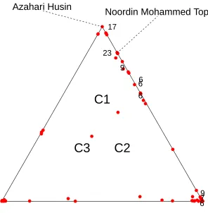
To understand the 3-class and 5-class A models, we compute the membership probabilities for each actor in each class, from the means of the membership indicator variables across the 1,000 random draws. Table 2 in the supplementary materials gives these probabilities for the 3-class model. We give in Figure 8 a ternary plot of these probabilities. The centrepoint of the triangle corresponds to probability 1/3 of membership in each class. Actors at a vertex have probability 1 of belonging to the vertex class. Actors spread along a side of the triangle have non-zero probabilities of belonging to both the vertex classes. Actors in the interior have non-zero probabilities of belonging to all three classes.
The labels (for the number of events attended) are jittered perpendicular to the axes. Labels are placed only for actors for whom the number of events attended is five or more. The membership pattern is unclear. Husin (attending 17 events) defines Class 1, but Top (attending 23 events) is some distance to-wards Class 2. Most of the members attending five or more events are spread out along the Class 1 - Class 2 axis. Class 2 has 22 members attending less than five events, and Class 3 a small group of seven actors clearly identified, with a small number spread along the Class 2 - Class 3 axis, and two members on the Class 3 - Class 1 axis. Several actors are in the interior of the triangle, with very diffuse membership probabilities. So the nature of the three classes (in terms of membership) is unclear.
The five-class model is even more unclear. Table 3 in the supplementary materials shows that the small Class 5 has only four clearly identified (proba-bility 1.00) members (i = 7, 9, 63 and 73), all with degree (number of events attended) 5 or 6. Class 1 is also sparse, with nine clearly identified members (i
C1
C2
C3
Azahari Husin
17
Noordin Mohammed Top
23
7
6
9
9
6
6
6
P
S
fr
a
[image:17.595.153.449.132.434.2]g
Figure 8: Three-class membership probabilities, Model A
9.1
Modelling the prior
Most of the latent class models considered here are heavily parametrised, and the flat priors on the parameters do not change this. The sparse data from the adjacency matrix provide little information about these unrelated parameters. A general Bayesian approach to heavily parametrised models is to use priors which replace the unrelated parameters by adistributional model with a small number of parameters. This approach is widely used in all fields of random effect modelling, including Rasch modelling (de Boeck 2008), though it is not so widely used in latent class analysis.
We evaluate this approach, and its effect on the interpretation of the latent classes, bymodelling the class and event parameters. We write sas before for scale, and change slightly the model notation from§7 to: yijsk = 1 if actoriin
classes andφsj for events within scales, and use the model
logitqijsk =ψk+φsj
ψk ∼N(µψ, σψ2)
φsj∼N(µφ, σ2φ)
and priors
µψ ∼N(0,4)
σψ2 ∼U(0,2)
µφ∼N(0,100)
σ2φ∼U(0,10).
For the membership indicator variables we use the same diffuse multinomial/Dirichlet model and prior as in the previous analysis:
Zik ∼M(1, π)
π∼D(1,1, ...,1).
We call this model therandom Rasch latent class model.
The likelihood now contains the additional unobserved “random effect” terms
ψk andφsj, which have to be integrated out of the likelihood with respect to
their model distributions, leaving the likelihood as a function of the prior param-etersµψ, σ2ψ, µφ, σφ2. As with the frequentist “fixed effect” and “random effect”
models, this likelihood is not comparable with the “fixed effect” likelihood with flat priors on all the parameters, so the deviance scales for these two different models will not be comparable.
1680 1700 1720 1740 1760 1780 1800
0.0
0.2
0.4
0.6
0.8
1.0
Deviance
CDF
Rasch Rasch K = 2 Rasch K = 3 Rasch K = 4 Rasch K = 5
P
S
fr
a
[image:19.595.138.448.149.407.2]g
Figure 9: Noordin Top network deviance distributions, random Rasch latent class model
The deviance distributions improve (move left) substantially from the Rasch through the 2-class to the 3-class model. The distributions for 3, 4 and 5 classes overlap almost completely. Three classes are clearly established, while the fourth and fifth give unnecessary complexity.
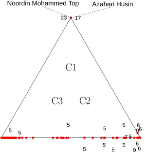
Figure 10 shows a ternary plot of membership probabilities in the 3-class model, with labels (for the number of events attended) jittered perpendicular to the axes. Labels are placed only for actors for whom the number of events attended is five or more.
●
●●● ● ● ● ● ● ●
●
● ●●
● ● ●● ●
●
●
●
●●●●● ●● ●
●●●●● ●●●●●● ● ●● ●● ● ● ● ●● ● ●
●
● ●
● ●
● ● ●
●● ● ● ●
● ● ●●● ● ● ●
Azahari Husin
17
Noordin Mohammed Top
23
7
6
5
9
5
5
5
5
5
5
9
5
6
6
5
5
6
C1
[image:20.595.153.451.134.447.2]C2
C3
Figure 10: Three-class membership probabilities, random Rasch model
A natural question, given the infrequency of appearance of most actors at any event, is whether there is a real difference between classes 2 and 3 in the frequency profiles of their event participation. To address this this we give in the supplementary materials graphs of the posterior distributions of the event attendance probabilities for all three classes, broken down by the event scales.
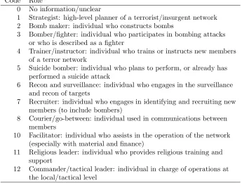
Code Role
0 No information/unclear
1 Strategist: high-level planner of a terrorist/insurgent network 2 Bomb maker: individual who constructs bombs
3 Bomber/fighter: individual who participates in bombing attacks or who is described as a fighter
4 Trainer/instructor: individual who trains or instructs new members of a terror network
5 Suicide bomber: individual who plans to perform, or already has performed a suicide attack
6 Recon and surveillance: individual who engages in the surveillance and recon of targets
7 Recruiter: individual who engages in identifying and recruiting new members (to include bombers)
8 Courier/go-between: individual used in communications between members
10 Facilitator: individual who assists in the operation of the network (especially with material and finance)
11 Religious leader: individual who provides religious training and support
[image:21.595.134.479.130.390.2]12 Commander/tactical leader: individual in charge of operations at the local/tactical level
Table 1: Actor roles from Everton
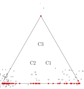
Figure 11 shows the 74 actors identified by the 13 role labels given by Everton (2012 p. 396) in Table 1. The labels are jittered away from the axes.
Notable differences between the 21 members of Class 2 and the 51 members of Class 3 (as assessed by the largest posterior probability) are that all seven suicide bombers, and 11 of the 14 bomber/fighters, are in Class 3, while 5 of the 7 couriers are in Class 2. The other role categories do not differ substan-tially between classes. Our interpretation of this analysis is that, allowing for possible progression in actor roles following actions, Class 2 are the “Trainers”, intermediaries between the planners and operations directors in Class 1, and the “footsoldiers” in Class 3 carrying out the operations.
10
Comparisons with Everton’s analyses
7 10 1 1 11 1 4 12 11 1 11 8 1 12 4 5 5 12 11 5 2 11 3 8 3 3 12 8 3 10 12 3 4 3 5 2 3 3 5 10 4 3 12 7 10 6 11 5 3 4 10 12 10 1 8 4 4 10 5 3 4 10 3 8 8 3 10 8 4 3 4 7 10 1
C1
C2
C3
Figure 11: Three-class membership probabilities by roles, random Rasch model
models is not implemented in the packages used for his analyses.
The closest comparison is in Chapter 6 “Cohesion and Clustering” which considers the identification of cohesive subgroups. Everton evaluates four sets of algorithms for detecting subgroups: components, cores, factions, and Newman groups. An immediate difficulty with these comparisons is that some of the analyses are applied to different sub-networks of actors: the “alive” network has 69 actors, but the “alive and free” network has only 24: 45 actors are imprisoned.
A further difficulty is that the ties themselves are of several kinds, and all the analyses are of one-mode networks, by collapsing the adjacency matrix across events (formally, by transforming the n×p adjacency matrixY to the n×n
in common by pairs of actors were further dichotomized for procedures which required binary data. This differs fundamentally from the latent class analysis, which requires the full information in the adjacency matrix.
The difficulty with this approach is clear. Summing over the event classi-fication gives an entryni,i′ in cell (i, i′) of the resulting projected table, given byni,i′ =P
r
j=1yijyi′j, a sum of products of Bernoulli variables which has no
simple form. Dichotomising this sum will make the distribution even more com-plex. Gerdes (2014) and Neal (2014) discuss this problem at length and suggest some alternatives, though the direct modelling of the bipartite table is not one of them.
A summary of the results reported by Everton follows; we do not give details of the algorithms used.
The components analysis of the “aggregated trust network” in Pajek placed all actors in the one component.
The “alive” network gave the same single component.
Thek-core analysis of the “alive trust” network in UCINET showed a well-connected central subgroup surrounded by four slightly less well-connected sub-groups.
Thek-core analysis of the “alive operational” network found a set of clusters centering on Noordin Top.
The faction analysis in UCINET of the “alive and free” combined network gave 8, 9 or 3 factions depending on the “measure-of-fit” option chosen; other considerations suggested 3 or 4 factions.
The Newman group analysis gave similar results to the faction analysis for the “alive and free” combined network.
This does not exhaust the list of possible algorithms for subgroup structure; as Everton wrote (p. 204),
There are several more we have not considered. What should be clear by now is that we may have to use multiple algorithms before we succeed in detecting cohesive subgroups. ..
11
Conclusions
It may be frustrating to readers that there is little connection between our analyses and those of Everton. This lack of connection follows from the different latent-class model-based approach we are following. The multiple algorithms for subgroup structure examined by Everton do not lead to any clear subgroup structure. In our view this is a consequence of analysing the one-mode data structure, with its loss of information.
obscure the connections among them, the identification of the leaders is clear, and we can give a plausible interpretation of the “command structure” of the network from the three-class model.
A possibility not considered in our paper is the modelling of change over time in the terrorist network structure. This comes about through the time-stamping of membership of the actors: over the period 2000-2010 we know the first time at which an actor is mentioned, and so is known to have entered the network. We know also when actors die or are arrested and therefore are withdrawn from the network. However the events at which attendance is recorded are not time-stamped, so we cannot model the successive structures of the network, and changes to it, as each new event occurs. If the events were also time-stamped, much richer modelling would be possible.
An extension not considered in this paper is biclustering, or double latent-class modelling of both actors and events. In the Noordin Top network, the reason is clear: we have Everton’s manifest categorization of events by scales. In other bipartite networks, biclustering may be of interest. The observed data likelihood in this model is particularly complex, though MCMC analysis is fairly straightforward. Large networks will require very long computation times for large models with many latent classes; variational methods are increasingly used for such networks. Most variational methods are developed for the symmetric unipartite network model (for example Bickel et al 2013). Vu, Hunter and Schweinberger (2013) and Vu and Aitkin (2015) give examples for bipartite networks.
12
Acknowledgements
In preparing this paper we have benefitted greatly from interactions with the Social Network group in the Department of Psychology, School of Psychologi-cal Sciences at the University of Melbourne. Professors Pip Pattison (a former Deputy Vice-Chancellor of the University) and Garry Robins have been particu-larly helpful in comparing and interpreting the differences between this approach and others used in social network modelling, especially the exponential random graph model approach.
We are also grateful for assistance from Sean Everton, and research support from the Australian Research Council under Grant DP120102902 for Pip Patti-son’s participation in the project, the support of Duy Vu for the period of this research (2012-15), and visits to Melbourne from the University of Lancaster by Brian Francis.
13
References
Aitkin, M. (2010). Statistical Inference: an Integrated Bayesian/Likelihood Approach. Boca Raton FL: Chapman and Hall/CRC Press.
Aitkin, M., Vu, D. and Francis, B.J. (2014). Statistical modelling of the group structure of social networks. Social Networks 38, 74–87.
Aitkin, M., Vu, D. and Francis, B.J. (2015). A new Bayesian approach for determining the number of components in a finite mixture. Metron 73, 155–176.
Bickel, P., Choi, D., Chang, X. and Zhang, H. (2013). Asymptotic normality of maximum likelihood and its variational approximation for stochastic blockmodels. Annals of Statistics 41, 1922-1943.
Davis, A., Gardner, B.B. and Gardner, M.R. (1941). Deep South: A Social Anthropological Study of Caste and Class. Chicago: University Press.
De Boeck, P. (2008). Random item IRT models. Psychometrika 73, 533-559.
Everton, S.F. (2012). Disrupting Dark Networks. Cambridge: University Press.
Gerdes, L.M. (2014) MAPPing dark networks: a data transformation method to study clandestine organizations. in Network Science, Cambridge Uni-vesity Press, pp. 1–41.
Goodman, L.A. (1974). Exploratory latent structure analysis using both iden-tifiable and unideniden-tifiable models. Biometrika 61, 215–231.
International Crisis Group (2009). Indonesia: Noordin Top’s Support Base. Asia briefing 95. Online at
http://www.crisisgroup.org/~/media/Files/asia/south-east-asia /b95_indonesia_noordin_tops_support_base.pdf
Lazarsfeld, P.F. and Henry, N.W. (1968). Latent Structure Analysis. Boston: Houghton Mifflin.
Neal, Z. (2014) The backbone of bipartite projections: inferring relationships from co-authorship, co-sponsorship, co-attendance and other co-behaviors. Social Networks 39, 84–97.
Sperrin, M., Jaki, T. and Wit, E. (2010). Probabilistic relabelling strategies for the label switching problem in Bayesian mixture models. Statistics and Computing 20, 357–366.
Vu, D. and Aitkin, M. (2015). Variational algorithms for biclustering models. Computational Statistics and Data Analysis 89, 12–24.
Statistical modelling of a terrorist network –
supplementary materials
June 12, 2016
Murray Aitkin and Duy Vu School of Mathematics and Statistics University of Melbourne, Victoria Australia
and Brian Francis
Department of Mathematics and Statistics
Lancaster University, Lancaster LA14YF United Kingdom %sectionAppendix
2
3-class posterior membership probabilities
i\C 3 2 1 d i\C 3 2 1 d
1 0.05 0.95 0.00 1 41 0 1 0 5
2 0.63 0.37 0 3 42 0.04 0 0.96 5
3 0 1 0 7 43 0 1 0 9
4 0.19 0.80 0.01 2 44 0 0.05 0.95 4
5 0.30 0.67 0.03 3 45 0 0.99 0.01 3
6 0.02 0.16 0.82 3 46 0.02 0.23 0.75 1
7 0 0.38 0.62 6 47 0.66 0.32 0.02 2
8 0.01 0.32 0.67 1 48 0 0.15 0.85 2
9 0 0.38 0.62 5 49 1.00 0 0.00 4
10 0.17 0.32 0.51 3 50 0.04 0 0.96 3
11 0.00 1.00 0 3 51 0 1 0 5
12 0 0.20 0.80 9 52 0.02 0.97 0.01 2
13 0.04 0.96 0.00 1 53 0.01 0.41 0.58 1
14 0.04 0.96 0.00 1 54 0 0.15 0.85 23
15 0.98 0.01 0.01 2 55 0 0.99 0.01 6
16 0 0.15 0.85 2 56 0 0.15 0.85 3
17 0 1 0 4 57 0.02 0.98 0 2
18 0 1 0 3 58 0.01 0.43 0.56 1
19 0 1 0 5 59 0 0.15 0.85 2
20 0.60 0 0.40 2 60 0 1 0 3
21 0 0 1 17 61 0 1 0 4
22 0 0.70 0.30 3 62 0.61 0.00 0.39 2
23 0.01 0.99 0 3 63 0 0.38 0.62 6
24 0 0.04 0.96 5 64 0 0.04 0.96 3
25 0 1 0 2 65 0 0.94 0.06 5
26 0.98 0.02 0.00 3 66 0.59 0.00 0.41 2
27 0 1 0 3 67 0.99 0 0.01 4
28 0.05 0.95 0.00 1 68 0 0.98 0.02 5
29 0.37 0.26 0.37 1 69 0 0.99 0.01 4
30 0.15 0.85 0.00 1 70 0.99 0.01 0.00 3
31 1 0 0 4 71 0.00 1.00 0 2
32 0 1 0 5 72 0 0.98 0.02 4
33 0 1 0 3 73 0 0.38 0.62 6
34 0.00 0.99 0.01 1 74 0.04 0.94 0.02 2
35 0 1 0 5
36 0 0.26 0.74 4
37 0 0.27 0.73 2 38 0.99 0.01 0 4 39 0.86 0.14 0.00 2
40 0 1 0 2
[image:29.595.135.419.160.624.2]T 12.84 38.90 22.26
3
5-class posterior membership probabilities
i\C 1 2 3 4 5 d i\C 1 2 3 4 5 d
1 0.00 0.32 0.00 0.68 0.00 1 41 0.00 0.00 0.00 1.00 0.00 5 2 0.00 0.93 0.00 0.07 0.00 3 42 0.00 0.04 0.96 0.00 0.00 5
3 1.00 0.00 0.00 0.00 0.00 7 43 0.00 0.00 0.00 1.00 0.00 9 4 0.00 0.69 0.00 0.31 0.00 2 44 0.00 0.00 1.00 0.00 0.00 4
5 0.00 0.98 0.00 0.02 0.00 3 45 1.00 0.00 0.00 0.00 0.00 3 6 0.00 0.10 0.90 0.00 0.00 3 46 0.00 0.04 0.92 0.03 0.01 1
7 0.00 0.00 0.00 0.00 1.00 6 47 0.00 1.00 0.00 0.00 0.00 2 8 0.00 0.04 0.74 0.03 0.19 1 48 0.00 0.00 1.00 0.00 0.00 2 9 0.00 0.00 0.00 0.00 1.00 5 49 0.00 1.00 0.00 0.00 0.00 4
10 0.00 0.98 0.01 0.00 0.00 3 50 0.00 0.04 0.96 0.00 0.00 3 11 0.00 0.00 0.00 1.00 0.00 3 51 1.00 0.00 0.00 0.00 0.00 5
12 0.00 0.00 1.00 0.00 0.00 9 52 0.06 0.90 0.01 0.03 0.00 2 13 0.00 0.32 0.00 0.68 0.00 1 53 0.00 0.02 0.73 0.20 0.05 1
14 0.00 0.33 0.00 0.67 0.00 1 54 0.00 0.00 1.00 0.00 0.00 23 15 0.00 1.00 0.00 0.00 0.00 2 55 1.00 0.00 0.00 0.00 0.00 6 16 0.00 0.00 1.00 0.00 0.00 2 56 0.00 0.00 1.00 0.00 0.00 3
17 0.00 0.00 0.00 1.00 0.00 4 57 0.00 0.01 0.00 0.99 0.00 2 18 1.00 0.00 0.00 0.00 0.00 3 58 0.00 0.02 0.75 0.18 0.05 1
19 1.00 0.00 0.00 0.00 0.00 5 59 0.00 0.00 1.00 0.00 0.00 2 20 0.00 0.70 0.30 0.00 0.00 2 60 1.00 0.00 0.00 0.00 0.00 3
21 0.00 0.00 1.00 0.00 0.00 17 61 0.00 0.00 0.00 1.00 0.00 4 22 0.00 0.00 0.12 0.88 0.00 3 62 0.00 0.67 0.33 0.00 0.00 2 23 0.00 0.02 0.00 0.98 0.00 3 63 0.00 0.00 0.00 0.00 1.00 6
24 0.00 0.00 1.00 0.00 0.00 5 64 0.00 0.00 1.00 0.00 0.00 3 25 1.00 0.00 0.00 0.00 0.00 2 65 0.00 0.00 0.00 0.01 0.99 5
26 0.00 1.00 0.00 0.00 0.00 3 66 0.00 0.68 0.32 0.00 0.00 2 27 0.00 0.00 0.00 1.00 0.00 3 67 0.00 1.00 0.00 0.00 0.00 4
28 0.00 0.33 0.00 0.67 0.00 1 68 0.00 0.00 0.04 0.91 0.05 5 29 0.00 0.56 0.35 0.09 0.00 1 69 0.00 0.00 0.01 0.99 0.00 4
30 0.00 0.34 0.00 0.66 0.00 1 70 0.00 1.00 0.00 0.00 0.00 3 31 0.00 1.00 0.00 0.00 0.00 4 71 0.02 0.85 0.00 0.13 0.00 2 32 1.00 0.00 0.00 0.00 0.00 5 72 0.00 0.00 0.00 0.98 0.02 4
33 0.00 0.00 0.00 1.00 0.00 3 73 0.00 0.00 0.00 0.00 1.00 6 34 0.20 0.04 0.02 0.73 0.00 1 74 0.06 0.92 0.00 0.02 0.00 2
35 0.00 0.00 0.00 1.00 0.00 5 36 0.00 0.00 0.77 0.01 0.22 4
37 0.00 0.00 0.93 0.07 0.00 2 38 0.00 1.00 0.00 0.00 0.00 4 39 0.00 0.97 0.00 0.03 0.00 2
40 0.44 0.00 0.02 0.49 0.05 2
[image:30.595.135.544.159.631.2]T 9.78 19.84 19.19 19.54 5.63 73.98
4
Event-and class-specific posterior distributions
of probabilities of event attendance
0
0 0.5 1
C 1 − Event 1
0
0 0.5 1
C 1 − Event 2
0
10
0 0.5 1
C 2 − Event 1
0
0 0.5 1
C 2 − Event 2
0
10
20
0 0.5 1
C 3 − Event 1
0
10
20
0 0.5 1
[image:31.595.138.486.179.467.2]C 3 − Event 2
0
0 0.5 1
C 1 − Event 1
0
0 0.5 1
C 1 − Event 2
0
0 0.5 1
C 1 − Event 3
0
10
0 0.5 1
C 2 − Event 1
0
10
0 0.5 1
C 2 − Event 2
0
10
0 0.5 1
C 2 − Event 3
0
0 0.5 1
C 3 − Event 1
0
10
0 0.5 1
C 3 − Event 2
0
10
0 0.5 1
[image:32.595.136.490.126.416.2]C 3 − Event 3
0
0 0.5 1
C 1 − Event 4
0
0 0.5 1
C 1 − Event 5
0
10
0 0.5 1
C 2 − Event 4
0
10
0 0.5 1
C 2 − Event 5
0
10
0 0.5 1
C 3 − Event 4
0
10
0 0.5 1
[image:33.595.133.489.122.418.2]C 3 − Event 5
0
0 0.5 1
C 1 − Event 1
0
0 0.5 1
C 1 − Event 2
0
0 0.5 1
C 1 − Event 3
0
0 0.5 1
C 1 − Event 4
0
10
0 0.5 1
C 2 − Event 1
0
0 0.5 1
C 2 − Event 2
0
0 0.5 1
C 2 − Event 3
0
0 0.5 1
C 2 − Event 4
0
10
20
0 0.5 1
C 3 − Event 1
0
10
20
0 0.5 1
C 3 − Event 2
0
10
20
0 0.5 1
C 3 − Event 3
0
10
20
0 0.5 1
[image:34.595.132.491.122.418.2]C 3 − Event 4
0
0 0.5 1
C 1 − Event 5
0
0 0.5 1
C 1 − Event 6
0
0 0.5 1
C 1 − Event 7
0
0 0.5 1
C 2 − Event 5
0
0 0.5 1
C 2 − Event 6
0
10
0 0.5 1
C 2 − Event 7
0
10
20
0 0.5 1
C 3 − Event 5
0
10
20
0 0.5 1
C 3 − Event 6
0
10
20
0 0.5 1
[image:35.595.136.491.126.417.2]C 3 − Event 7
0
0 0.5 1
C 1 − Event 1
0
0 0.5 1
C 1 − Event 2
0
0 0.5 1
C 1 − Event 3
0
0 0.5 1
C 1 − Event 4
0
10
0 0.5 1
C 2 − Event 1
0
10
0 0.5 1
C 2 − Event 2
0
10
0 0.5 1
C 2 − Event 3
0
10
0 0.5 1
C 2 − Event 4
0
0 0.5 1
C 3 − Event 1
0
10
0 0.5 1
C 3 − Event 2
0
10
0 0.5 1
C 3 − Event 3
0
10
0 0.5 1
[image:36.595.133.491.121.417.2]C 3 − Event 4
0
0 0.5 1
C 1 − Event 5
0
0 0.5 1
C 1 − Event 6
0
0 0.5 1
C 1 − Event 7
0
0 0.5 1
C 1 − Event 8
0
0 0.5 1
C 2 − Event 5
0
10
0 0.5 1
C 2 − Event 6
0
10
0 0.5 1
C 2 − Event 7
0
10
0 0.5 1
C 2 − Event 8
0
0 0.5 1
C 3 − Event 5
0
10
0 0.5 1
C 3 − Event 6
0
10
0 0.5 1
C 3 − Event 7
0
10
0 0.5 1
[image:37.595.133.492.122.417.2]C 3 − Event 8
0
0 0.5 1
C 1 − Event 1
0
0 0.5 1
C 1 − Event 2
0
0 0.5 1
C 1 − Event 3
0
0 0.5 1
C 1 − Event 4
0
10
0 0.5 1
C 2 − Event 1
0
10
0 0.5 1
C 2 − Event 2
0
10
0 0.5 1
C 2 − Event 3
0
10
0 0.5 1
C 2 − Event 4
0
10
0 0.5 1
C 3 − Event 1
0
10
20
0 0.5 1
C 3 − Event 2
0
10
20
0 0.5 1
C 3 − Event 3
0
10
20
0 0.5 1
[image:38.595.133.492.123.418.2]C 3 − Event 4
0
0 0.5 1
C 1 − Event 5
0
0 0.5 1
C 1 − Event 6
0
0 0.5 1
C 1 − Event 7
0
0 0.5 1
C 1 − Event 8
0
10
0 0.5 1
C 2 − Event 5
0
10
0 0.5 1
C 2 − Event 6
0
10
0 0.5 1
C 2 − Event 7
0
10
0 0.5 1
C 2 − Event 8
0
10
20
0 0.5 1
C 3 − Event 5
0
10
20
0 0.5 1
C 3 − Event 6
0
10
20
0 0.5 1
C 3 − Event 7
0
10
20
0 0.5 1
[image:39.595.133.492.124.418.2]C 3 − Event 8
0
0 0.5 1
C 1 − Event 9
0
0 0.5 1
C 1 − Event 10
0
0 0.5 1
C 1 − Event 11
0
10
0 0.5 1
C 2 − Event 9
0
10
0 0.5 1
C 2 − Event 10
0
10
0 0.5 1
C 2 − Event 11
0
10
0 0.5 1
C 3 − Event 9
0
10
20
0 0.5 1
C 3 − Event 10
0
10
20
0 0.5 1
[image:40.595.133.494.122.419.2]C 3 − Event 11
0
0 0.5 1
C 1 − Event 1
0
0 0.5 1
C 1 − Event 2
0
0 0.5 1
C 1 − Event 3
0
0 0.5 1
C 1 − Event 4
0
10
0 0.5 1
C 2 − Event 1
0
10
0 0.5 1
C 2 − Event 2
0
10
0 0.5 1
C 2 − Event 3
0
10
0 0.5 1
C 2 − Event 4
0
10
20
0 0.5 1
C 3 − Event 1
0
20
0 0.5 1
C 3 − Event 2
0
20
0 0.5 1
C 3 − Event 3
0
20
0 0.5 1
[image:41.595.135.493.126.416.2]C 3 − Event 4
0
0 0.5 1
C 1 − Event 5
0
0 0.5 1
C 1 − Event 6
0
0 0.5 1
C 1 − Event 7
0
0 0.5 1
C 1 − Event 8
0
10
0 0.5 1
C 2 − Event 5
0
10
0 0.5 1
C 2 − Event 6
0
10
0 0.5 1
C 2 − Event 7
0
10
0 0.5 1
C 2 − Event 8
0
20
0 0.5 1
C 3 − Event 5
0
20
0 0.5 1
C 3 − Event 6
0
20
0 0.5 1
C 3 − Event 7
0
20
0 0.5 1
[image:42.595.133.492.122.418.2]C 3 − Event 8
0
0 0.5 1
C 1 − Event 9
0
0 0.5 1
C 1 − Event 10
0
0 0.5 1
C 1 − Event 11
0
0 0.5 1
C 1 − Event 12
0
10
0 0.5 1
C 2 − Event 9
0
10
0 0.5 1
C 2 − Event 10
0
10
0 0.5 1
C 2 − Event 11
0
10
0 0.5 1
C 2 − Event 12
0
20
0 0.5 1
C 3 − Event 9
0
20
0 0.5 1
C 3 − Event 10
0
20
0 0.5 1
C 3 − Event 11
0
20
0 0.5 1
[image:43.595.133.492.122.418.2]C 3 − Event 12