A tuning method of active disturbance rejection control for a class of high order processes

warwick.ac.uk/lib-publications

Manuscript version: Author’s Accepted Manuscript

The version presented in WRAP is the author’s accepted manuscript and may differ from the

published version or Version of Record.

Persistent WRAP URL:

http://wrap.warwick.ac.uk/117270

How to cite:

Please refer to published version for the most recent bibliographic citation information.

If a published version is known of, the repository item page linked to above, will contain

details on accessing it.

Copyright and reuse:

The Warwick Research Archive Portal (WRAP) makes this work by researchers of the

University of Warwick available open access under the following conditions.

Copyright © and all moral rights to the version of the paper presented here belong to the

individual author(s) and/or other copyright owners. To the extent reasonable and

practicable the material made available in WRAP has been checked for eligibility before

being made available.

Copies of full items can be used for personal research or study, educational, or not-for-profit

purposes without prior permission or charge. Provided that the authors, title and full

bibliographic details are credited, a hyperlink and/or URL is given for the original metadata

page and the content is not changed in any way.

Publisher’s statement:

Please refer to the repository item page, publisher’s statement section, for further

information.

Abstract—_{This paper aims to propose a quantitative} tuning method for active disturbance rejection control (ADRC) that controls the K/(Ts+1)n_{-type high-order}

processes. An asymptote in the Nyquist curve has been observed for the first time and its mathematical expression has been deduced. An asymptote condtion is provided in order to derive a parameter tuning rule under the sensitivity constraint. Although this proposed tuning rule is originally designed for a certain type of high-order processes, it can be extended to other types processes that can be approximated into the form of K/(Ts+1)n_.

Comparisons with different PID control strategies have been conducted for a range of cases to demonstrate the efficiency of the proposed tuning method. Finally, the effectiveness of the proposed tuning rule is experimentally verified on water tank system that exhibits high-order dynamics. Field tests on the superheater steam temperature control of a circulating fluidized bed (CFB) power plant further demonstrate its potential for applications in complex industrial processes.

Index Terms—Active Disturbance Rejection Control, high-order processes, parameter tuning, steam temperature control, maximum sensitivity.

I. INTRODUCTION

igh-order systems represent a common feature existing in many industrial processes, such as the superheater steam temperature and main steam pressure control in power plants[1][2][3]. In fact, many complex industrial processes with nonlinear dynamics are inherently of high-order [4]. Transfer function approximation for a distributed parameter system often results in a high-order model representation [5]. However, designing high-order controllers for high-order processes brings complexities in control analysis, control algorithm implementation and parameter tuning. Therefore, in industrial practice, lower order controllers are usually preferred. For instance, it is reported that more than 94% of the controllers configured in power plant in Guangdong province, China, are lower order PI controllers [6]. When the low order controller is

_{Manuscript received June 03, 2018; revised October 07, 2018 and}

January 30, 2019; accepted March 08, 2019. This work was supported by the National Key Research and Development Program of China, 2016YFB0901405 and the National Natural Science Foundation of China, 51876096. (Corresponding author: Donghai Li.)

T. He, Z. Wu and D. Li are with the State Key Lab of Power Systems, Department of Energy and Power Engineering, University of Tsinghua, Beijing 100084, China (e-mail: he-t14@mails.tsinghua.edu.cn; wu-zl15@mails.tsinghu.edu.cn; lidongh@mail. tsinghua.edu.cn).

J. Wang is with the School of Engineering, University of Warwick, Coventry CV4 7AL, U.K. (e-mail: jihong.wang@warwick.ac.uk).

used, higher-order dynamics are often considered as a part of the internal disturbances. Besides, various external disturbances and uncertainties are inevitable in industrial processes, such as variation in fuel quality, load change, environmental temperature and pressure changes. Conventional PI/PID controllers are found inadequate in dealing with all kind of disturbances in many cases, thus efficient anti-disturbance techniques need to be applied in industrial control [7].

Active disturbance rejection control (ADRC) is one of the notable disturbance/uncertainty estimation and attenuation techniques [8]. ADRC is firstly proposed by Han [9] to serve as an alternative control to the classical PID [10]. The extended state observer (ESO), the core part of ADRC, estimates the internal uncertainties (the un-modeled dynamics, the higher-order dynamics, and parameter errors) and the external disturbances as a lumped term called the total disturbance, which is then compensated via control actions in real time. During the last two decades, ADRC has been extensively investigated and applied by many researchers in different countries and in different industrial sectors [11]. The theoretical analysis of ADRC with regard to convergence and stability proof have been studied in [12][13]. Performance and properties of ADRC have been analyzed in frequency domain [14]. Improved ADRC have been proposed to address the challenges caused by large time-delays [15], non-minimum phase [16], and multi-variable coupling [17][18]. ADRC were initially studied via simulations and experiments and then extended to industrial applications with the range from motion control [19], electronic and mechanical systems [20] to process control [21].

Control parameter tuning is a key factor for ADRC’s successful implementation in real industrial processes. However, there are no well-established quantitative tuning rules for ADRC parameters, especially for high-order processes. Most of the tuning work is performed manually, although the process of trial and error is tedious, and in some cases, frustrating. There are successful attempts using heuristic algorithms to optimize parameters [2][22], but the tuning process is time-consuming and not convenient enough for industrial sectors to adopt. An important progress was made by Gao [23] in 2006. The bandwidth-parameterization in [23] had greatly simplified the tuning process by reducing six tuning parameters to three. Chen [24] graphically presented the stable region of second-order ADRC parameters and refined the tuning process in the sight of closed loop desired dynamics. Wang [25] proposed a particular ADRC tuning method for time-delay systems. However, those studies on parameter

Ting He, Zhenlong Wu, Donghai Li and

Jihong Wang,

Senior Member IEEE

A Tuning Method of Active Disturbance

Rejection Control for a Class of High-order

Processes

tuning gave little attention to high-order processes with no consideration to the sensitivity constraint, such as the maximum sensitivity Ms, which is a dominant robustness index

in control design.

To address the challenges in ADRC parameter tuning, in this work, an asymptote condition is used to constrain the maximum sensitivity of the control system. Based on the asymptote condition, a new quantitative one-parameter-tuning rule is proposed for ADRC used in high-order processes. The proposed tuning method has demonstrated the following advantages: 1) the explicit tuning formulas are simple and easy to use; 2) there is a tuning parameter to trade-off between performance and robustness; 3) the proposed method can be easily extended to other types of processes.

The rest of this paper is organized as follows. The problem is formulated in Section II. Section III describes the derivation of the tuning rule. In Section IV, comparative simulations are performed on various types of processes. Laboratory experiments of a water tank system and field tests in a circulating fluidized bed (CFB) power plant are carried out to verify the effectiveness of this tuning methods in section V. Conclusions are given in Section VI.

II. PROBLEM FORMULATION

For derivation of tuning rules, the process is assumed to be in the form of high-order, K



Ts1



n. Model parameterK T, , andnwill be incorporated in the derivation of the tuning rule. The second-order ADRC is used as an example to show how the low-order ADRC controls high-order process. The tuning rules of first-order ADRC can be easily derived based the method introduced. Due to page limit, the stability analysis of the second-order ADRC controlling high-order process is presented in Supplementary materials. The schematic diagram is shown in Fig. 1, from which the second-order ADRC is formulated by the state feedback control, the extended state observer (ESO), and the real time disturbance compensation.

Gp

ESO +

d

-r u y

kp _-

-z1

z2

z3

kd

1/b0

[image:3.612.76.272.474.544.2]

u0

Fig. 1. The schematic diagram of second-order linear ADRC For the second-order ADRC, the process can be formulated into the canonical form of two cascaded integrators, with the external disturbanced , noise w , nonlinear and high-order dynamics lumped in the total disturbance f .

 





1 2

2 1 2 1 0

3

1 2 3

, , , , ,

, ,

n

x x

x f x x x d w b u x f

y x y x f x

 

 _{ }

 

 

  

(1)

The ESO is designed based on the above canonical form, so the mathematical expression of the ESO is presented in (2), where ₁, ₂ and ₃ are the observer gains andb₀is the input gain.













1 2 1 1

2 3 2 1 0

3 3 1

z z y z z z y z b u z y z

  

  

 

   



  



(2)

The ESO statesz₁andz₂are used for feedback control. k_p

andk_dare the feedback control parameters.





0 p 1 d 2

u k rz k z (3) State z₃ is the estimated total disturbance, and it is compensated in real time by



0 3



0.

u u z b (4) The second-order ADRC has six parametersk k b_p, _d, ₀, ₁, ₂ and ₃ . The bandwidth-parameterization [23] has greatly simplified the tuning process. It makesk_p,k_das a function of the desired closed-loop bandwidth _c and   ₁, ₂, ₃ as a function of ESO bandwidth_o.

2 2 3

1 2 3

, 2 , 3 , 3 ,

p c d c o o o

k 



k 

 



 



 





(5) It leaves three parameters c, oandb0to tune. However, it is still not easy to find three proper values for c, oandb0. Therefore, there is a demand for developing an efficient ADRC tuning rule that can reduce the workload of manual tuning.

III. DESIGN PROCEDURE

A. The sensitivity constraint

In process control design, the models used for controller design are often imprecise, and the process parameters and dynamics change with time and also operating conditions. Therefore, it is desired that the control system should be insensitive to the process variations and disturbances. The maximum sensitivity M_s and Maximum complementary sensitivityM_tare typical measures of sensitivity to process variation [26]. This paper uses maximum sensitivity M_s constraint to develop a parameter tuning method for ADRC controlled high-order processes. TheM_sis defined as

 









max 1 1 , ,

s l

M G i







     (6)

whereG i_l

 

is the frequency characteristic of open loop transfer function.

The open loop transfer functionG s_l

 

can be deducted by looking at the two degree of freedom (2-DOF) structure of the second-order ADRC control system.

Gc Gp

F

r y

-u d

d n

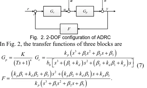
Fig. 2. 2-DOF configuration of ADRC In Fig. 2, the transfer functions of three blocks are



















 







3 2

1 2 3

3 2

0 1 2 1

2

1 2 3 2 3 3

3 2

1 2 3

1

. p

p n c

d d p

p d p d p

p

k s s s

K

G G

Ts b s k s k k s

k k s k k s k

F

k s s s

  

  

     

  

  

 

 

 _      _

    



  

(7)

[image:3.612.324.565.553.697.2]

 



 



 





 

2

1 2 3 2 3 3

3 2

0 1 2 1 1

p d p d p

l p c n

d d p

k k s k k s k _K

G s G G F

Ts

b s k s k k s

                          (8)

 

 

 



 

 









 



 



 

0 3 2

1 2 1

2

1 2 3 2 3 3

3 2

1 2 3

1 1

p c p

cl n

p c

d d p

p d p d p

G G k C s K

G s

G G F b A s Ts KB s

A s s k s k k s

B s k k s k k s k

C s s s s

                                 (9)

Thus, the frequency characteristic of the open loop transfer function..is

 

     





2

3 1 2 3 2 3

2 3

1 2 1 0

( ) ( )

.

( ) ( ) 1

l c p

p p d p d

n

d d p

G i G i G i F i

k k k k k i K

k k k i b T i

[image:4.612.95.247.297.428.2]

                              _    _  (10)

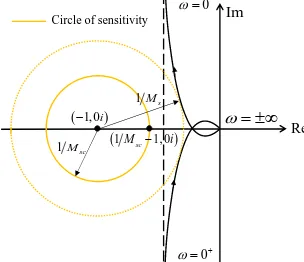
Figure 3 shows the Nyquist diagram ofG i_l

 

. Combined with equation (6), the definition of the maximum sensitivityM_s can be graphically interpreted: M_s equals to the inverse of the shortest distance between the Nyquist curve ofG i_l

 

and the critical point (-1,0i).

1, 0i

1Msc

Circle of sensitivity

Re

0

_ 

 

1Msc1, 0i

Im

0

_ 

1Ms

Fig. 3. Graphical interpretation of maximum sensitivity Ms

Given a certain maximum sensitivity constraintM_sc, a circle of sensitivity, centered at (-1,0i) with the radius1Msc, can be

constructed. Then the actual value of the maximum sensitivity

s

M is guaranteed to be not higher thanM_sc, provided that the Nyquist curve ofG il

 

does not enter into the circle of

sensitivity. This important principle will be used in next subsection to derive ADRC parameters tuning rules.

B. Derivation of ADRC tuning rule

As it is mentioned in Section II, _cis called the desired closed-loop bandwidth, also, the desired closed-loop system poles. When the observer gains are properly chosen so that the ESO states z z₁, ₂ and z₃ track

y y

,

and f well, combining equations (3), (4), the second equation in (1) can be rewritten as









0 0 . p d p d

k r y k y f

y f b k r y k y b

   

 

     (11)

Therefore, the transfer function from the reference

r

to the output y can be approximated into

 

_{ }

 





2

2 2.

p c

yr

d p c

k R s

G s

Y s s k s k s

 

  

   (12)

The choice of_c mainly influences the set-point tracking performance. In [24], it is recommended that *

10

c ts

  , where

* s

t is the desired settling time. The choice of the desired settling

time * s

t can incorporate the information of the process model. In this study, the controlled process,K



Ts1



n, can be seen as n

first-order processes 1



Ts1



being cascaded connecting together. Since parameters n and T influence the transient time of the process most, it is natural to assume that *

s

t is proportional tonT. Therefore, _cis decided as

10 ,

c knT

  (13)

where kis the desired settling time factor and it is the only tuning parameter in this proposed tuning method.

Bandwidth_ois the ESO pole. In general, a larger_ovalue can speed up the total disturbance being estimated and rejected, so a large_ois usually preferred. However, in practice, the sampling rate limits the upper bound of_o. In general, it is recommended that [23]

10 .

o c

   (14)

The tuning equation of _cis derived from the perspective of the desired set-point tracking, and the choice of_oconsiders the disturbance rejection speed. Now, the design ofb₀will consider the closed-loop system robustness, that is, sensitivity constraint will be applied in determination ofb₀.

Using the bandwidth-parameterization (5) and equation (14), the frequency characteristics of the open loop system transfer functionG il

 

, equation (10), can be rewritten as

 













2 _{3 3}

2 2

0

1.63 2.3 _{1 10}

.

32 361 1

c c _c

l n

c c

i _K

G i

b i T i

    _



    

 

 

    (15)

When come to derive PID control parameters under the sensitivity constraints, previous studies [26][27] have made effort on solving the nonlinear equations related to the definition of maximum sensitivity and the open loop transfer function.It is possible to yield explicit solutions for PID design, although derivation operation and numerical calculation are often involved, making it not easy for control engineers to execute the solving procedure. For the ADRC control system studied in this work, it is very difficult to directly solve the sensitivity constraint from equations (6) and (15). It is highly nonlinear because of the absolute operation. In addition, it is at least 5th-degree, which means it almost impossible to obtain an explicit solution.

Instead of strictly solving the sensitivity constraint, an alternative asymptote constraint is used to determine b0 in this

study. The asymptote is vertical to the real axis in the Nyquist plot of G il

 

(see Fig. 3). Considering the relationship

between the asymptote and the circle of sensitivity, an asymptote condition is further proposed below:

Provided that the vertical asymptote of Nyquist curve

 

l

G i is located at the right side of the circle of sensitivity, and the Nyquist curve of G il

 

does not enter into the circle

of sensitivity, then the actual maximum sensitivity M_s is guaranteed to be smaller thanM_sc.

The asymptote function of Nyquist curveG i_l

 

 needs to be found. Let x , y denote the real axis and imagine axis respectively, soG i_l

 

 x

 

 y

 

 i. The linexa is a vertical asymptote of the plot ofG i_l

 

 , when there exists a

 

 

 

 

* *

* *

lim lim Re

lim lim Im .

l

l

x G i a

y G i

                  _ _           (16)

Observed from Fig. 3, the imaginary coordinate of the Nyquist curve tends to infinity when



→ ±0, so the limiting values of the real and imaginary part ofG i_l

 

are concerned when



→ ±0. Let



1



1 2,

n

T i



p p i

   (17)

then

   

   

   

   

2 1 4 2

2 4

1

3 1 5 2

3 5

2

1 1 1

1 1 .

n n

n n

p C T C T

p nT C T C T

 

  

     

     

(18)

Therefore, we have

 



 



 





 





3 2 4 2 3

2

2 2 2

3 3

1 2

2 2

1 2 0

798.3 49.86 361 515.83 +1.63

32 361

10

.

c c c c

l

c c

c

i G i

p p i K

p p b

                      _{  }         (19) Then,  



 



 









3 2 4 2 3

1 2

2

2 2 2

3 3

2 2

1 2 0

798.3 49.86 361 515.83 +1.63

Re

32 361

10

c c c c

l c c c p p G i K

p p b

                      _{ }          (20)  





 









4

3 2 2 3

2 1

2

2 2 2

3 3

2 2

1 2 0

798.3 49.86 361 515.83 +1.63 Im

32 361

10 .

c

c c c

l c c c p p G i K p p b

                            _{ }          (21)

When



→0-_,

1 1

p  , p₂nT, and 2 2





2

1 2 1 1 1

n

p  p T i  , in the expressions of Re



G_l

 

i



andIm



G_l

 

i



, the terms in the form of multiplying



diminish to 0, while the terms which are divided by



tend to ∞. Thus, we have

 



 







 

3 4 3 3

2 4 0 0 2 3 0 0

798.3 361 10

lim Re

361 6.1256 2.77

lim Im .

c c _c

l c c c l nT K G i b nT K b G i                              (22)

As previously, when



→0+_,

 





 

2 3 0 0 0

lim Re 6.1256 2.77

lim Im - .

l c c

l

G i nT K b

G i                       (23)

Equations (22) and (23) show that there exists * 0satisfying the definition in (16), so the function of the asymptote is



2 3



0

6.1256 c 2.77 c .

x







nT K b (24) As it is shown in the Fig. 3, the right endpoint of the circle of sensitivity locates at



1M_sc1, 0i



. Applying the asymptote condition,



2 3



0

6.1256



_c 2.77



_cnT K b 1M_sc1, (25) and solving (25) forb₀, we have





2





0 2.77 c 6.1256 c sc sc 1

b  nT  K M M  (26)

Since increasingb₀can reduce the maximum sensitivityM_s, for a conservative design, letb₀be

m

times the lower limit. Then, the parameterb₀ can be determined by





2





0 2.77 c 6.1256 c sc sc 1 .

b m nT  K M M  (27) Coefficient

m

and M_sc can be chosen according to engineering experience. In this study, we choosem1.4, and the maximum sensitivity constraint M_sc is chosen as the maximum of the allowable value, 2.5, thus (27) becomes





2

0 6.4541 c 14.2726 c .

b  nT  K (28)

In summary, the tuning rules for the second-order linear ADRC controlling high-order processes K Ts



1



n are as follow:





2

0 10 10

6.4541 14.2726 .

c

o c

c c

knT

b nT K

              (29)

Similarly, the tuning rules for the first-order linear ADRC can also be derived.





2

0 10 10 11.1111 12.8042 c o c c c knT

b nT K

              (30)

Remark: Applying the proposed second-order ADRC tuning method to the high-order process, two interesting conclusions can be further inferred.

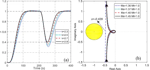
1) The asymptotes for the different controlled systems are the same. Substitute the expression ofb₀, equation (28), into the asymptote function (24), then we get x = -0.429. It shows the real axis value of the asymptote remains constant, which can be verified in the Fig. 4(b). Different Nyquist curves ofG il

 

converge to the same asymptote.

2) Complementary maximum sensitivityMt 1.

Complementary maximum sensitivity M_t is also an important indicator for measuring robustness. It implies the sensitivity of the closed-loop system to the large process dynamic variations.M_tis defined as

 



 







= max 1 , .

t l l

M G i G i











   (31)

SinceG i_l

     



x



y



i,

 

 

   

 

2 2

2 2

= max ,

1 2

t

x y M

x x y



 

  



   (32)

if x

 



 0.5, Mt 1. The proposed ADRC tuning

method gives asymptote functionx 0.429. Under the proposed tuning method, the Nyquist curve ofG i_l

 

 can be tuned to be located at the right side of the asymptote line, that is, x

 

 is not smaller than -0.429. Therefore, Mt1

is achieved. This conclusion indicates that the proposed ADRC tuning method derived underM_sconstraint can lead to satisfactoryM_t.

C. Tuning parameter

The effect of the tuning parameterk should be clear to users. According to [28], to ensure the closed loop system stability,

0

output response caused by nearing the critical values, the range of the tuning parameter k can be further narrowed. In engineering practice, the range of k1.0 ~ 4.0 is suitable for most high-order process. However, the adjustment ofkis still necessary to achieve a certain robustness level. Consider a cascaded fifth-order process





5

1 8 1 .

p

G  s (33)

The model parametern5,T8, andK1can be directly used to calculate the ADRC parameters by (29). The control results and robustness indices under the different tuning parameterkare shown in Fig. 4. In general, increasingkresults in faster tracking response and better disturbance rejection performance, but higher maximum sensitivity M_s . This influence pattern can be used as a crude guideline to adjust k to a certain maximum sensitivityM_s.

(a) (b)

Fig. 4. Performance and robustness under different tuning parameter k. (a) tracking response (t=0-200 s) and disturbance rejection (t=200-400 s)

of Gp; (b) Nyquist diagram and robustness indices of Gp.

Although this study provides a simple straightforward tuning method for ADRC parameters, sometimes it is better to give the values of parameters in the form of limitations. If a range of the tuning parameter k is decided, then the ADRC parameters can be presented in the form of limitations. For example, if an appropriate range of k is tuned for a certain process,

,

k k k_, then the ranges of ADRC parameters are

3 2 2 2 3 2 2 2

10 10

,

100 100

, .

6454.1 1427.26 6454.1 1427.26

, c

o

o

k nT k nT

k nT k nT

K K

b

k k n T k k n T





 

 

   

 _{ }



 _{ }

 



 _ 

 _{ }

 



 _{    }

 _  _{ }  _{ }

   

  



(34)

Theorem 1: Assuming the process is modelled by



1



n

K Ts , and the second-order ADRC is given by (2)~(4). ADRC parameters  _c, _oandb₀are controller parameters that need to be determined. Then, we have the following results: i) There exists an asymptote of the Nyquist curve of the

open-loop transfer function (8), which can be described by (24).

ii) If the asymptote is located at the right side of the circle of sensitivity, which is constructed by maximum sensitivity constraintM_sc. Thenb₀satisfies the inequality (26) andb₀ can bemtimes the lower limit, i.e.,b₀can be given by the equality (27).

iii) ADRC parameters _c, _oare given by (13) and (14), where the only tuning parameter k satisfies 0 k 4.5, so that ADRC can be tuned to achieve satisfactory performance

and robustness.

Remark 1:mandM_scin the Theorem can be determined by engineering experience. In this study, we choose m1.4,

2.5 sc

M  , then c, oandb0can be given by (29).

Remark 2:Similarly, when the controller is first-order ADRC, the controller parameters c, oandb0can be given by (30), where the only tuning parameterksatisfies 0 k 8.6.

Remark 3: For self-regulatory processes which can be approximated intoK Ts



1



n, the ADRC tuning equations (29) and (30) can also be applied.

IV. ILLUSTRATIVE EXAMPLES

In order to demonstrate the efficacy of the proposed ADRC tuning method, comparative simulation studies have been carried out for different types of processes.

A. Approximation method

Although the proposed ADRC tuning method is originally designed for the certain type of high-order processes,



1



n

K Ts , the proposed ADRC tuning method can also be applied to other types of processes, which can be approximated into the form of K Ts



1



n. The empirical two-point method is used for model approximation or process identification [29]. The principle of the two-point approximation is illustrated in Fig. 5 and (35). If the open-loop system step response indicates that the process is self-regulating, find the time coordinates t1, t2

corresponding to 0.4y(∞) and 0.8y(∞). Whent t_{1 2}0.46the process can be approximated to the high order process . Applying the empirical formulas (35), the model parameters

,

n TandKcan therefore be determined. It should be pointed out that the ordernshould be rounded to an integer in the calculation.

 







 



2

1 2 1

1 2

1.075 0.5

2.16

K y u n t t t T t t n

 



 _{   }

  

 _{ }



(35)

 

y

 

0.8y

 

0.4y

1

t t2

u

[image:6.612.53.295.243.356.2]

t

Fig. 5. Two-point approximation method B. Simulation examples

Example 1: 100th_{-order process}





100

1 1 1

p

G  s (36)

This is an extreme case of a standardK Ts



1



n - type high-order process. The model parameters n=100, T=1, and

K=1 can be directly used for ADRC parameters calculation. The well-known Skogestad IMC (SIMC) [30] and the

Ms-constrained integral gain optimization (MIGO) [26] design

instead of the simpler tuning rule AMIGO [31] is used in the simulations because the AMIGO does not have a tuning parameter to achieve a desired maximum sensitivity. Therefore, the tracking performance, disturbance rejection ability, and the control effort of different tuning methods can be compared under the same robustness level. The output responses with a unit load disturbance added to the system att800 s are depicted in Fig. 6(a). The simulation step size ish0.01. For the three simulations, white noises with a variance of 0.005 are added during the last one third of the simulation time span t_E. The parameters setting and performance indices are summarized in Table 1, including robustness indicesM_s,M_t, output performance settling timeT_s, overshoot , variance of control input noise_n, the integrated time-weighted absolute error (ITAE), and the control effort index total variation (TV) of the input. Indices ITAE and TV are defined in (37). They should be as small as possible [30].

   

2 1 3 2 3

1 0

1

ITAE d TV

E E

t h t

i i

i

t r t y t t u u



 



_

 



 (37)

It can be seen from the comparative results that under the same robustness levelMs1.51, the proposed ADRC tuning

rule provides smooth and non-overshoot tracking, meanwhile, gives better performance in disturbance rejection among these three control design methods. Moreover, it handles measurement well without additional filer. This 100th_-order

process behaves like systems with large time-delay. The success of controlling this model implies the possibility of applying this tuning method to other delay-dominate processes.

Example 2: Oscillatory high-order process













2 2 4

9 1

.

1 2 9 0.2755 1

p

G

s s s s

 

    (38)

This is a non-K Ts



1



n-type high-order process. G_p2can be approximated to a fourth-order process by using equations (35) of the two-point approximation method. Although the approximated high-order process cannot capture the oscillatory feature of the original process, the ability of ADRC estimating and compensating the un-modelled dynamics enables high-order process based ADRC design to provide good control results on oscillatory process. The proposed tuning equations (29) can be used to decide ADRC parameters. For SIMC-PID tuning, processG_p2is approximated to a second-order plus time delay process, 0.34s





0.72 1 0.14



1





e s s . ADRC,

SIMC-PID and MIGO are tuned to have the same maximum sensitivity, which isMs1.86. The detailed parameter settings

and the control results are show in Table I and Fig. 6(b). It can be seen from the Fig. 6(b) and Table 1 that the proposed ADRC tuning method provides least-oscillatory tracking performance with small overshoot, and the noise level under ADRC control is acceptable.

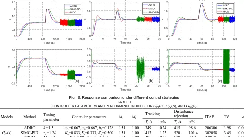
(a) (b) (c)

 

1

p

G s Gp2 s Gp3 s

[image:7.612.55.549.376.654.2]

(b) (a)

Fig. 6. Response comparison under different control strategies TABLE I

CONTROLLER PARAMETERS AND PERFORMANCE INDICES FOR GP1(S),GP2(S), AND GP3(S)

Models Method Tuning

parameter Controller parameters Ms Mt

Tracking Disturbance

rejection _{ITAE TV σn}

Ts /s σ/% Ts /s σ/%

Gp1(s)

ADRC k =1.5 ɷc=0.067, ɷo=0.667, b0=0.128 1.51 1.00 349 0.24 415 98.6 206306 1.98 0.0003

SIMC-PID τc =1.2θ Kp=0.833, Ki=0.333, Kd=0.500 1.51 1.00 413 1.23 520 101.4 302058 3.45 0.0076

MIGO Ms =1.5 K=0.2406, Ki=0.204,b=1 1.51 1.00 496 0.25 578 99.9 239575 1.76 0.0003

Gp2(s)

ADRC k =3.34 ɷc=2.717, ɷo=27.17, b0=37.34 1.86 1.08 4.41 3.38 4.65 47.5 13.8 2.64 0.0021

SIMC-PID τc =1.35θ Kp=1.069, Ki=1.242, Kd=0.124 1.86 1.03 5.83 6.43 4.88 53.3 15.5 15.0 1.0052

MIGO Ms =1.86 K=0.456, Ki=1.414,b=0 1.86 1.29 6.13 22.0 5.16 64.5 19.9 3.58 0.0008

Gp3(s)

ADRC k =2.55 ɷc=0.509, ɷo=5.088, b0=2.86 1.80 1.00 19.3 0.11 21.6 90.2 651 2.12 0.0016

SIMC-PID τc =0.6θ Kp=0.284, Ki=0.114, Kd=0.171 1.80 1.11 31.6 14.0 39.3 92.6 951 36.5 4.7022

Example 3: Process with time delay, non-minimum phase and high order













2

3 5 13

1 1

1 0.5929 1

s

p

s e G

s s

  

 

  (39)

As previously, processG_p3is approximated to a 13th_-order

process. Then, the proposed ADRC tuning method is applied and the SIMC-PID and MIGO are also performed for comparison. The comparative results in Fig. 6(c) and Table I show that the proposed ADRC tuning method delivers smooth and non-overshoot set-point tracking performance, better performance in disturbance rejection, while it requires least TV in control input.

Three illustrative examples have shown that the proposed ADRC tuning method is capable of providing good performance for cascade high-order process, non-cascade high-order process, time-delay process and non-minimum phase process. More simulation results can be found in

Supplementary materials.

Discussion:

The application scope of the proposed ADRC tuning method should be discussed. Generally speaking, the proposed tuning method is applicable to processes that can be modelled as or approximated to the form ofK Ts



1



n. The process must be self-regulatory, so processes with unstable or integrating characteristics are beyond the scope of this study. Processes with delay, oscillatory and non-minimum phase characteristics are target processes for the proposed tuning method. To be more specific, based on extensive simulations, delay-dominated systems, whose delay-lag constant ratio

1

T

  , are highly likely to be approximated toK Ts



1



n . Oscillatory systems with the damping ratio not smaller than 0.3, and non-minimum phase system with inverse overshoot not exceeding 30% of the steady-state gain are also recommended for this proposed tuning method. Since most of the industrial processes are self-regulatory, and many processes can be modelled into this high-order form, such as the steam temperature and pressure control, combustion control system in power plant, we believe that the proposed method is of certain generality and practical value.

The proposed tuning method requires the value of model parametersK n T, , , but this does not mean the proposed ADRC tuning laws depend on the exact modelling of the actual processes. Simulation examples ofG_p2andG_p3show that a rough approximation to the original process is enough for ADRC design. In addition, when a process is identified or approximated to aK Ts



1



n-type model, different choices of the model order n do not influence the control results notably. For instance, when the 100th_{-order process}

1

p

G , is modelled with different ordern , such asn102,98, 70, the control results based on these models with different n are very similar. This is because the ADRC has the ability of rejecting a total disturbance that includes the modelling errors. Besides, the ADRC tuning equations (29) and (30) do not solely depend on the model ordern, instead, it depend onnT together. This implies that when a process is modelled with differentn, the value nT may not change significantly, considering that a

highernusually results in a smallerTduring identification, and vice versa. Thus, controller parameters and control results remain similar.

The above simulations also show the influence of measurement noise on the control input for three different control strategies. For ADRC control system, no additional filter is added but the variance of the noise on control input is still at acceptable level. This can be explained by analysing the transfer function from the noises n to the control input u, Gun(s).

 





















2

2 1 0

3 2 2

0 1 0 2 1 0

0 3 1 2 3 2 1 2 3

0 2 1 1 1

1

1

1

, ,

, c un

c p

n

n

p p d p d

d p d

G F

G s

G FG

B s B s B Ts

b s A s A s Ts B s B s B K

B k B k k B k k

A k k A k

     

  

 

  



     

     

    

(40)

The Gun(s) is strictly proper, implying thatlim_Gun

 

i 0.

Therefore, the high-frequency component of the measurement noise will decay and make limited influence on the control input. For MIGO tuning, the derivative term is not used, so the noise has little influence on the control input. While for PID control system, Gun,PID(s) is not proper, so the high frequency

component of the noise will be magnified. Additional filter is necessary when high-frequency noise exists.

V. EXPERIMENTAL VERIFICATION AND FIELD TEST

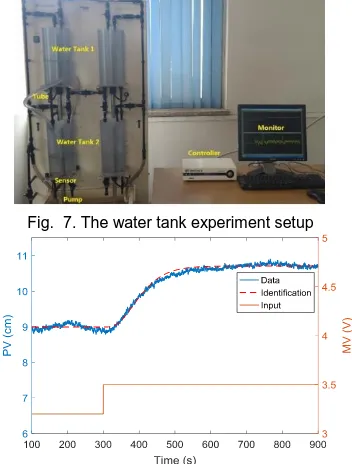
D. Experimental tests on water tank

To validate the proposed ADRC tuning method, a laboratory test is performed on a water tank system. Fig. 7 shows the experiment setup. The water tank control system, developed by ©Feedback Instruments Ltd, consists of water tanks, pumps, sensors, a controller, and a monitor. In this experiment, water tanks 1 and 2 connected by a water tube are used. Water level y

[image:8.612.354.530.496.728.2]

of Tank 2 is the process variable (PV), and the voltage of the pump u is the manipulated variable (MV).

Fig. 7. The water tank experiment setup

response

A step input is added in the open loop control system at the working point y =9 cm, as shown in Fig. 8. Noted that the water level y is slightly oscillatory before a step input is added, but this does not influence the design of control system because the proposed ADRC tuning does not relay on accurate modelling. A rough high-order model is identified from the open loop system response data by using the empirical equations (35).





4

5.72 27.72 1

G

s



 (41)

For comparison purpose, PID algorithm is also implemented on the water tank. PID controller is tuned by the SIMC method due to its simplicity in use. The choice of_c leads to the maximum sensitivity Ms1.4 and the PID controller

parameters areK_p 0.1458, Ki0.0021, Kd2.4249. The

tuning parameter of ADRC, the desired settling factork4.17, is manually tuned to achieve the same maximum sensitivity of SIMC-PID, which gives the controller parameters c 0.0278,

0.2775, o

  b₀0.0246.

These two controllers were tested by changing the water level set point from 9 cm to 11 cm first, then an input step disturbance d=1V is artificially added in the system at time t

=1000 s. Fig. 9 shows the real time control results. It can be seen that the proposed ADRC tuning results in slightly slower response during the set-point tracking, t= 500-1000 s, but ADRC has much better performance in disturbance rejection.

[image:9.612.133.486.374.524.2]

Moreover, the MV chattering under ADRC algorithm is less severe than SIMC-PID. Note that the calculated ADRC parameters are directly used on the plant without retuning. The experimental results demonstrate the reliability and effectiveness of the proposed ADRC tuning method.

Fig. 9. Experiment results under SIMC-PID and proposed ADRC tuning parameters

Although it is expected that ADRC behaves better than SIMC-PID in terms of disturbance rejection, the ADRC results of the water tank experiment show much better disturbance rejection than the simulated situation. A possible reason is that the working condition has varied, such as water level change of the water reserve, change of pump characteristic, to the direction that is beneficial to ADRC control.

2nd _{Desuperheater}

1st _{Desuperheater}

Steam drum

M/A M/A

Low temperature

superheater High temperature _superheater Desuperheater outlet temperature

Superheater steam temperature (SST)

T1 T2

Inner loop Controller

Outer loop Controller

Reference

From feed water

Steam

platen superheater

To turbine Spray water

valve Spray water

valve

Cascade control system

Flue gas Flue gas

Flue gas

Fig. 10. The schematic diagram of the superheater steam temperature control system in CFB power plant

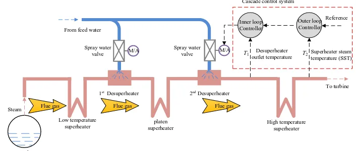
E. Field tests on a power plant

Encouraged by the positive results from simulation examples and water tank experiment, the proposed ADRC tuning method is further applied to the superheater steam temperature (SST) control in a 330 MW in-service CFB unit in Shanxi, China. The SST control system, which is one of the most important control systems in the power plant, is a typical high-order process. The SST has to be controlled within a certain range, so that the temperature will not exceed the upper limit that is set for safe operation of the steam turbine. At the meantime, the temperature will not drop out of the lower limit that ensures the efficiency of the whole power plant. For this CFB unit, the allowable SST temperature fluctuation range is ±5°C. The steam that comes from the drum is heated by the fuel gas through three sets of superheaters as show in Fig. 10. Two sets

of desuperheaters are deployed to control the steam temperature. Since the control of the 2nd _{desuperheater directly}

influence the SST, ADRC control algorithm and the proposed tuning method are implemented on the 2nd _{desuperheater.}

For the purpose of controller design, the SST models are identified from the open-loop data. As shown in Fig. 11, it is not a standard open-loop step test, because there is a spike in the control input signal and the control input changes before the temperature reaches steady state due to the operation limit. Therefore, the superheater models are identified by using optimization method instead of the empirical formulas presented in (35). The dynamic from the spray water valve to the desuperheater outlet temperatureT₁is denoted as model

 

1

[image:10.612.98.259.53.221.2]

Fig. 11. Identification results of the superheater steam temperature control system

The model identification process is accomplished by MATLAB Simulink parameter estimation tool. The chosen optimization method is pattern search. The model order

n

is decided by choosing the identified model with the lowest cost function value. The identification results are shown in Fig. 11 and the identified transfer functions are

 





 





1 2 2 4

1.6165 1.5528

.

19.363 1 28.234 1

G s G s

s s



 

  (42)

For the simplicity of implementing the control algorithm and relevant protective logics in the distributed control system (DCS), the first-order ADRC control algorithm is chosen to enhance the control performance of the SST control system. Compared to the outer loop process modelG₂

 

s , the inner loop process model G s₁

 

is relatively fast response, and usually the PI controller or even the P controller is enough to eliminate the disturbances in the inner loop. Therefore, the inner PI controller remains unchanged and the first-order ADRC is implemented as outer loop controller in parallel with the original outer loop PID controller (see Fig. 12).

ADRC

-up PI

-ua

r

Desuperheater valve position SST Reference

  2

G s

T2

  1 G s

T1

PI _u

-Desuperheater outlet tempreture SST

 

[image:10.612.326.549.125.418.2]

G s

Fig. 12. Cascade control system of the superheater steam temperature The tuning of the outer loop controller is based on the equivalent model G s

 

for the combined inner controlled system and the modelG₂

 

s , as shown in Fig. 12. The inner PI controller parameters are K_p2 1, K_i2 1 40 , so the equivalent model for outer loop controller is

 

   

_{      }



, 1

2 5

, 1

1.5528 .

1 27.4259 1

c inner

c inner

G s G s

G s G s

G s G s s

 

  (43)

The outer loop PI is tuned by the experienced field engineer, and the PI parameters areK_p11 3, Ki₁1 240, which results

in a robustness level ofMs1.5. ADRC controller parameters

are calculated by using (30). The desired settling time factor is manually tuned as k3.9 to achieve a similar maximum sensitivity of SIMC-PI tuning, which gives ADRC control parametersc 0.0187,o0.187,b₀0.4554.

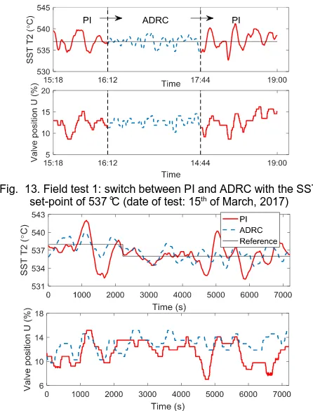
Two sets of field test results are shown in Fig. 13 and Fig. 14.

Fig. 13 shows the SST control result when the outer loop controller switches between PI and ADRC. Fig. 14 compares the control results under reference step change. It should be mentioned that the artificial input disturbance is not allowed for the commercial operation of the power plant, thus the strict disturbance rejection tests are not performed.

Fig. 13. Field test 1: switch between PI and ADRC with the SST set-point of 537°C (date of test: 15th _{of March, 2017)}

Fig. 14. Field test 2: SST set-point step from 538°C to 536°C (Time span of PI test: 14th _{of March, 2017 07:00-09:30; time span of ADRC test:}

16th _{of March, 2017 11:00-13:30)}

In addition, control performance indices such as peak positive errore, peak negative errore, standard deviation , integral absolute error (IAE) and the TV of control input, are summarized in Table II.

TABLEII

PERFORMANCE INDICES FOR THE SST CONTROL TESTS Test Controller e+_{/°C e}-_{/°C σ IAE TV}

Test 1 PID 4.20 -4.34 1.82 8519 44.4 ADRC 2.08 -2.59 1.05 4645 37.1

Test 2 PID 4.20 -5.63 1.93 9836 66.6 ADRC 2.18 -2.25 1.38 6757 53.5 It can be found that the proposed ADRC tuning method reduced the peak error and standard deviation



by about 50%. The IAE is reduced by more than 30%. The TV of the control input is decreased by about 20%, which means less overall tear and wear of valves, so the lifetime of valves can be prolonged and the maintenance cost is therefore reduced.

[image:10.612.55.282.472.536.2] [image:10.612.316.564.512.577.2]

VI. CONCLUSION

This paper describes the derivation of a quantitative tuning rule for low-order ADRC controller. In order to derive parameters under sensitivity constraint, an asymptote condition is propounded. Rooted from the high-order process system control, the proposed tuning rule has been expanded to other types of process applications. Comparative simulation studies, laboratory experiments and field tests have shown the efficiency of this tuning method. Future research will be continued on the ADRC parameters tuning toward multivariable processes.

REFERENCES

[1] H. Radim and R. Wagnerová, “Design and implementation of cascade control structure for superheated steam temperature control,” in Proc.

Carpathian Control Conference (ICCC), 2016 17th International. IEEE, pp. 253-258.

[2] L. Sun, et al., “Multi-objective optimization for advanced superheater steam temperature control in a 300 MW power plant,” Applied Energy, vol. 208, pp. 592-606, 2017.

[3] L. Sun, D. Li, K. Y. Lee and Y. Xue, “Control-oriented modeling and analysis of direct energy balance in coal-fired boiler-turbine unit,”

Control Engineering Practice, vol. 55, pp. 38-55, 2016.

[4] L. Peng, D. Chen and C. Wang, “A high-order model for spike-type instability in axial compression systems,” in Proc. 2017 36th _Chin.

Control Conf., July 2017, pp. 21811-2185.

[5] C. Ruth and K. Morris, “Transfer functions of distributed parameter systems: A tutorial,” Automatica, vol. 45.5, pp. 1101-1116, 2009. [6] L. Sun, D. Li, and K. Y. Lee, “Optimal disturbance rejection for PI

controller with constraints on relative delay margin,” ISA transactions, vol. 63, pp. 103-111, Jul. 2016.

[7] L. Guo and S. Cao, “Anti-disturbance control theory for systems with multiple disturbances: A survey,” ISA transactions, vol. 53, pp. 846-849, 2014.

[8] W. Chen, J. Yang, L. Guo and S. Li, “Disturbance-observer-based control and related methods—An overview,” IEEE Transactions on Industrial Electronics, vol. 63, pp. 1083-1095, 2016.

[9] J. Han, “Auto-disturbance rejection controller and its applications”,

Control and Decision, vol. 10, pp.85-88, 1998.

[10] J. Han, “From PID to active disturbance rejection control,” IEEE Transactions on Industrial Electronics, vol. 56, pp. 900-906, 2009. [11] H. Feng and B.Z. Guo, “Active disturbance rejection control: Old and

new results,” Annual Reviews in Control, vol. 44, pp. 226-237, 2017. [12] Z.L. Zhao and B.Z. Guo, “On convergence of nonlinear active

disturbance rejection control for a class of nonlinear systems,” Journal of Dynamical and Control Systems, vol. 22, pp. 385-412, 2016.

[13] S. Shao and Z. Gao, “On the conditions of exponential stability in active disturbance rejection control based on singular perturbation analysis,”

International Journal of Control, vol. 90, pp. 2085-2097, 2017. [14] Y. Huang and W. Xue, “Active disturbance rejection control:

methodology and theoretical analysis,” ISA transactions, vol. 53, pp. 963-976, 2014.

[15] L. Wang, Q. Li, C. Tong and Y. Yin, “Overview of active disturbance rejection control for systems with time-delay,” Control Theory & Applications, vol. 30, pp. 1521-1533, 2013.

[16] L. Sun, D. Li, Z. Gao, Y. Zhao, and S. Zhao, “Combined feedforward and model-assisted active disturbance rejection control for non-minimum phase system,” ISA transactions, vol. 64, pp. 24-33, 2016.

[17] S.N. Pawar and B.M. Patre, “Modified reduced order observer based linear active disturbance rejection control for TITO systems,” ISA transactions, vol. 71, pp. 480-494, 2017.

[18] L. Sun, J. Dong, D. Li and K.Y. Lee, “A practical multivariable control approach based on inverted decoupling and decentralized active disturbance rejection control,” Industrial & Engineering Chemistry Research, vol. 55, no. 7, pp, 2008-2019, 2016.

[19] Y. Xia, M. Fu, C. Li, F. Pu and Y. Xu, “Active disturbance rejection control for active suspension system of tracked vehicles with gun,” IEEE Transactions on Industrial Electronics, vol. 65, no. 5, pp. 4051-4059, 2018.

[20] Y. Su, C. Zheng and B. Duan, “Automatic disturbances rejection controller for precise motion control of permanent-magnet synchronous

motors,” IEEE Transactions on Industrial Electronics, vol. 52, no. 3, pp. 814-823, 2005.

[21] Q. Zheng and Z. Gao, “An energy saving, factory-validated disturbance decoupling control design for extrusion processes,” in Intelligent Control and Automation (WCICA), 2012 10th World Congress on, IEEE, pp. 2891-2896.

[22] S. Chen, Y. Zhang, D. Li and D. Lao, “ADRC decoupling controller design and parameters optimization for circulating fluidized bed boiler combustion system,” in Proc. 2013 32nd _{Chin. Control Conf., Xi’an,}

China, 2013, pp. 5504-5508. (in Chinese)

[23] Z. Gao, “Scaling and bandwidth-parameterization based controller tuning,” in Proceedings of the American control conference, vol. 6. pp. 4989-4996, 2006.

[24] X. Chen, D. Li, Z. Gao and C. Wang, “Tuning method for second-order active disturbance rejection control,” in Proc. 2011 30th_{Chin. Control}

Conf., Yantai, China, 2011, pp. 6322-6327.

[25] L. Wang, et al., “On control design and tuning for first order plus time delay plants with significant uncertainties,” in Proc. American Control Conference, Chicago, USA, 2015. pp. 5276-5281.

[26] K.J. Åström, H. Panagopoulos and T. Hägglund, “Design of PI controllers based on non-convex optimization,” Automatica, vol. 34, no. 5, pp. 585-601, 1998.

[27] Yaniv, O., and Nagurka, M., “Design of PID controllers satisfying gain margin and sensitivity constraints on a set of plants.” Automatica, vol. 40, pp. 111-116, 2004.

[28] C. Zhao and Y. Huang, “ADRC based input disturbance rejection for minimum-phase plants with unknown orders and/or uncertain relative degrees,” Journal of Systems Science and Complexity, vol. 25, no. 4, pp. 625-640, 2012.

[29] X. Yang, Automatic control for thermal process, 2nd ed., China: Tsinghua University Press, 2008. (in Chinese)

[30] S. Skogestad, “Simple analytic rules for model reduction and PID controller tuning,” Journal of process control, vol. 13, no. 4, pp. 291-309, 2003.

[31] T. Hägglund and K.J. Åström, “Revisiting the Ziegle-Nichols tuning rules for PI control,” Asian Journal of Control, vol. 4, no. 4, pp. 364-380, 2002. Ting He received her B.S. degree in the School of Aerospace Engineering, Beijing Institute of Technology, in 2014. She is currently working on the Ph.D. degree in the Department of Energy and Power Engineering, Tsinghua University. Her research interests include active disturbance rejection control, process control, distributed energy system modelling, simulation and control.

Zhenlong Wureceived the Bachelor’s degree in thermal and power engineering from the School of Energy and Environment, Southeast University, Nanjing, China, in 2015.He is currently working toward the Ph.D. degree in the Department of Energy and Power Engineering, Tsinghua University, Beijing, China. He has authored several publications in the field of active disturbance rejection control and process control.

Donghai Li received his Ph.D. degree from Tsinghua University, Beijing, China, in 1994. He is currently an Associate Professor with the Department of Energy and Power Engineering, Tsinghua University. He has published more than 110 papers in control science, chaired or participated in more than 20 research projects. His research interests are PID control, active disturbance rejection control, hydrogenerator control, and gasifier control.