https://doi.org/10.1007/s11222-019-09890-0
Multi-level Monte Carlo methods for the approximation of invariant
measures of stochastic differential equations
Michael B. Giles1·Mateusz B. Majka2·Lukasz Szpruch3·Sebastian J. Vollmer2·Konstantinos C. Zygalakis3
Received: 18 February 2019 / Accepted: 13 August 2019 © The Author(s) 2019
Abstract
We develop a framework that allows the use of the multi-level Monte Carlo (MLMC) methodology (Giles in Acta Numer. 24:259–328, 2015.https://doi.org/10.1017/S096249291500001X) to calculate expectations with respect to the invariant mea-sure of an ergodic SDE. In that context, we study the (over-damped) Langevin equations with a strongly concave potential. We show that when appropriate contracting couplings for the numerical integrators are available, one can obtain a uniform-in-time estimate of the MLMC variance in contrast to the majority of the results in the MLMC literature. As a consequence, a root mean square error ofO(ε)is achieved withO(ε−2)complexity on par with Markov Chain Monte Carlo (MCMC) methods,
which, however, can be computationally intensive when applied to large datasets. Finally, we present a multi-level version of the recently introduced stochastic gradient Langevin dynamics method (Welling and Teh, in: Proceedings of the 28th ICML, 2011) built for large datasets applications. We show that this is the first stochastic gradient MCMC method with complexity
O(ε−2|logε|3), in contrast to the complexityO(ε−3)of currently available methods. Numerical experiments confirm our
theoretical findings.
Keywords Numerical analysis·Monte Carlo methods·Stochastic Gradient methods
Mathematics Subject Classification62F15·65N75·65L20
1 Introduction
We consider a probability measure π(dx) with a density π(x)∝eU(x)onRdwith an unknown normalising constant. A typical task is the computation of the following quantity
B
Konstantinos C. Zygalakis [email protected]Michael B. Giles
Mateusz B. Majka
Lukasz Szpruch [email protected]
Sebastian J. Vollmer [email protected]
1 Mathematical Institute, University of Oxford, Oxford, UK
2 Department of Statistics, University of Warwick, Coventry,
UK
3 School of Mathematics, University of Edinburgh, Edinburgh,
UK
π(g):=Eπg=
Rd
g(x)π(dx), g ∈L1(π). (1)
Even ifπ(dx)is given in an explicit form, quadrature meth-ods, in general, are inefficient in high dimensions. On the other hand, probabilistic methods scale very well with the dimension and are often the method of choice. With this in mind, we explore the connection between dynamics of stochastic differential equations (SDEs)
dXt = ∇U(Xt)dt+
√
2dWt, X0∈Rd, (2)
and the target probability measure π(dx). The key idea is that under appropriate assumptions onU(x)one can show that the solution to (2) is ergodic and hasπ(dx)as its unique invariant measure (Has’minski˘ı1980). However, there exist only a limited number of cases where analytical solutions to (2) are available and typically some form of approximation needs to be employed.
analysis approach is that it might be the case that even though (2) is geometrically ergodic, the corresponding numerical discretisation might not be (Roberts and Tweedie 1996), while in addition extra care is required when∇Uis not glob-ally Lipschitz (Mattingly et al.2002; Talay2002; Roberts and Tweedie1996; Shardlow and Stuart2000; Hutzenthaler et al. 2011). The numerical analysis approach also introduces bias because the numerical invariant measure does not coincide with the exact one in general (Abdulle et al.2014; Talay and Tubaro1990), resulting hence in a biased estimation ofπ(g) in (1). Furthermore, if one uses the Euler–Maruyama method to discretise (2), then computational complexity1ofO(ε−3) is required for achieving a root mean square error of order
O(ε)in the approximation of (1). Furthermore, even if one mitigates the bias due to numerical discretisation by a series of decreasing time steps in combination with an appropriate weighted time average of the quantity of interest (Lamberton and Pagès2002), the computational complexity still remains
O(ε−3)(Teh et al.2016).
An alternative way of sampling fromπ(dx)exactly, so that it does not face the bias issue introduced by pure discretisa-tion of (2), is by using the Metropolis–Hastings algorithm (Hastings1970). We will refer to this as the computational statistics approach. The fact that the Metropolis Hastings algorithm leads to asymptotically unbiased samples of the probability measure is one of the reasons why it has been the method of choice in computational statistics. Moreover, unlike the numerical analysis approach, computational com-plexity ofO(ε−2)is now required for achieving root mean square error of orderO(ε)in the (asymptotically unbiased) approximation of (1). We notice that MLMC (Giles2015) and the unbiasing scheme (Rhee and Glynn 2012, 2015; Glynn and Rhee2014) are able to achieve theO(ε−2) com-plexity for computing expectations of SDEs on a fixed time interval [0,T], despite using biased numerical discretisa-tions. We are interested in extending this approach to the case of ergodic SDEs on the time interval[0,∞); see also discussion in Giles (2015).
A particular application of (2) is when one is interested in approximating the posterior expectations for a Bayesian inference problem. More precisely, if for a fixed parameter xthe data{yi}i=1,...,N are i.i.d. with densitiesπ(yi|x), then
∇U(x)becomes
∇U(x)= ∇logπ0(x)+
N
i=1
∇logπ(yi|x), (3)
withπ0(x)being the prior distribution of x. When dealing
with problems where the number of data itemsN 1 is
1In this paper the computational complexity is measured in terms of
the expected number of random number generations and arithmetic operations.
large, both the standard numerical analysis and the MCMC approaches suffer due to the high computational cost associ-ated with calculating the likelihood terms∇logπ(yi|x)over each data itemyi. One way to circumvent this problem is the stochastic gradient Langevin dynamics algorithm (SGLD) introduced in Welling and Teh (2011), which replaces the sum of theNlikelihood terms by an appropriately reweighted sum ofs Nterms. This leads to the following recursion formula
xk+1=xk+h
∇logπ0(xk)+
N s
s
i=1
∇logπ(yτk i |xk)
+√2hξk (4)
whereξkis a standard Gaussian random variable onRdand
τk=(τk
1, . . . , τsk)is a random subset of[N] = {1, . . . ,N}, generated, for example, by sampling with or without replace-ment from[N]. Notice that this corresponds to a noisy Euler discretisation, which for fixed N,sstill has computational complexity O(ε−3)as discussed in Teh et al. (2016) and Vollmer et al. (2016). In this article, we are able to show that careful coupling between fine and coarse paths allows the application of the MLMC framework and hence reduc-tion of the computareduc-tional complexity of the algorithm to
O(ε−2|logε|3). We also remark that coupling in time has
been recently further developed in Fang and Giles (2016), Fang and Giles (2017) and Fang and Giles (2019) for Euler schemes.
We would like to stress that in our analysis of the com-putational complexity of MLMC for SGLD, we treatN and sas fixed parameters. Hence, our results show that in cases in which one is forced to considers N samples (e.g. in the big data regime, where the cost of taking into account allN samples is prohibitively large) MLMC for SGLD can indeed reduce the computational complexity in comparison with the standard MCMC. However, recently the authors of Nagapetyan et al. (2017) have argued that for the standard MCMC the gain in complexity of SGLD due to the decreased number of samples can be outweighed by the increase in the variance caused by subsampling. We believe that an analo-gous analysis for MLMC would be highly non-trivial and we leave it for future work.
In summary, the main contributions of this paper are:
1. Extension of the MLMC framework to the time interval
[0,∞)for (2) whenUis strongly concave.
2. A convergence theorem that allows the estimation of the MLMC variance using uniform-in-time estimates in the 2-Wasserstein metric for a variety of different numerical methods.
steps (as in MCMC). The methods we propose can be better parallelised than MCMC, since computations on all levels can be performed independently.
4. The application of this scheme to stochastic gradient Langevin dynamics (SGLD) which reduces the com-plexity ofO(ε−3)toO(ε−2|logε|3)much closer to the standardO(ε−2)complexity of MCMC.
The rest of the paper is organised as follows: In Sect.2we describe the standard MLMC framework, discuss the con-tracting properties of the true trajectories of (2) and describe an algorithm for applying MLMC with respect to timeT for the true solution of (2). In Sect.3 we present the new algorithm, as well as a framework that allows proving its convergence properties for a numerical method of choice. In Sect.4we present two examples of suitable numerical meth-ods, while in Sect.5we describe a new version of SGLD with complexityO(ε−2|logε|3). We conclude in Sect.6where a number of relevant numerical experiments are described.
2 Preliminaries
In Sect. 2.1 we review the classic, finite time, MLMC framework, while in Sect.2.2we state the key asymptotic properties of solutions of (2) whenU is strongly concave.
2.1 MLMC with fixed terminal time
Fix T > 0 and consider the problem of approximating E[g(XT)] where XT is a solution of the SDE (2) and
g:Rd →R. A classical approach to this problem consists of constructing a biased (bias arising due to time-discretisation) estimator of the form
1 N
N
i=1
gxTM(i), (5)
where (xTM)(i) for i = 1, . . . ,N are independent copies of the random variablexTM, with{xkhM}kM=0 being a discrete time approximation of (2) over[0,T]with the discretisa-tion parameterh and with M time steps, i.e.M h = T. A central limit theorem for the estimator (5) has been derived in Duffie and Glynn (1995), and it was shown that its com-putational complexity isO(ε−3), for the root mean square errorO(ε) (as opposed toO(ε−2)that can be obtained if we could sampleXT without the bias). The recently devel-oped MLMC approach allows recovering optimal complexity
O(ε−2), despite the fact that the estimator used therein builds
on biased samples. This is achieved by exploiting the follow-ing identity (Giles2015; Kebaier2005)
E[gL] =E[g0] +
L
=1
E[g−g−1], (6)
where g := g(xTM)and for any = 0. . .L the Markov chain {xkhM
}
M
k=0 is the discrete time approximation of (2)
over [0,T], with the discretisation parameter h and with Mtime steps ( henceMh =T). This identity leads to an unbiased estimator ofE[gL]given by
1 N0
N0
i=1 g0(i,0)+
L
=1
⎧ ⎨ ⎩
1 N
N
i=1
g(i,)−g(i−,)1
⎫ ⎬ ⎭,
where g(i,) = gxTM(i)andg(i−,)1 = g((xM−1 T )(i))are independent samples at level. The inclusion of the levelin the superscript(i, )indicates that independent samples are used at each level. The efficiency of MLMC lies in the cou-pling ofg(i,)andg(i−,)1 that results in small Var[g−g−1].
In particular, for the SDE (2) one can use the same Brownian path to simulategandg−1which, through the strong
con-vergence property of the underlying numerical scheme used, yields an estimate for Var[g−g−1].
By solving a constrained optimisation problem (cost and accuracy), one can see that reduced computational complex-ity (variance) arises since the MLMC method allows one to efficiently combine many simulations on low accuracy grids (at a corresponding low cost), with relatively few simulations computed with high accuracy and high cost on very fine grids. It is shown in Giles (2015) that under the assumptions2
E[g−g]| ≤c1hα
, Var[g−g−1] ≤c2hβ, (7)
for someα≥1/2, β >0,c1>0 andc2>0,the
computa-tional complexity of the resulting multi-level estimator with accuracyεis proportional to
C= ⎧ ⎪ ⎨ ⎪ ⎩
ε−2, β > γ,
ε−2log2(ε), β =γ, ε−2−(1−β)/α, 0< β < γ
where the cost of the algorithm is of orderh−Lγ. Typically, the constantsc1,c2grow exponentially in timeT as they
fol-low from classical finite time weak and strong convergence analysis of the numerical schemes. The aim of this paper is to establish the bounds (7) uniformly in time, i.e. to find constantsc1,c2>0 independent ofT such that
sup T>0
E[g−g]| ≤c1hα , sup
T>0
Var[g−g−1] ≤c2hβ.
(8)
2 Recallh
Remark 2.1 The reader may notice that in the regime when β > γ, the computationally complexity ofO(ε−2)coincides with that of an unbiased estimator. Nevertheless, the MLMC estimator as defined here is still biased, with the bias being controlled by the choice of final level parameterL. However, in this setting it is possible to eliminate the bias by a clever randomisation trick (Rhee and Glynn2015).
2.2 Properties of ergodic SDEs with strongly
concave drifts
Consider the SDE (2) and letUsatisfy the following condi-tion
HU0For anyx,y ∈Rd there exists a positive constant ms.t.
∇U(y)− ∇U(x),y−x ≤ −m|x−y|2, (9)
which is also known as a one-side Lipschitz condition. Con-ditionHU0 is satisfied for strongly concave potential, i.e. when for anyx,y∈Rdthere exists constantms.t.
U(y)≤U(x)+ ∇U(x),y−x − m 2|x−y|
2.
In additionHU0implies that
∇U(x),x ≤ −m 2|x|
2+ 1
2m|∇U(0)| 2, ∀
x ∈Rd (10)
which in turn implies that
∇U(x),x ≤ −m|x|2+2b|∇U(0)|2, ∀x∈Rd (11)
for some3m >0,b≥ 0. ConditionHU0ensures the con-traction needed to establish uniform-in-time estimates for the solutions of (2). For the transparency of the exposition we introduce the following flow notation for the solution to (2), starting atX0=x
ψs,t,W(x):=x+
t
s
∇U(Xr)dr+
t
s
√
2dWr, x∈Rd. (12)
The theorem below demonstrates that solutions to (2) driven by the same Brownian motion, but with different initial con-ditions, enjoy an exponential contraction property.
Theorem 2.2 Let(Wt)t≥0be a standard Brownian motion in
Rd. We fix random variables Y
0, X0∈Rd and define XT =
ψ0,T,W(X0)and YT =ψ0,T,W(Y0). IfHU0holds, then
3If∇U(0)=0 thenm=m,b=0. Otherwisem<m(implication
of Young’s inequality).
E|XT −YT|2≤E|X0−Y0|2e−2mT (13) Proof The result follows from Itô’s formula. Indeed, we have
1 2e
2mt|
Xt−Yt|2= 1
2|X0−Y0|
2+
t
0
me2ms|Xs−Ys|2ds
+ t
0
e2ms∇U(Xs)− ∇U(Ys),Xs−Ysds.
AssumptionHU0yields
E|XT −YT|2≤e−2mTE|X0−Y0|2,
as required.
Remark 2.3 The 2-Wasserstein distance between probability measuresν1andν2defined on a Polish metric spaceE, is
given by
W2(ν1, ν2)=
inf π∈(ν1,ν2)
E×E
|x−y|2π(dx,dy)
1 2
,
with(ν1, ν2)being the set of couplings ofν1andν2(all
probability measures onE×Ewith marginalsν1andν2). We
denoteL(ψ0,t,W(x))=Pt(x,·). That is,Pt is the transition kernel of the SDE (2). Since the choice of the same driving Brownian motion in Theorem2.2is an example of a coupling, Equation (13) implies
W2(Pt(x,·),Pt(y,·))≤ |x−y|exp(−mt) (14)
Consequently, Pt has a unique invariant measure, and thus, the process is ergodic (Hairer et al. 2011). In the present paper we are not concerned with determining couplings that are optimal; for practical considerations one should only consider couplings that are feasible to implement [see also discussion in Agapiou et al. (2018) and Giles and Szpruch (2014)].
2.3 Coupling in time
T
For the MLMC method with different discretisation param-eters on different levels, coupling with the same Brownian motion is not enough to obtain good upper bounds on the variance, as, in general, solutions to SDEs (2) are 1/2-Hölder continuous (Krylov2009), i.e. for anyt>s>0 there exists a constantC >0 such that
E|Xt−Xs|2≤C|t−s| (15)
solutions on time intervals of lengthTandS,T >S, respec-tively, we will be able to take advantage of the exponential contraction property obtained in Theorem2.2.
Let (T)≤0 be an increasing sequence of positive real
numbers. To couple processes with different terminal times TiandTj,i= j, we exploit the time homogeneous Markov property of the flow (12). More precisely, for each≥0 one would like to construct a pair(X(f,),X(c,))of solutions to (2), which we refer to as fine and coarse paths, such that
L(X(f,)(T
−1))=L(XT),
L(X(c,)(
T−1))=L(XT−1), ∀≥0, (16) and
E|X(f,)(T
−1)−X(c,)(T−1)|2≤E|XT−XT−1|
2. (17)
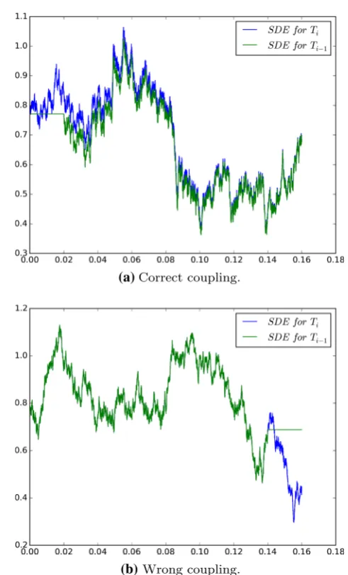
Following Rhee and Glynn (2012, 2015); Agapiou et al. (2018); Giles (2015), we propose a particular coupling denoted by(X(f,),X(c,)), and constructed in the follow-ing way (see also Fig.1a)
– First4obtain a solution to (2) over[0,T−T−1]. We fix
anRd-valued random variableX(0)and takeX(f,)(0)= ψ0,(T−T−1),W˜(X(0)).
– Next couple fine and coarse paths on the remaining time interval[0,T−1]using the same Brownian motion W,
i.e.
X(f,)(T−1)=ψ0,T−1,W(X(
f,)(0)),
and
X(c,)(T−1)=ψ0,T−1,W(X(0)).
We note here that∇U(·)in (2) is time homogenous; hence, the same applies for the corresponding transition kernel
L(ψ0,t,W(x))= Pt(x,·), which implies that condition (16) holds. Now Theorem2.2yields
E|X(f,)(T−1)−X(c,)(T−1)|2≤E|X(f,)(0)−X(0)|2e−2mT−1. (18) implying that condition (17) is also satisfied. We now take ρ >1 and define
T:= log 2
2m ρ(+1) ∀≥0. (19)
In our case g(i,) = g((X(f,)(T−1))(i)) and g(i−,)1 = g((X(c,)(T−1))(i))and we assume thatgis globally
Lips-chitz with LipsLips-chitz constantK. Hence,
4As we can see in Fig.1b, doing this first is important for the overall
difference of the paths.
(a) Correct coupling.
(b) Wrong coupling.
Fig. 1 Shifted couplings
E|g(X(f,)(T−1))−g(X(c,)(T−1))|2 ≤K2E|X(f,)(T−1)−X(c,)(T−1)|2 ≤K2E|X(f,)(0)−X(0)|2e−2mT−1
≤K2E|X(f,)(0)−X0|22−ρ ≤K2C|T−T−1|2−ρ. ∀i ≥0,
where the last inequality follows from (15).
3 MLMC in
T
for approximation of SDEs
[image:5.595.298.544.48.454.2]3.1 Description of the general algorithm
We now focus on the numerical discretisation of the Langevin equation (2). In particular, we are interested in coupling the discretisations of (2) based on step sizeh andh−1 with h=h02−. Furthermore, as we are interested in computing
expectations with respect to the invariant measureπ(dx), we also increase the time endpointT ↑ ∞which is chosen such thath0T,Th
∈N. We illustrate the main idea using two generic discrete time stochastic processes(xk)k∈N, (yk)k∈N which can be defined as
xk+1=Shf,ξk(xk), yk+1=S
c
h,ξ˜k(yk), (20)
where Sh,ξk(xk) = S(xk,h, ξk)and the operators S
f,Sc : Rd×R
+×Rd×m →Rdare Borel measurable, whereasξ,ξ˜ are random inputs to the algorithms. The operatorsSf and Scin (20) need not be the same. This extra flexibility allows analysing various coupling ideas.
For example, for the Euler discretisation we have
Sh,ξ(x)=x+h∇U(x)+
√
2hξ,
whereξ ∼N(0,I). We will also use the notationPh(x,·)=
LSh,ξ(x)
for the corresponding Markov kernel.
For MLMC algorithms one evolves both fine and coarse paths jointly, over a time interval of lengthT−1, by doing
two steps for the finer level (with the time steph) and one on the coarser level (with the time steph−1). We will use
the notation(x·f), (x·c)for
xf
k+12 =S f
h
2,ξk+1 2
xkf
, xkf+1=Shf
2,ξk+1
xf
k+12
(21)
xkc+1=Sc
h,ξ˜k+1
xkc. (22)
The algorithm generating(xkf)k∈N/2and(xkc)k∈Nis presented in Algorithm1.
3.2 General convergence analysis
We will now present a general theorem for estimating the bias and the variance in the MLMC set up. We refrain from pre-scribing the exact dynamics of(xk)k≥0and(yk)k≥0in (20),
as we seek general conditions allowing the construction of uniform-in-time approximations of (2) in theL2-Wasserstein norm. The advantage of working in this general setting is that if we wish to work with more advanced numerical schemes than the Euler method (e.g. implicit, projected, adapted or randomised scheme) or general noise terms (e.g. α-stable processes), it will be sufficient to verify relatively simple con-ditions to see the performance of the complete algorithm. To
1. Setx0(f,)=x0, then simulate according toPh(x0,·)up to
timeT−T−1
h , thus obtainingx (f,)
T−T−1 h
;
2. Setx0(c,)=x0andx0(f,)=x(
f,)
T−T−1 h
, then simulate
(x(·f,),x(·c,))jointly as
xk(+1f,),xk(c+1,)=Shf
,ξk+1◦S
f h,ξk+1
2
(xk(f,)),
Sc h−1,√12
ξk+1 2+ξk+1
(xk(c,)).
3. Setk:= T−1
h−1 and
(i)
:=g
xk(f,)
(i) −g
xk(c,)
(i)
Algorithm 1: Coupling Langevin discretisations for T↑ ∞.
give the reader some intuition behind the abstract assump-tions, we discuss the specific methods in Sect.4.
3.2.1 Uniform estimates in time
Definition 3.1 (Bias) We say that a process (xk)k∈N con-verges weakly uniformly in time with order α > 0 to the solution (Xt)t≥0 of the SDE (2), if there exists a constant c>0 such that for anyh>0,
sup t≥0|E[
g(Xt)] −E[g(xt/h)]| ≤chα g∈CrK(R).
We define MLMC variance as follows:
Definition 3.2 (MLMC variance) Let the operators in (21)– (22) satisfy that for allx
LShf,ξ(x)
=LSc
h,ξ˜(x)
. (23)
We say that the MLMC variance is of orderβ > 0 if there exists a constantcV >0 s.t. for anyh>0,
sup t≥0E|
g(xct/h)−g(x f t/h)|
2≤
cVhβ. (24)
3.2.2 Statement of sufficient conditions
We now discuss the necessary conditions imposed on a generic numerical method (20) to estimate MLMC variance. We decompose the global error into the one step error and the regularity of the scheme. To proceed we introduce the notationxkh,x
conditional expectation operator asEn[·] :=E[·|Fn], where
Fn:=σ
xkh:k≤n.
We now have the following definition.
Definition 3.3 (L2-regularity). We will say that the one step operatorS : Rd×R+×Rd×m → Rd isL2-regular uni-formly in timeif for anyFn-measurable random variables
xn,yn ∈ Rd there exist constantsK,CR,CH,β > 0 and random variablesZn+1,Rn+1 ∈ Fn+1andHn ∈ Fn, such that for allh∈(0,1)
Sh,ξn+1(xn)−Sh,ξn+1(yn)=xn−yn+Zn+1 and
En[|Sh,ξn+1(xn)−Sh,ξn+1(yn)|
2] ≤(1−K h)|x
n−yn|2
+Rn
En[|Zn+1|2] ≤Hn|xn−yn|2h, (25)
where
sup n≥1
E
n−1
i=0
e(i−(n−1))h K/2Ri
≤CRhβ,
sup n≥1
E|Hn|2
≤CH. (26)
We now introduce the set of the assumptions needed for the proof of the main convergence theorem.
Assumption 1 Consider two processes(xkf)2k∈Nand(xkc)k∈N obtained from the recursive application of the operators Shf,ξ(·)andShc,ξ(·)as defined in (20). We assume that
H0 There exists a constantH >0 such that for allq>1
sup k
E|xkf|q≤ H and sup k
E|xck|q≤ H.
H1 For anyx∈Rd
LShf,ξ(x)
=LSc
h,ξ˜(x)
.
H2 The operatorShf,ξ(·)isL2-regular uniformly in time. Below, we present the main convergence result of this section. By analogy to (21)–(22), we use the notation
xnf,xc n−1 =S
f h,ξn
xf
n−12,xnc−1
xf
n−12,xc n−1
=Shf,ξ n−1
2
xnc−1 xnc,xc
n−1 =S c h,ξ˜n
xnc−1
.
Using the estimates derived here, we can immediately esti-mate the rate of decay of MLMC variance.
Theorem 3.4 Take(xnf)n∈N/2and (xnc)n∈N with h ∈ (0,1]
and assume thatH0–H2hold. Moreover, assume that there exist constants cs >0,cw >0andα ≥ 12,β ≥ 0, p ≥ 1
withα≥ β2 such that for all n≥1
|En−1
xnc,xc n−1−x
f n,xnc−1
| ≤cw(1+ |xnc−1|p)hα+1, (27)
and
En−1
|xnc,xc
n−1−x f n,xnc−1|
2≤c
s(1+ |xnc−1|2p)hβ+1. (28) Then, the global error is bounded by
E[|xTc/h,x
0 −x f T/h,y0|
2] ≤ |x
0−y0|2e−K/2T +2hβ/K +
n−1
j=0
e(j−(n−1))h K/2E(Rj) ,
where T/h=n andis given by(29). Proof We begin using the following identity
xnc,x0 −x f
n,y0 =xnc,xc n−1−x
f n,xnf−1
=xnc,xc n−1−x
f n,xn−c 1
+xnf,xc n−1 −x
f n,xnf−1
.
We will be able to deal with the first term in the sum by using Equations (27) and (28), while the second term will be controlled because of the L2regularity of the numerical scheme. Indeed, by squaring both sides in the equality above, we have
|xnc,y0−x f
n,x0|2= |xcn,xc n−1−x
f n,xnc−1|
2 + |xnf,xc
n−1 −x f n,xn−f 1|
2 +2xnc,xc
n−1−x f n,xnc−1,x
c n−1−x
f n−1+Zn
,
where in the last line we have used AssumptionH2. Applying conditional expectation operator to both sides of the above equality, we obtain
En−1[|xnc,y0−x f
n,x0|2] =En−1
|xnc,xc
n−1−x f n,xnc−1|
2 +En−1
|xnf,xc
n−1−x f n,xn−f 1|
2 +2xnc−1−xnf−1,En−1
xnc,xc n−1−x
f n,xcn−1
+2En−1
Zn,xnc,xc n−1−x
f n,xc
n−1
Applying Cauchy–Schwarz inequality and using the weak error estimate (27) lead to
En−1
|xnc,y0 −xnf,x0|
2≤En
−1
|xnc,xc
n−1−x f n,xc
n−1|
2 +En−1
|xnf,xc
n−1−x f n,xnf−1|
2
+2cwhα+1|xnc−1−xnf−1|1+ |xnc−1|p
+2(En−1[|Zn|2])1/2
En−1[|xcn,xc n−1−x
f n,xnc−1|
2]1/2 .
By AssumptionsH0–H2and the strong error estimate (28), we have
En−1[|xcn,y 0−x
f n,x0|
2] ≤cs(1+ |xc
n−1|2p)hβ+1
+ |xnc−1−xnf−1|2(1−K h)+Rn−1
+2cwhα+1|xnc−1−xnf−1|(1+ |xnc−1|p)
+2
En−1[Hn]|xnc−1−x
f n−1|2h
1/2
cs(1+ |xnc−1|2p)hβ+1 1/2
≤cs(1+ |xnc−1|2p)hβ+1+ |xnc−1−xnf−1|2(1−K h)+Rn−1 +2cwhα+1|xnc−1−xnf−1|(1+ |xnc−1|p)
+2|xnc−1−xnf−1|2h1/2csEn−1Hn(1+ |xnc−1|2p)
hβ+11/2,
while taking expected values and applying Cauchy–Schwarz inequality and the fact thatα ≥ β2 andh < 1 (and hence hα+1≤hβ2+1) give
E[|xnc,y0−xnf,x0|
2] ≤cs(1+E[|xc
n−1|2p])hβ+1 +E[|xcn−1−xnf−1|2](1−K h)+E[Rn−1]
+2√2cwE|xnc−1−xnf−1|2h1/2E(1+ |xnc−1|2p)hβ+11/2
+2E|xnc−1−xnf−1|2h1/2EcsHn−11+ |xnc−1|2phβ+1
1/2
.
Now Young’s inequality gives that for anyε >0
E|xnc−1−xnf−1|2h1/2E1+ |xnc−1|2phβ+11/2
≤εExnc−1−xnf−12h+ 1 4εE
1+ |xnc−1|2phβ+1
and
E|xnc−1−xnf−1|2h1/2EcsHn−11+ |xnc−1|2phβ+1
1/2
≤εE|xcn−1−xnf−1|2h+ 1 4εE
csHn−1
1+ |xnc−1|2phβ+1,
while
EHn−11+ |xnc−1|2p≤
1 2E
|Hn−1|2
+E1+ |xnc−1|4p.
Letγn := E[|xnc,y0 −x f
n,x0|2]. Since(1+E[|xnc−1|2p]) ≤ (1+E[|xnc−1|4p]), we have
γn≤
csH+
2√2cwH+cs
E[|Hn−1|2] +2H
4ε
hβ+1
+E[Rn−1] +γn−1
1− [K−(2√2cw+2)ε]h
Fixε= K
2(2√2cw+2), and define
:=
csH+
2√2cw+2
×
2√2cwH+cs
E[supn|Hn−1|2] +2H
2K
. (29)
We have
γn≤(1−K h/2) γn−1+hβ+1+E[Rn−1]. (30)
We complete the proof by Lemma3.5.
Lemma 3.5 Let an,gn,c ≥ 0, n ∈ Nbe given. Moreover,
assume that1+λ >0. Then, if an∈R, n∈N, satisfies
an+1≤an(1+λ)+gn+c, n≥0,
then
an≤a0enλ+c enλ−1
λ +
n−1
j=0
gje((n−1)−j)λ, n ≥1.
Remark 3.6 Note that if we can chooseβ > β in (26) (which, as we will see in Sect.4, is the case, for example, for Euler and implicit Euler schemes), then from Theorem3.4we get
E[|xcT/h,x0−xTf/h,y
0|
2] ≤ |x
0−y0|2e−K/2T+(2/K+CR)hβ.
3.2.3 Optimal choice of parameters
Theorem3.4is fundamental in terms of applying the MLMC as it guarantees that the estimate for the variance in (7) holds. In particular, we have the following lemma.
Lemma 3.7 Assume that all the assumptions from Theorem
3.4hold. Let g(·)be a Lipschitz function. Define
h=2−, T ∼ −2β
K (logh0+log 2) , ∀≥0. Then, resulting MLMC variance is given by.
Var[] ≤2−β, =g
x(Tf−,)1 h−1
−g
x(Tc,)−1 h−1
Proof Sincegis a Lipschitz function and
ExhT−T−1 h
−x0
2 <∞,
the proof is a direct consequence of Theorem3.4. Remark 3.8 Unlike in the standard MLMC complexity theo-rem (Giles2015) where the cost of simulating single path is of orderO(h−1), here we haveO(h−1|logh|). This is due to the fact that terminal times are increasing with levels. For the case h = 2− this results in cost per path O(2−) and does not exactly fit the complexity theorem in Giles (2015). Clearly in the case when MLMC variance decays withβ >1, we still recover the optimal complexity of order
O(ε−2). However, in the caseβ = 1 following the proof
by Giles (2015), one can see that the complexity becomes
O(ε−2|logε|3).
Remark 3.9 In the proof above we have assumed thatK is independent ofh, while we have also used crude bounds in order not to deal directly with all the individual constants, since these would be dependent on the numerical schemes used.
Example 3.10 In the case of the Euler–Maruyama method as we see from the analysis5in Sect.4.1K =2m−L2h, β= 2, whileRn =0,Hn =L. HereL is the Lipschitz constant of the drift∇U(x).
4 Examples of suitable methods
In this section we present two (out of many) numerical schemes that fulfil the conditions of Theorem3.4. In particu-lar, we need to verify that our scheme isL2-regular in time, it has bounded numerical moments as inH0, and finally that it satisfies the one-step error estimates (27)–(28). Note that for both methods discussed in this section we verify condition (25) withh2instead ofh. However, since in (25) we consider h∈(0,1), both (35) and (42) imply (25).
4.1 Euler–Maruyama method
We start by considering the explicit Euler scheme
Shf,ξ(x)=x+h∇U(x)+√2hξ, (31)
while Sf = Sc, that is, we are using the same numerical method for the fine and coarse paths. In order to be able to recover the integrability and regularity conditions, we will
5As we will see therem≤mdepending on the size of∇U(0).
need to impose further assumptions on the potential6U. In particular, additionally to AssumptionHU0, we assume that
HU1 There exists constantL such that for anyx,y∈Rd
|∇U(x)− ∇U(y)| ≤L|x−y|
As a consequence of this assumption, we have
|∇U(x)| ≤L|x| + |∇U(0)| (32)
We can now prove theL2-regularity in time of the scheme. L2-regularitySince regularity is a property of the numer-ical scheme itself and it does not relate with the coupling between fine and coarse levels, for simplicity of notation we prove things directly for
xn+1,xn =S
f
h,ξn+1(xn). (33)
In particular, the following lemma holds.
Lemma 4.1 (L2-regularity)LetHU0andHU1hold. Then, the explicit Euler scheme is L2-regular, i.e.
En−1[|xn,xn−1−xn,yn−1|
2] ≤(1−(2m−L2h)h)|x
n−1−yn−1|2
(34)
En−1[|Zn|2] ≤h2L2|xn−1−yn−1|2 (35) Proof The difference between the Euler scheme taking val-uesxn−1andyn−1at timen−1 is given by
xn,xn−1 −xn,yn−1 =xn−1−yn−1
+h(∇U(xn−1)− ∇U(yn−1)).
This, along withHU0andHU1, leads to
En−1[(xn,xn−1 −xn,yn−1)
2] = |
xn−1−yn−1|2 +2h∇U(xn−1)− ∇U(yn−1),xn−1−yn−1 + |∇U(xn−1)− ∇U(yn−1)|2h2
≤ |yn−1−xn−1|2(1−2mh+L2h2) = |yn−1−xn−1|2(1−(2m−L2h)h).
This proves the first part of the lemma. Next, due toHU1
En−1[|Zn|2] =h2En−1[|∇U(xn−1)− ∇U(yn−1)|2] ≤h2L2|xn−1−yn−1|2.
6 This restriction will be alleviated in Sect.4.2by means of more
Integrability In the Lipschitz case we only require mean square integrability. This will become apparent when we analyse the one-step error and (27) and (28) will hold with p=1.
Lemma 4.2 (Integrability)LetHU0andHU1hold. Then,
E[|xn|2] ≤E|x0|2exp{−(2m−L2h)nh} +2(b|∇U(0)|2+h)1−exp{−(2m
−L2h)nh} (2m−L2h)h Proof We have
|xn|2= |xn−1|2+ |∇U(xn−1)|2h2+2hξTξ +2hxnT−1∇U(xn−1)+
√
2hxnT−1ξ +√2h3/2ξT∇U(xn−1)
and hence, using (11)
E|xn|2≤E|xn−1|2(1−2mh+L2h2)+2b|∇U(0)|2+2dh.
We can now use Lemma3.5
E|xn|2≤E|x0|2exp{−(2m−L2h)nh} +2(b|∇U(0)|2+dh)1−exp{−(2m
−L2h)nh} (2m−L2h)h
The proof forq>2 can be done in similar way by using the
binomial theorem.
One-step errors estimates Having provedL2-regularity and integrability for the Euler scheme, we are now left with the task of proving inequalities (27) and (28) for Euler schemes coupled as in Algorithm1. It is enough to prove the results forn =1. We note that bothx0f =x0c =xand we have the following lemma.
Lemma 4.3 (One-step errors)LetHU0andHU1hold. Then, the weak one-step distance between Euler schemes with time stepsh2 and h, respectively, is given by
|E[x1f,x−xc1,x]|
≤ h3/2
2 L
E
√
h
2 (L|x| + |∇U(0)|)
+
2d π
. (36)
The one-step L2distance can be estimated as
E|x1f,x−xc1,x|2≤h3
L2 4
h 2(|x|
2+ |∇
U(0)|2)+d
(37)
If in addition toHU0andHU1, U ∈C3and7
|∂2
U(x)| + |∂3U(x)| ≤C, ∀x∈Rd,
then the order in h of the weak error bound can be improved, i.e.
|E[x1f,x−x1c,x]| ≤C h2E|x| +h|x|2
+ |∇U(0)| +h|∇U(0)|2+d. (38)
Proof We calculate
x1f,x−xc1,x
=x+h
2∇U(x)+
√
hξ1+ h 2∇U
x+h
2∇U(x)+
√
hξ1
+√hξ2−
x+h∇U(x)+√h(ξ1+ξ2)
= h
2∇U
x+h
2∇U(x)+
√
hξ1
− h
2∇U(x). (39)
It then follows fromHU1that
|E[x1f,x−x1c,x]| ≤h 3/2
2 LE|
√
h
2 ∇U(x)+ξ1|.
Furthermore, if we use (32), the triangle equality and the fact that E|ξ1| =
2d
π, we obtain (36). If we now assume that U ∈C3, then forδt =x+t(h2∇U(x)+
√
hξ1),t ∈ [0,1],
we write
∇U
x+h
2∇U(x)+
√
hξ1
= ∇U(x)
+
|α|=1
∂α∇U(x)
h
2∇U(x)+
√
hξ1
α
+
|α|=2
1
0 (
1−t)∂α∇U(δt)dt
h
2∇U(x)+
√
hξ1
α
,
where we used multi-index notation. Consequently,
E
∇U
x+h
2∇U(x)+
√
hξ1
− ∇U(x)
≤C h2E(|x| +h|x|2+ |∇U(0)| +h|∇U(0)|2+ |ξ1|2|)
,
which, together withE[|ξ1|2] =d, gives (38). Equation (37)
trivially follows from (39) by observing that
7 Thanks to the integrability conditions we could easily extend the
E|x1f,x−xc1,x|2
≤L2h 2
4 E| h
2∇U(x)+
√
hξ1|2 ≤h3L
2
4
h 2(|x|
2+ |∇
U(0)|2)+d
Remark 4.4 In the case of log-concave target the bias of MLMC using the Euler method can be explicitly quantified using the results from Durmus and Moulines (2016).
4.2 Non-Lipschitz setting
In the previous subsection we found out that in order to anal-yse the regularity and the one-step error of the explicit Euler approximation, we had to impose an additional assumption about ∇U(x) being globally Lipschitz. This is necessary since in the absence of this condition, Euler method is shown to be transient or even divergent (Roberts and Tweedie1996; Hutzenthaler et al.2018). However, in many applications of interest this is a rather restricting condition. An example of this is the potential8
U(x)= −x 4
4 −
x2 2 .
A standard way to deal with this is to use either an implicit scheme or specially designed explicit schemes (Hutzenthaler and Jentzen2015; Szpruch and Zhang2018). Here we will study only the case of implicit Euler.
4.2.1 Implicit Euler method
Here we will focus on the implicit Euler scheme
xn=xn−1+h∇U(xn)+
√
2hξn
We will assume that AssumptionHU0holds and moreover replaceHU1with
HU1’ Letk≥1. For anyx,y∈Rdthere exists constantL s.t
|∇U(x)− ∇U(y)| ≤L1+ |x|k−1+ |y|k−1|x−y|
As a consequence of this assumption, we have
|∇U(x)| ≤L|x|k+ |∇U(0)| (40)
8One also may consider the case of products of distribution functions,
where after taking the log one ends up with a polynomial in the different variables.
Integrability Uniform-in-time bounds on thepth moments of xn for all p ≥ 1 can be easily deduced from the results in Mao and Szpruch (2013a,b). Nevertheless, for the con-venience of the reader we will present the analysis of the regularity of the scheme, where the effect of the implicit-ness of the scheme on the regularity should become quickly apparent.
L2-regularity
Lemma 4.5 (L2-regularity)LetHU0andHU1’hold. Then, an implicit Euler scheme is L2-regular, i.e.
En−1[(xn,xn−1 −xn,yn−1)
2] ≤(1−2mh)(y
n−1−xn−1)2
+Rn−1, (41)
and
∞
k=0
Rk≤0.
Moreover,
En−1[|Zn|2] ≤h2Hn−1|xn−1−yn−1|2, (42)
whereHn−1is defined by(43).
Proof The difference between the implicit Euler scheme tak-ing valuesxn−1andyn−1timen−1 is given by
xn,xn−1 −xn,yn−1 =xn−1−yn−1+h(∇U(xn)− ∇U(yn)).
This, along withHU0andHU1, leads to
|xn,xn−1 −xn,yn−1|
2= |
xn−1−yn−1|2 +2h∇U(xn)− ∇U(yn),xn−yn
− |∇U(xn)− ∇U(yn)|2h2
≤ |xn−1−yn−1|2−2mh|xn,xn−1−xn,yn−1|
2
This implies
|xn,xn−1 −xn,yn−1|
2≤ |
xn−1−yn−1|2
1 1+2mh
≤ |xn−1−yn−1|2
1− 2mh
1+2mh
.
Next, we take
|xn,xn−1 −yn,yn−1|
2≤ |
xn−1−yn−1|2−2mh|xn−yn|2
=(1−2mh)|xn−1−yn−1|2
In view of Definition3.3, we define
Rk := −2mh(|xk−yk|2− |xk−1−yk−1|2),
and notice that n
k=1
Rk= −2mh|xn−yn|2≤0.
Hence, the proof of the first statement in the lemma is com-pleted. Now, due toHU1’
|Zn|2=h2|∇U(xn)− ∇U(yn)|2
≤h2L2(1+ |xn|k−1+ |yn|k−1)2|xn−yn|2
≤h2
1− 2mh 1+2mh
L2(1+ |xn|k−1+ |yn|k−1)2|xn−1−yn−1|2.
Observe that
En−1[|xn|2] = |xn−1|2
+En−1[2h∇U(xn),xn − |∇U(xn)|2h2] +h
≤ |xn−1|2−mh|xn|2+h(|∇U(0)|2+1).
Consequently,
En−1[|xn|2] = 1 1+mh
|xn−1|2+h(|∇U(0)|2+1)
.
Similarly, it can be shown thatEn−1[|xn|k]can be expressed as a function of|xn−1|k for k > 2, cf. Mao and Szpruch
(2013a,b). This in turn implies that there exists a constant C >0 s.t.
Hn−1=En−1
L2
1− 2mh 1+2mh
(1+ |xn|k−1+ |yn|k−1)2
≤C1+ |xn−1|2(k−1)+ |yn−1|2(k−1)
. (43)
Due to uniform integrability of the implicit Euler scheme,
(26) holds.
One-step errors estimates Having established integrability, estimating the one-step error follows exactly the same line of the argument as in Lemma4.3and therefore, we skip it.
5 MLMC for SGLD
In this section we discuss the multi-level Monte Carlo method for Euler schemes with inaccurate (randomised) drifts. Namely, we consider
Sh,ξ,τ(x)=x+hb(x, τ)+
√
2hξ , (44)
whereb:Rd×Rk→Rdand anRk-valued random variable τ are such that
E[b(x, τ)] = ∇U(x)for anyx∈Rd. (45)
Our main application to Bayesian inference will be discussed in Sect.5.1. Let us now take a sequence(τn)∞n=1of mutually independent random variables satisfying (45). We assume that(τn)∞n=1are also independent of the i.i.d. random vari-ables(ξn)∞n=1withξn∼N(0,I). By analogy to the notation we used for the Euler scheme in (33), we will denote
¯
xn+1,x¯n =S
f
h,ξn+1,τn+1(x¯n). (46)
In the sequel we will perform a one-step analysis of the scheme defined in (46) by considering the random variables
¯
x1f,x =Shf
2,ξ2,τf,2
◦Shf
2,ξ1,τf,1
(x)
¯
x1c,x =Sc
h,√1
2(ξ1+ξ2),τ
c(x) , (47)
whereξ1,ξ2∼N(0,I)andτf,1,τf,2andτcareRk-valued
random variables satisfying (45). In particular,τf,1andτf,2 are assumed to be independent, but τc is not necessarily independent ofτf,1andτf,2. We note that in (47) we have coupled the noise between the fine and the coarse paths syn-chronously, i.e. as in Algorithm1. One question that naturally occurs now is how one should choose to couple the random variablesτ at different levels. In particular, in order for the condition with the telescopic sum to hold, one needs to have
Lτf,1=Lτf,2=Lτc.
(48)
We can of course just takeτcindependent ofτf,1andτf,2, but other choices are also possible; see Sect. 5.1 for the discussion in the context of the SGLD applied to Bayesian inference.
1. Setx0(f,)=x0, then simulate according toSh,ξ,τ(x)
forT−T−1
h steps with independent random input;
2. setx0(c,)=x0andx0(f,)=x
h T−T−1
h
, then simulate
(x(·f,),x(·c,))jointly according to
xk(+1f,),xk(c+1,)=S
h,ξk,2,τkf,2◦
S
h,ξk,1,τkf,1(
x(kf,)),
Sh
−1,√12(ξk,1+ξk,2),τkc(x (c,)
k )
.
3. setk:= T−1
h−1 and
(i)
:=g
xk(f,)
(i) −g
xk(c,)
(i)
Algorithm 2:Coupling SGLD forti ↑ ∞.
Assumption 2 (i) There is a constantL¯ >0 such that for anyRk-valued random variableτsatisfying (45) and for anyx,y∈Rdwe have
E[|b(x, τ)−b(y, τ)|] ≤ ¯L|x−y|. (49)
(ii) There exist constantsαc,σ ≥ 0 such that for anyRk -valued random variable τ satisfying (45) and for any h>0,x∈Rdwe have
E[|b(x, τ)− ∇U(x)|2] ≤σ2(1+ |x|2)hαc. (50)
Observe that conditions (49), (50) and AssumptionHU1 imply that for all random variablesτ satisfying (45) and for allx∈Rdwe have
E[|b(x, τ)|2] ≤ ¯L0(1+ |x|2) (51)
withL¯0:=σ2hαc +2 max
L2,|∇U(0)|2, cf. Section 2.4 in Majka et al. (2018). For a discussion on how to verify con-dition (50) for a subsampling scheme, see Example 2.15 in Majka et al. (2018). By following the proofs of Lemmas4.1 and4.2, we see that theL2regularity and integrability con-ditions proved therein hold for the randomised drift scheme given by (44) as well, under Assumptions HU0 and (49). Hence, in order to be able to apply Theorem3.4to bound the global error for (46), we only have to estimate the one step errors, i.e. we need to verify conditions (27) and (28) in an analogous way to Lemma4.3for Euler schemes.
Lemma 5.1 Under Assumptions2andHU1, there is a con-stant C1=C1(h,x) >0given by
C1:=
1 4LL¯
1/2 0 h
1/2(
1+ |x|2)1/2+1 2L
√
d
such that for all h>0we have
E[ ¯x1f,x− ¯x1c,x] ≤C1h3/2. (52)
Moreover, under the same assumptions there is a constant C2=C2(h,x) >0given by
C2:=
1 4L¯
2L¯
0h1+(1−αc) +
(1+ |x|2)+dL¯2h(1−αc)+ +8σ2(1+ |x|2)h(αc−1)+
such that for all h>0we have
E[| ¯x1f,x− ¯xc1,x|2] ≤C2h2+min(1,αc). (53) Proof Note that we have
¯
x1f,x− ¯x1c,x =x+hbx, τ1f+√hξ1
+h
2b
x+h 2b
x, τ1f+√hξ1, τ2f
+√hξ2−x−hb
x, τ1c−√h(ξ1+ξ2) = h
2b
x, τ1f+h 2b
x+h 2b
x, τ1f+√hξ1, τ2f
−hbx, τ1c
. (54)
By conditioning on all the sources of randomness except for τf
2 and using its independence ofτ
f
1 andξ1, we show
E[ ¯x1f,x − ¯x1c,x]
= h
2E
∇U
x+h 2b(x, τ
f
1)+ √
hξ1 − h
2∇U(x).
Hence, we have
E[ ¯x1f,x − ¯x1c,x] ≤ h 2LE
h2b(x, τ1f)+√hξ1
and thus, using (51) and Jensen’s inequality, we obtain (52). We now use (54) to compute
E[| ¯x1f,x− ¯x1c,x|2]
=h2E1 2b(x, τ
f
1)+
1 2b(x, τ
f
2)−
1 2b(x, τ
f
2) +1
2b
x+h 2b
x, τ1f+√hξ1, τ2f
−b(x, τ1c)2
≤2h2E1 2b(x, τ
f
1)+
1 2b(x, τ
f
2)−b(x, τ
c 1) 2 +1 2h
2Eb
x+h 2b
x, τ1f+√hξ1, τ2f
−b(x, τ2f) 2
(55)
Observe now that due to condition (49) the second term above can be bounded by
1 2h
2¯ L2Eh
2b
x, τ1f+√hξ1
2 ≤ 1 2h 2¯ L2 h2
2 E|b(x, τ f
1)| 2+
2hE|ξ1|2
≤ 1 2h 2¯ L2 h2
2 L¯0(1+ |x|
2)+
2hd
,
where in the last inequality we used (51). Moreover, the first term on the right-hand side of (55) is equal to
2h2E1 2b(x, τ
f
1)−
1
2∇U(x)+ 1
2∇U(x)− 1 2b(x, τ
c
1) +1
2b(x, τ f
2)−
1
2∇U(x)+ 1
2∇U(x)− 1 2b(x, τ
c
1) 2
≤2h2