Original citation:
Czumaj, Artur, Deligkas, Argyrios, Fasoulakis, Michail, Fearnley, John, Jurdziński, Marcin and
Savani, Rahul (2018) Distributed methods for computing approximate equilibria. Algorithmic
doi:10.1007/s00453-018-0465-y
Permanent WRAP URL:
http://wrap.warwick.ac.uk/103481
Copyright and reuse:
The Warwick Research Archive Portal (WRAP) makes this work of researchers of the
University of Warwick available open access under the following conditions.
This article is made available under the Creative Commons Attribution 4.0 International
license (CC BY 4.0) and may be reused according to the conditions of the license. For more
details see: http://creativecommons.org/licenses/by/4.0/
A note on versions:
The version presented in WRAP is the published version, or, version of record, and may be
cited as it appears here.
https://doi.org/10.1007/s00453-018-0465-y
Distributed Methods for Computing Approximate
Equilibria
Artur Czumaj1 · Argyrios Deligkas2 · Michail Fasoulakis1,4 · John Fearnley3 · Marcin Jurdzi ´nski1 · Rahul Savani3
Received: 29 January 2017 / Accepted: 4 June 2018 © The Author(s) 2018
Abstract We present a new, distributed method to compute approximate Nash equi-libria in bimatrix games. In contrast to previous approaches that analyze the two payoff matrices at the same time (for example, by solving a single LP that com-bines the two players’ payoffs), our algorithm first solves two independent LPs, each of which is derived from one of the two payoff matrices, and then computes an approximate Nash equilibrium using only limited communication between the play-ers. Our method gives improved bounds on the complexity of computing approximate Nash equilibria in a number of different settings. Firstly, it gives a polynomial-time algorithm for computingapproximate well supported Nash equilibria (WSNE)that always finds a 0.6528-WSNE, beating the previous best guarantee of 0.6608. Sec-ondly, since our algorithm solves the two LPs separately, it can be applied to give an improved bound in the limited communication setting, giving a randomized expected-polynomial-time algorithm that uses poly-logarithmic communication and finds a 0.6528-WSNE, which beats the previous best known guarantee of 0.732. It can also be applied to the case ofapproximate Nash equilibria, where we obtain a randomized
Artur Czumaj, Michail Fasoulakis and Marcin Jurdzi´nski were partially supported by the Centre for Discrete Mathematics and its Applications (DIMAP) and EPSRC Award EP/D063191/1. Argyrios Deligkas, John Fearnley and Rahul Savani were supported by EPSRC Award EP/L011018/1. Argyrios Deligkas was also supported by ISF Award #2021296.
B
Rahul Savani1 Department of Computer Science and DIMAP, University of Warwick, Coventry, UK
2 Faculty of Industrial Engineering and Management, Technion, Israel
3 Department of Computer Science, University of Liverpool, Liverpool, UK
expected-polynomial-time algorithm that uses poly-logarithmic communication and always finds a 0.382-approximate Nash equilibrium, which improves the previous best guarantee of 0.438. Finally, the method can also be applied in the query complexity setting to give an algorithm that makesO(nlogn)payoff queries and always finds a 0.6528-WSNE, which improves the previous best known guarantee of 2/3.
Keywords Approximate Nash equilibria· Bimatrix games· Communication complexity·Query complexity
1 Introduction
The problem of finding equilibria in non-cooperative games is a central problem in game theory. Nash’s seminal theorem proved that every finite normal-form game has at least one Nash equilibrium[18], and this raises the natural question of whether we can find one efficiently. After several years of extensive research, it was shown that finding a Nash equilibrium is PPAD-complete [7] even for two-playerbimatrix games[3], which is considered to be strong evidence that there is no polynomial-time algorithm for this problem.
Approximate Equilibria The fact that computing an exact Nash equilibrium of a bimatrix game is unlikely to be tractable, has led to the study ofapproximateNash equilibria. There are two natural notions of approximate equilibrium, both of which will be studied in this paper. An-approximate Nash equilibrium(-NE) is a pair of strategies in which neither player can increase their expected payoff by more thanby unilaterally deviating from their assigned strategy. An-well-supported Nash equilib-rium(-WSNE) is a pair of strategies in which both players only place probability on strategies whose payoff is withinof the best response payoff. Every-WSNE is an
-NE but the converse does not hold, so a WSNE is a more restrictive notion. Approximate Nash equilibria are the more well studied of the two concepts. A line of work has studied the best guarantee that can be achieved in polynomial time [2,6,8]. The best algorithm known so far is the gradient descent method of Tsaknakis and Spirakis [20] that finds a 0.3393-NE in polynomial time, and examples upon which the algorithm finds no better than a 0.3385-NE have been found [12]. On the other hand, progress on computing approximate-well-supported Nash equilibria has been less forthcoming. The first correct algorithm was provided by Kontogiannis and Spirakis [16] (which shall henceforth be referred to as the KS algorithm), who gave a polynomial time algorithm for finding a 23-WSNE. This was later slightly improved by Fearnley et al. [10] (whose algorithm we shall refer to as the FGSS-algorithm), who gave a new polynomial-time algorithm that extends the KS algorithm and finds a 0.6608-WSNE; prior to this work, this was the best known approximation guarantee for WSNEs. For the special case of symmetric games, there is a polynomial-time algorithm for finding a12+δ-WSNE [5].
Previously, it was considered a strong possibility that there is a PTAS for this prob-lem (either for finding an-NE or-WSNE, since their complexity is polynomially related). A very recent result of Rubinstein [19] sheds serious doubt on this possibility.
“Exponential Time Hypothesis” (ETH) forEndOfTheLinesays that any algorithm that solves anEndOfTheLineinstance withn-bit circuits, requires 2Ω(˜ n)time.
Rubin-stein’s result says that, subject to the ETH forEndOfTheLine, there exists a constant,
but so far undetermined,∗, such that for < ∗, every algorithm for finding an-NE takes quasi-polynomial time, so the quasi-PTAS of Lipton et al. [17] is optimal.
Communication ComplexityApproximate Nash equilibria can also be studied from thecommunication complexitypoint of view, which captures the amount of commu-nication the players need to find a good approximate Nash equilibrium. It models a natural scenario where the two players each know their own payoff matrix, but do not know their opponent’s payoff matrix. The players must then follow a communication protocol that eventually produces strategies for both players. The goal is to design a protocol that produces a sufficiently good-NE or-WSNE while also minimizing the amount of communication between the two players.
Communication complexity of equilibria in games has been studied in previous works [4,15]. The recent paper of Goldberg and Pastink [13] initiated the study of communication complexity in the bimatrix game setting. There they showedΘ(n2)
communication is required to find an exact Nash equilibrium of ann ×n bimatrix game. Since these games have Θ(n2)payoffs in total, this implies that there is no communication-efficient protocol for finding exact Nash equilibria in bimatrix games. For approximate equilibria, they showed that one can find a 34-NEwithout any com-munication, and that in the no-communication setting, finding a 12-NE is impossible. Motivated by these positive and negative results, they focused on the most interesting setting, which allows only a polylogarithmic (inn) number of bits to be exchanged between the players. They showed that one can compute 0.438-NE and 0.732-WSNE in this context. Recently Babichenko and Rubinstein [1] proved the first lower bounds for the communication complexity of-NE. They proved that for bimatrix games there is constant > 0 such that polynomial communication (inn) is needed in order to compute an-NE. Furthermore, they showed that in N-player binary-action games there exists a constant >0 such that 2Ω(N)communication is needed for computing an-NE.
Query ComplexityThe payoff query model is motivated by practical applications of game theory. It is often the case that we know that there is a game to be solved, but we do not know what the payoffs are, and in order to discover the payoffs, we would have to play the game. This may be costly, so it is natural to ask whether we can find an equilibrium while minimizing the number of experiments that we must perform.
the deterministic query complexity of approximate Nash equilibria in bimatrix games. They then give a randomized algorithm that finds a(3−
√ 5
2 +)-NE usingO(
n·logn
2 ) queries, and a randomized algorithm that finds a (23 +)-WSNE using O(n·log4 n) queries.
Our ContributionIn this paper we introduce adistributedtechnique that allows us to efficiently compute-NE and-WSNE using limited communication between the players.
Traditional methods for computing WSNEs have used an LP based approach that, when used on a bimatrix game(R,C), solves the zero-sum game(R−C,C−R). The KS algorithm uses the fact that if there is no pure 23-WSNE, then the solution to this zero-sum game is a23-WSNE. The slight improvement of the FGSS-algorithm [10] to 0.6608 was obtained by adding two further methods to the KS algorithm: if the KS algorithm does not produce a 0.6608-WSNE, then either there is a 2×2matching penniessub-game that is 0.6608-WSNE or the strategies from the zero-sum game can be improved by shifting the probabilities of both players within their supports in order to produce a 0.6608-WSNE.
In this paper, we take a different approach. We first show that the bound of 23can be matched using a pair ofdistributedLPs. Given a bimatrix game(R,C), we solve the two zero-sum games(R,−R)and(−C,C), and then give a simple procedure that we call thebase algorithm, which uses the solutions to these games to produce a
2
3-WSNE of(R,C). Goldberg and Pastink [13] also considered this pair of LPs, but
their algorithm only produces a 0.732-WSNE. We then show that the base algorithm can be improved by applying the probability-shifting and matching-pennies ideas from the FGSS-algorithm. That is, if the base algorithm fails to find a 0.6528-WSNE, then a 0.6528-WSNE can be obtained either by shifting the probabilities of one of the two players, or by identifying a 2×2 sub-game. This gives a polynomial-time algorithm that computes a 0.6528-WSNE, which provides the best known approximation guarantees for WSNEs.
It is worth pointing out that, while these techniques are thematically similar to the ones used by the FGSS-algorithm, the actual implementation is significantly different. The FGSS-algorithm attempts to improve the strategies by shifting probabilitieswithin the supportsof the strategies returned by the two player game, with the goal of reducing the other player’s payoff. In our algorithm, we shift probabilities away from bad strategiesin order to improve that player’s payoff. This type of analysis is possible because the base algorithm produces a strategy profile in which one of the two players plays a pure strategy, which simplifies the analysis that we need to carry out. On the other hand, the KS-algorithm can produce strategies in which both players play many strategies, and so the analysis used for the FGSS-algorithm is necessarily more complicated (Table1).
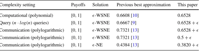
Table 1 Comparison of our approximation guarantees with the previous best-known guarantees
Complexity setting Payoffs Solution Previous best approximation This paper
Computational (polynomial) [0,1] -WSNE 0.6608 [10] 0.6528 Query (n·log(n)queries) [0,1] -WSNE 0.6667 [9] 0.6528+ Communication (polylogarithmic) [0,1] -WSNE 0.7321 [13] 0.6528+ Communication (polylogarithmic) {0,1} -WSNE 0.7321 [13] 0.5+ Communication (polylogarithmic) [0,1] -NE 0.4384 [13] 0.3820+
0.6528-WSNE. Moreover, the base algorithm can be implemented as a communi-cation efficient algorithm for finding a(12+)-WSNE in awin-losebimatrix game, where all payoffs are either 0 or 1.
The algorithm can also be used to beat the best known bound in the query complexity setting. It has already been shown by Goldberg and Roth [14] that an-NE of a zero-sum gamecan be found by a randomized algorithm that usesO(nlog2n)payoff queries. Since the rest of the steps used by our algorithm can also be carried out usingO(nlogn)
payoff queries, this gives us a query efficient algorithm for finding a 0.6528-WSNE. We also show that the base algorithm can be adapted to find a3−
√ 5
2 -NE in a bimatrix
game. Once again, this can be implemented in a communication efficient manner, and so we obtain an algorithm that computes a(3−
√ 5
2 +)-NE (i.e., 0.382-NE) using only
poly-logarithmic communication.
Finally, we provide a lower bound against the base algorithm that is essentially tight, namely within 0.0034 of the theoretical upper bound.
2 Preliminaries
Bimatrix GamesThroughout, we use[n]to denote the set{1,2, . . . ,n}. Ann×n
bimatrix game is a pair(R,C)of twon×nmatrices:Rgives payoffs for therowplayer andCgives the payoffs for thecolumnplayer. We make the standard assumption that all payoffs lie in the range[0,1]. For simplicity, as in [13], we assume that each payoff has constant bit-length.1Awin-losebimatrix game has all payoffs in{0,1}.
Each player hasn purestrategies. To play the game, both players simultaneously select a pure strategy: the row player selects a rowi ∈ [n], and the column player selects a column j ∈ [n]. The row player then receives payoffRi,j, and the column player receives payoffCi,j.
Amixed strategyis a probability distribution over[n]. We denote a mixed strategy for the row player as a vectorxof lengthn, such thatxi is the probability that the row player assigns to pure strategyi. A mixed strategy of the column player is a vectoryof lengthn, with the same interpretation. Given a mixed strategyxfor either player, the
supportofxis the set of pure strategiesiwithxi >0. Ifxandyare mixed strategies
for the row and the column player, respectively, then we call(x,y)amixed strategy profile. The expected payoff for the row player under strategy profile(x,y)is given byxTRyand for the column player byxTCy. We denote thesupportof a strategyx
as supp(x), which gives the set of pure strategiesi such thatxi >0.
Nash EquilibriaLetybe a mixed strategy for the column player. The set ofpure best responsesagainstyfor the row player is the set of pure strategies that maximize the payoff againsty. More formally, a pure strategyi∈ [n]is a best response againstyif, for all pure strategiesi∈ [n]we have:j∈[n]yj·Ri,j ≥
j∈[n]yj ·Ri,j. Column player best responses are defined analogously.
A mixed strategy profile(x,y)is amixed Nash equilibriumif every pure strategy in supp(x)is a best response againsty, and every pure strategy in supp(y)is a best response against x. Nash [18] showed that all bimatrix games have a mixed Nash equilibrium.
Approximate EquilibriaThere are two commonly studied notions of approximate equilibrium, and we consider both of them in this paper. The first notion is of an
-approximate Nash equilibrium(-NE), which weakens the requirement that a player’s expected payoff should be equal to their best response payoff. Formally, given a strat-egy profile(x,y), we define theregretsuffered by the row player to be the difference between the best response payoff and actual payoff, i.e.,
max i∈[n]
(R·y)i
−xT ·R·y.
The termR·yis a vector where theith entry of the vector,(R·y)i, corresponds the payoff the row player gets from playing hisith pure strategy when the column player playsy. Hence, the maximum over this vector is the best response payoff for the row player. The termxT · R·yencodes the expected payoff to the row player under the strategy profile(x,y).
Regret for the column player is defined analogously. We have that(x,y)is an-NE if and only if both players have regret less than or equal to.
The other notion is of an-approximate-well-supported equilibrium (-WSNE), which weakens the requirement that players only place probability on best response strategies. Given a strategy profile(x,y)and a pure strategy j ∈ [n], we say that jis an-best-response for the row player if
max i∈[n]
(R·y)i
−(R·y)j ≤.
An-WSNE requires that both players only place probability on-best-responses. In an-WSNE both players place probability only on-best-responses. Formally, the row player’spure strategy regretunder(x,y)is defined to be
max i∈[n]
(R·y)i
− min
i∈supp(x)
(R·y)i
.
Pure strategy regret for the column player is defined analogously. A strategy profile
Communication Complexity We consider the communication model for bimatrix games introduced by Goldberg and Pastink [13]. In this model, both players know the payoffs in their own payoff matrix, but do not know the payoffs in their opponent’s matrix. The players then follow an algorithm that uses a number of communication rounds, where in each round they exchange a single bit of information. Between each communication round, the players are permitted to perform arbitrary randomized computations (although it should be noted that, in this paper, the players will only perform polynomial-time computations) using their payoff matrix, and the bits that they have received so far. At the end of the algorithm, the row player outputs a mixed strategyx, and the column player outputs a mixed strategyy. The goal is to produce a strategy profile(x,y)that is an-NE or-WSNE for a sufficiently smallwhile limiting the number of communication rounds used by the algorithm. The algorithms given in this paper will use at most O(log2n)communication rounds. In order to achieve this, we use the following result of Goldberg and Pastink [13].
Lemma 1 ([13])Given a mixed strategyxfor the row-player and an >0, there is a randomized expected-polynomial-time algorithm that uses O(log22n)-communication
to transmit a strategyxs to the column player where|supp(xs)| ∈ O(log2n)and for
every strategy i ∈ [n]we have:
|(xT ·R)i−(xTs ·R)i| ≤.
The algorithm uses the well-known sampling technique of Lipton, Markakis, and Mehta to construct the strategyxs, so for this reason we will call the strategyxs the
sampled strategyfromx. Since this strategy has a logarithmically sized support, it can be transmitted by sendingO(log2n)strategy indexes, each of which can be represented using logn bits. By symmetry, the algorithm can obviously also be used to transmit approximations of column player strategies to the row player.
Query Complexity In the query complexity setting, the algorithm knows that the players will play ann×ngame(R,C), but it does not know any of the entries ofRor
C. These payoffs are obtained usingpayoff queriesin which the algorithm proposes a pure strategy profile(i,j), and then it is told the value of Ri j andCi j. After each payoff query, the algorithm can make arbitrary computations (although, again, in this paper the algorithms that we consider take polynomial time) in order to decide the next pure strategy profile to query. After making a sequence of payoff queries, the algorithm then outputs a mixed strategy profile(x,y). Again, the goal is to ensure that this strategy profile is an-NE or-WSNE, while minimizing the number of queries made overall.
There are two results that we will use for this setting. Goldberg and Roth [14] have given a randomized algorithm that, with high probability, finds an-NE of a zero-sum game usingO(n·log2n)payoff queries. Given a mixed strategy profile(x,y), an
players using O(n·log2 n)payoff queries and that succeeds with high probability. We summarise these two results in the following lemma.
Lemma 2 ([9,14])Given an n×n zero-sum bimatrix game, with probability at least
(1−n−18)(1−2 n)
2, we can compute an-Nash equilibrium(x,y), and-approximate
payoff vectors for both players under(x,y), using O(n·log2 n)payoff queries.
3 The Base Algorithm
In this section, we introduce thebase algorithm, which provides a simple way to find a
2
3-WSNE. We present this algorithm separately for three reasons. Firstly, the algorithm
is interesting in its own right, since it provides a relatively straightforward method for finding a23-WSNE that is quite different from the technique used in the KS-algorithm. Secondly, our algorithm for finding a 0.6528-WSNE will build on this algorithm and replace its final step with two more involved procedures. Thirdly, at the end of this section, we show how this algorithm can be adapted to provide a communication efficient way to find a(0.5+)-WSNE in win-lose games.
Algorithm1
1. Solve the zero-sum games(R,−R)and(−C,C).
– Let(x∗,y∗)be a NE of(R,−R), and let(xˆ,yˆ)be a NE of(−C,C). – Letvr be the value secured byx∗in(R,−R), and letvcbe the value secured byyˆin(−C,C). Without loss of generality assume thatvc≤
vr.
2. Ifvr ≤2/3, then return(xˆ,y∗).
3. If for all j ∈ [n]it holds thatCTj ·x∗≤2/3, then return(x∗,y∗). 4. Otherwise:
– Letj∗be a pure best response tox∗.
– Find a rowi such thatRij∗>1/3 andCij∗ >1/3. – Return(i,j∗).
We argue that this algorithm is correct. For that, we must prove that the rowiused in Step4actually exists.
Lemma 3 If Algorithm1reaches Step4, then there exists a row i such that Rij∗>1/3
and Cij∗>1/3.
Proof Letibe a row sampled fromx∗. We will show that there is a positive probability that rowisatisfies the desired properties.
Thus, applying Markov’s inequality we obtain:
Pr
T ≥ 2
3
≤ E[T] 2/3 <0.5.
Since Pr(Rij∗ ≤ 13)=Pr(T ≥ 23)we can therefore conclude that Pr(Rij∗≤ 13) <0.5. The exact same technique can be used to prove that Pr(Cij∗≤ 13) <0.5, by using the fact thatCjT∗·x∗> 23.
We can now apply the union bound to argue that:
Pr
Rij∗≤
1
3 orCij∗≤ 1 3
<1.
Hence, there is positive probability that rowisatisfiesRij∗>31andCij∗ >13, so such a row must exist.
We now argue that the algorithm always produces a23-WSNE. There are three possible strategy profiles that can be returned by the algorithm, which we consider individually.
The algorithm returns in Step2Sincevc≤vrby assumption, and sincevr ≤ 23, we have that(R·y∗)i ≤ 23for every rowi, and((xˆ)T·C)j ≤ 23for every column j. So, both players can have pure strategy regret at most 23 in(xˆ,y∗), and thus this profile is a23-WSNE.
The algorithm returns in Step3Much like in the previous case, when the column player playsy∗, the row player can have pure strategy regret at most23; observe that in this case the row player actually suffers zero regret sincex∗is a best response againsty∗. The requirement thatCTjx∗ ≤ 23 also ensures that the column player has pure strategy regret at most23. Thus, we have that(x∗,y∗)is a 23-WSNE.
The algorithm returns in Step4Both players have payoff at least 13under(i,j∗)
for the sole strategy in their respective supports. Hence, the maximum pure strategy regret that can be suffered by a player is 1−13 =23.
Observe that the zero-sum games solved in Step1can be solved via linear program-ming, and so the algorithm runs in polynomial time. Therefore, we have shown the following.
Theorem 4 Algorithm1always produces a23-WSNE in polynomial time.
3.1 Win-Lose Games
Formally, we will study the following simple modification of Algorithm 1.
Algorithm2
1. Solve the zero-sum games(R,−R)and(−C,C).
– Let(x∗,y∗)be a NE of(R,−R), and let(xˆ,yˆ)be a NE of(C,−C). – Letvr be the value secured byx∗in(R,−R), and letvcbe the value
secured byyˆin(−C,C). Without loss of generality assume thatvc≤
vr.
2. Ifvr ≤0.5, then return(xˆ,y∗).
3. If for all j ∈ [n]it holds thatCTj ·x∗≤0.5, then return(x∗,y∗). 4. Otherwise:
– Letj∗be a pure best response tox∗.
– Find a rowi such thatRij∗=1 andCi j =1. – Return(i,j∗).
We will show that this algorithm always finds a 0.5-WSNE in a win-lose game. Firstly, we show that the pure Nash equilibrium found in Step4always exists. The following lemma is similar to Lemma3, but exploits the fact that the game is win-lose to obtain a stronger conclusion.
Lemma 5 If Algorithm2is applied to a win-lose game, and it reaches Step4, then there exists a row i ∈supp(x∗)such that Rij∗ =1and Cij∗=1.
Proof Letibe a row sampled fromx∗. We will show that there is a positive probability that rowisatisfies the desired properties.
We begin by showing that the probability that Pr(Rij∗=0) <0.5. Let the random variableT = 1−Rij∗. Sincevr > 12, we have that E[T] < 0.5. Thus, applying Markov’s inequality we obtain:
Pr(T ≥1)≤ E[T] 1 <0.5.
Since Pr(Rij∗=0)=Pr(T ≥1)we can therefore conclude that Pr(Rij∗=0) <0.5. The exact same technique can be used to prove that Pr(Cij∗=0) <0.5, by using the fact thatCjT∗·x∗>0.5.
We can now apply the union bound to argue that:
Pr(Rij∗=0 orCij∗=0) <1.
Hence, there is positive probability that rowisatisfiesRij∗>0 andCij∗ >0, so such a row must exist. The final step is to observe that, since the game is win-lose, we have thatRij∗>0 impliesRij∗=1, and thatCij∗>0 impliesCij∗=1.
Communication ComplexityWe now show that Algorithm 2 can be implemented in a communication efficient way.
The zero-sum games in Step 1 can be solved by the two players independently without any communication. Then, the players exchange vr andvs using O(logn) rounds of communication. If bothvr andvsare smaller than 0.5, then the players use the algorithm from Lemma1to communicatexˆs andy∗s between themselves, using the parameter2in place of. Since the payoffs under the sampled strategies are within
2 of the originals, we have that all pure strategies have payoff less than or equal to
0.5+under(xˆs,y∗s), so this strategy profile is a(0.5+)-WSNE.
We will assume from now on thatvr > vc. If the algorithm reaches Step3, then the row player uses the algorithm of Lemma1to communicatex∗s to the column player. The column player then computes a best responsej∗s againstx∗s, and checks whether the payoff ofj∗s againstx∗s is less than or equal to 0.5+. If so, then the players output
(x∗s,j∗s), which is a(0.5+)-WSNE
Otherwise, we claim that there is a pure strategyi ∈ supp(x∗s)such that(i,j∗s)is a pure Nash equilibrium. This can be shown by observing that the expected payoff of x∗s againstj∗s is at least 0.5−, while the expected payoff ofj∗s againstx∗s is at least 0.5+. Repeating the proof of Lemma5using these inequalities then shows that the pure Nash equilibrium does indeed exist. Since supp(x∗s)has logarithmic size, the row player can simply transmit to the column player all payoffs Rij∗s for which
i ∈supp(x∗s), and the column player can then send back a row corresponding to a pure Nash equilibrium.
In conclusion, we have shown the following theorem.
Theorem 6 For every win-lose game and > 0, there is a randomized expected-polynomial-time algorithm that finds a(0.5+)-WSNE with O
log2n
2
communica-tion.
4 An Algorithm for Finding a 0
.
6528-WSNE
In this section, we show how Algorithm 1 can be modified to produce a 0.6528-WSNE.
OutlineOur algorithm replaces Step4of Algorithm 1 with a more involved procedure. This procedure uses two techniques, that both find an-WSNE with < 23. Firstly, we attempt to turn(x∗,j∗)into a WSNE byshifting probabilities. Observe that, sincej∗ is a best response, the column player has a pure strategy regret of 0 in(x∗,j∗). On the other hand, we have no guarantees about the row player sincex∗might place a small amount of probability strategies with payoff strictly less than 13. However, sincex∗
If shifting probabilities fails to find an-WSNE with < 23, then we show that the game contains amatching penniessub-game. More precisely, we show that there exists a columnj, and rowsbandssuch that the 2×2 sub-game induced byj∗,j,b, andshas the following form:
@ @
I II
b
s
j∗ j
≈1 0
0 ≈1
0 ≈1
≈1 0
Thus, if both players play uniformly over their respective pair of strategies, thenj∗,j,
b, andswith have payoff≈0.5, and so this yields an-WSNE with < 23.
The AlgorithmWe now formalize this approach, and show that it always finds an
-WSNE with < 23. In order to quantify the precisethat we obtain, we parametrise the algorithm by a variablez, which we constrain to be in the range 0≤z< 241. With the exception of the matching pennies step, all other steps of the algorithm will return a(23−z)-WSNE, while the matching pennies step will return a(12+ f(z))-WSNE for some increasing function f. Optimizing the trade off between 23−zand21+ f(z)
then allows us to determine the quality of WSNE found by our algorithm.
The algorithm is displayed as Algorithm 3. Steps1,2, and3are versions of the corresponding steps from Algorithm 1, which have been adapted to produce a(23−z) -WSNE. Step4implements the probability shifting procedure, while Step5finds a matching pennies sub-game.
Observe that the probabilities used in xmp andymp are only well defined when
z ≤ 241, because we have that 21−−1539zz > 1 whenever z > 241, which explains our required upper bound onz.
The correctness of Step5This step of the algorithm relies on the existence of the rowsbands, which is shown in the following lemma.
Lemma 7 Suppose that the following conditions hold:
1. x∗has payoff at least23−z againstj∗. 2. j∗has payoff at least 23−z againstx∗. 3. x∗has payoff at least23−z againstj.
4. Neitherj∗norjcontains a pure(23−z)-WSNE(i,j)with i ∈supp(x∗).
Then, both of the following are true:
– There exists a row b∈B such that Rbj∗>1−118+3zz and Cbj >1−118+3zz.
– There exists a row s∈S such that Csj∗ >1−127+3zz and Rsj >1−127+3zz.
Algorithm3
1. Solve the zero-sum games(R,−R)and(−C,C).
– Let(x∗,y∗)be a NE of(R,−R), and let(xˆ,yˆ)be a NE of(C,−C).
– Letvrbe the value secured byx∗in(R,−R), and letvcbe the value secured byyˆin (−C,C). Without loss of generality assume thatvc≤vr.
2. Ifvr ≤2/3−z, then return(xˆ,y∗).
3. If for allj∈ [n]it holds thatCTjx∗≤2/3−z, then return(x∗,y∗).
4. Otherwise:
– Letj∗be a pure best response againstx∗. Define:
S:= {i∈supp(x∗):Rij∗<1/3+z} B:=supp(x∗)\S
– Define the strategyxBas follows. For eachi∈ [n]we have:
(xB)i= 1
Pr(B)·x∗i ifi∈B 0 otherwise.
– If(xBT·C)j∗≥1
3+z, then return(xB,j∗).
5. Otherwise:
– Letjbe a pure best response againstxB.
– If there exists ani∈supp(x∗)such that(i,j∗)or(i,j)is a pure(23−z)-WSNE, then return it.
– Find a rowb∈Bsuch thatRbj∗>1−1+318zzandCbj>1−1+318zz. – Find a rows∈Ssuch thatCsj∗>1−127+3zzandRsj>1−127+3zz.
– Define the row player strategyxmpand the column player strategyympas follows. For
eachi∈ [n]we have:
xmpi=
⎧ ⎪ ⎨ ⎪ ⎩
1−24z
2−39z ifi=b, 1−15z
2−39z ifi=s, 0 otherwise.
ympi=
⎧ ⎪ ⎨ ⎪ ⎩
1−24z
2−39z ifi=j∗, 1−15z
2−39z ifi=j, 0 otherwise.
– Return(xmp,ymp).
because, due to Step2, we know thatx∗is a min-max strategy that secures payoff at leastvr >23−z. The second condition holds because Step3ensures that the column player’s best response payoff is at least 23 −z. The fourth condition holds because Step5explicitly checks for these pure strategy profiles.
Quality of Approximation We now analyse the quality of WSNE our algorithm produces. Steps2,3,4, and 5 each return a strategy profile. Observe that Steps2 and3are the same as the respective steps in the base algorithm, but with the threshold changed from 23 to23−z. Hence, we can use the same reasoning as we gave for the base algorithm to argue that these steps return(23−z)-WSNE. We now consider the other two steps.
The algorithm returns in Step4By definition all rowsr ∈ BsatisfyRij∗ ≥ 13+z,
1−(13+z)= 23−z. For the same reason, since(xBT ·C)j∗≥ 13+zholds, the pure strategy regret of the column player can also be at23 −z. Thus, the profile
(xB,j∗)is a(23−z)-WSNE.
The algorithm returns in Step5SinceRbj∗ >1−118+3zz, the payoff ofbwhen the column player playsympis at least:
1−24z
2−39z·
1− 18z 1+3z
=1−39z+360z2 2−33z−117z2
Similarly, sinceRsj >1−127+3zz, the payoff ofswhen the column player plays
ympis at least:
1−15z
2−39z·
1− 27z 1+3z
=1−39z+360z2 2−33z−117z2
In the same way, one can show that the payoffs ofj∗andjare also12−−3933zz+−117360zz22 when
the row player playsxmp. Thus, we have that(xmp,ymp)is a(1−12−−3933zz+−360117zz22) -WSNE.
To find the optimal value forz, we need to find the largest value ofzfor which the following inequality holds.
1−1−39z+360z
2
2−33z−117z2 ≤
2 3 −z.
Setting the inequality to an equality and rearranging gives us a cubic polynomial equation: 117z3+432z2−30z+13=0.Since the discriminant of this polynomial is positive, this polynomial has three real roots, which can be found via the trigonometric method. Only one of these roots lies in the range 0≤z< 241, which is the following:
z= 1
117 √
3
√
2434√3 cos
1 3 arctan
39 240073
√ 9749√3
−3√2434 sin
1 3 arctan
39 240073
√ 9749√3
−48√3
.
Thus, we getz≈0.013906376, and we have found an algorithm that always produces a 0.6528-WSNE. So we have the following theorem.
4.1 Proof of Lemma7
In this section we assume that Steps1 through4 of our algorithm did not return a
(2
3−z)-WSNE, and that neitherj∗norjcontained a pure( 2
3−z)-WSNE. We show
that, under these assumptions, the rowsbandsrequired by Step5do indeed exist.
Probability BoundsWe begin by proving bounds on the amount of probability thatx∗
can place onSandB. The following lemma uses the fact thatx∗secures an expected payoff of at least 23−zto give an upper bound on the amount of probability thatx∗
can place onS. To simplify notation, we use Pr(B)to denote the probability assigned byx∗to the rows inB, and we use Pr(S)to denote the probability assigned byx∗to the rows inS.
Lemma 9 Pr(S)≤ 12+−33zz.
Proof We will prove our claim using Markov’s inequality. Consider the random vari-ableT =1−Rij∗whereiis sampled fromx∗. Since by our assumption the expected payoff of the row player is greater than 2/3−zwe get thatE(T)≤ 1/3+z. If we apply Markov’s inequality we get
Pr
T ≥ 2
3 −z
≤ E2(T)
3−z
≤ 1+3z 2−3z
which is the claimed result.
Next we show an upper bound on Pr(B). Here we use the fact thatj∗ does not contain a(23−z)-WSNE to argue that all column player payoffs inBare smaller than
1
3+z. Since we know that the payoff ofj∗againstx∗is at least 2
3−z, this can be used
to prove a upper bound on the amount of probability thatx∗assigns toB.
Lemma 10 Pr(B)≤ 12+−33zz.
Proof Since there is noi ∈supp(x∗)such that(i,j∗)is a pure(23−z)-WSNE, and since each rowi∈ BsatisfiesRij∗≥ 13+z, we must have thatCij∗< 13+zfor every
i ∈ B. By assumption we know that CjT∗x∗ > 2/3−z. So, we have the following
inequality:
2
3 −z<Pr(B)·
1 3 +z
+1−Pr(B)·1.
Solving this inequality for Pr(B)gives the desired result.
Payoff Inequalities forj∗We now show properties about the average payoff obtained from the rows inBandS. Recall thatxBwas defined in Step4of our algorithm, and that it denotes the normalization of the probability mass assigned byx∗to rows inB. The following lemma shows that the expected payoff to the row player in the strategy profile(xB,j∗)is close to 1.
Proof By definition we have that:
(xBT ·R)j∗= 1
Pr(B)·
i∈B
x∗i ·Rij∗. (1)
We begin by deriving a lower bound fori∈Bx∗i ·Rij∗. Using the fact thatx∗secures an expected payoff of at least 2/3−zagainstj∗and then applying the bound from Lemma9gives:
2 3−z<
i∈B
x∗i ·Rij∗+
1 3+z
·Pr(S)
≤
i∈B
x∗i ·Rij∗+
1 3 +z
·1+3z 2−3z.
Hence we can conclude that:
i∈B
xi∗·Rij∗> 2 3 −z−
1 3 ·
(1+3z)2
2−3z
= 1−6z 2−3z.
Substituting this into Eq. (1), along with the upper bound on Pr(B)from Lemma10, allows us to conclude that:
(xBT ·R)j∗≥ 2−3z
1+3z ·
i∈B
xi∗·Rij∗
> 2−3z
1+3z·
1−6z
2−3z
= 1−6z 1+3z.
Next we would like to show a similar bound on the expected payoff to the column player of the rows inS. To do this, we definexSto be the normalisation of the probability mass thatx∗assigns to the rows inS. More formally, for eachi∈ [n], we define:
(xS)i =
1
Pr(S)·x∗i ifi∈ S
0 otherwise.
The next lemma shows that the expected payoff to the column player in the profile
(xS,j∗)is close to 1.
Proof By definition we have that:
(xST ·C)j∗= 1
Pr(S)·
i∈S
x∗i ·Cij∗. (2)
We begin by deriving a lower bound fori∈Sx∗i ·Cij∗. By assumption, we know that
CjT∗x∗>2/3−z. Moreover, sincej∗does not contain a(23−z)-WSNE we have that
all rowsiinBsatisfyCij∗≤1/3+z. If we combine these facts that with Lemma10 we obtain:
2 3−z<
i∈S
x∗i ·Cij∗+
1 3+z
·Pr(B)
≤
i∈S
x∗i ·Cij∗+
1 3 +z
·1+3z 2−3z.
Hence we can conclude that:
i∈S
x∗i ·Cij∗> 2 3−z−
1 3 ·
(1+3z)2
2−3z
= 1−6z 2−3z.
Substituting this into Eq. (2), along with the upper bound on Pr(S)from Lemma10, allows us to conclude that:
(xBT ·R)j∗≥ 2−3z
1+3z ·
i∈B
xi∗·Rij∗
> 2−3z
1+3z·
1−6z
2−3z
= 1−6z 1+3z.
Payoff Inequalities forjWe now want to prove similar inequalities for the column
j. The next lemma shows that the expected payoff for the column player in the profile
(xB,j)is close to 1. This is achieved by first showing a lower bound on the payoff to the column player in the profile(xB,j∗), and then using the fact thatj∗ is not a
(2
3−z)-best-response againstxB, and thatjis a best response againstxB.
Lemma 13 We have(xBT ·C)
j >11−+63zz.
Proof We first establish a lower bound on(xBT ·C)j∗. By assumption, we know that
CjT∗x∗>2/3−z. Using this fact, along with the bounds from Lemmas9and10gives:
2
≤ 1+3z 2−3z ·(xB
T ·
C)j∗+1+3z
2−3z.
Solving this inequality for(xBT ·C)j∗yields:
(xBT ·C)j∗> 1
3 ·
1−21z+9z2
1+3z .
Now we can prove the lower bound on(xBT ·C)j. Sincej∗is not a(23−z) -best-response againstxB, and sincejis a best response againstxBwe obtain:
(xBT ·C)j > (xBT ·C)j∗+2
3 −z
(xBT ·C)j > 1
3·
1−21z+9z2
1+3z +
2 3 −z
= 1−6z 1+3z.
The only remaining inequality that we require is a lower bound on the expected payoff to the row player in the profile(xS,j). However, before we can do this, we must first prove an upper bound on the expected payoff to the row player in(xB,j), which we do in the following lemma. Here we first prove that most of the probability mass ofxBis placed on rowsiin whichCij > 13+z, which when combined with the fact that there is noi∈supp(x∗)such that(i,j)is a pure(23−z)-WSNE, is sufficient to provide an upper bound.
Lemma 14 We have(xBT ·R)j <13·1+331+z3+z9z2.
Proof We begin by proving an upper bound on the amount of probability mass assigned byxBto rowsi withCij < 13+z. LetT =1−Cij be a random variable where the rowiis sampled according toxB. Lemma13implies that:
E[T]<1−1−6z 1+3z =
9z
1+3z.
Observe that Pr(T ≥ 1−(13 +z)) = Pr(T ≥ 23 −z)is equal to the amount of probability thatxBassigns to rowsiwithCij <13+z. Applying Markov’s inequality then establishes our bound.
Pr
T ≥ 2
3 −z
≤
9z
1+3z
2 3−z
.
i ∈supp(x∗)such that(i,j)is a pure(23−z)-WSNE, we know that any such rowi
must satisfyRij < 13+z. Hence, we obtain the following bound:
(xBT ·R)j < (1−p)·
1 3 +z
+p
= 1
3 ·
1+33z+9z2
1+3z .
Finally, we show that the expected payoff to the row player in the profile(xS,j)is close to 1. Here we use the fact thatx∗is a min-max strategy along with the bound from Lemma14to prove our lower bound.
Lemma 15 We have(xST ·R)j > 11−+153zz.
Proof Sincex∗is a min-max strategy that secures a value strictly larger than 23−z, we have:
2
3−z<Pr(B)·(xB T ·
R)j+Pr(S)·(xST ·R)j.
Substituting the bounds from Lemmas9,10, and14then gives:
2 3−z<
1+3z
2−3z·
1 3 ·
1+33z+9z2
1+3z +
1+3z
2−3z ·(xS
T ·R) j.
Solving for(xST ·R)j then yields the desired result.
Finding rowsband u So far, we have shown that the expected payoff to the row player in(xB,j∗)is close to 1, and that the expected payoff to the column player in
(xB,j)is close to 1. We now show that there exists a rowb∈ Bsuch thatRbj∗is close to 1, andCbj is close to 1, and that there exists a rows ∈ S in whichCsj∗ andRsj are both close to 1. The following lemma uses Markov’s inequality to show a pair of probability bounds that will be critical in showing the existence ofb.
Lemma 16 We have:
– xBassigns strictly more than0.5probability to rows i with Rij∗>1−118+3zz.
– xBassigns strictly more than0.5probability to rows i with Cij >1−118+3zz.
Proof We begin with the first case. Consider the random variableT =1−Rij∗where
iis sampled fromxB. By Lemma11, we have that:
E[T]<1−1−6z 1+3z =
9z
1+3z.
We have that T ≥ 118+3zz whenever Rij∗ ≤ 1 − 118+3zz, so we can apply Markov’s inequality to obtain:
Pr
T ≥ 18z
1+3z
<
9z
1+3z
The proof of the second case is identical to the proof given above, but uses the (identical) bound from Lemma13.
The next lemma uses the same techniques to prove a pair of probability bounds that will be used to prove the existence ofs.
Lemma 17 We have:
– xSassigns strictly more than 13probability to rows i with Cij∗ >1−127+3zz.
– xSassigns strictly more than 23probability to rows i with Rij >1−127+3zz.
Proof We begin with the first claim. Consider the random variableT = 1−Cij∗ wherei is sampled fromxS. By Lemma12, we have that:
E[T]<1−1−6z 1+3z =
9z
1+3z.
We have that T ≥ 127+3zz whenever Cij∗ ≤ 1− 127+3zz, so we can apply Markov’s inequality to obtain:
Pr
T ≥ 27z
1+3z
<
9z
1+3z
27z
1+3z
= 1
3.
We now move on to the second claim. Consider the random variableT =1−Rij∗ wherei is sampled fromxB. By Lemma15, we have that:
E[T]<1−1−15z 1+3z =
18z
1+3z.
We have that T ≥ 127+3zz whenever Rij∗ ≤ 1 − 127+3zz, so we can apply Markov’s inequality to obtain:
Pr
T ≥ 27z
1+3z
<
18z
1+3z
27z
1+3z
= 2
3.
Finally, we can formally prove the existence ofbands, which completes the proof of correctness for our algorithm.
Proof of Lemma7 We begin by proving the first claim. If we sample a rowbrandomly fromxB, then Lemma16implies that probability thatRbj∗≤1−118+3zz is strictly less than 0.5 and that the probability thatCbj ≤1−118+3zz is strictly less than 0.5. Hence, by the union bound, the probability that at least one of these events occurs is strictly less than 1. So, there is a positive probability that neither of the events occurs, which implies that there exists at least one rowbthat satisfies the desired properties.
5 Communication Complexity
We claim that Algorithm 3 can be adapted for the limited communication setting. We make the following modification to our algorithm. After computingx∗,y∗,xˆ,andyˆ, we then use Lemma1to construct and communicate the sampled strategiesx∗s,ys∗,xˆs,and ˆ
ys. These strategies are communicated between the two players using 4·(logn)2bits of communication, and the players also exchangevr =(x∗s)T ·Ry∗s andvc= ˆxsTCyˆs using lognrounds of communication. The algorithm then continues as before, except the sampled strategies are used in place of their non-sampled counterparts. Finally, in Steps2and3, we test against the threshold23−z+instead of23−z.
Observe that, when sampled strategies are used, all steps of the algorithm can be carried out in at most(logn)2communication. In particular, to implement Step4, the column player can communicatej∗ to the row player, and then the row player can communicate Rij∗ for all rowsi ∈ supp(x∗s)using(logn)2 bits of communication, which allows the column player to determinej. Oncej has been determined, there are only 2·lognpayoffs in each matrix that are relevant to the algorithm (the payoffs in rowsi ∈supp(x∗s)in columnsj∗andj,) and so the two players can communicate all of these payoffs to each other, and then no further communication is necessary.
Now, we must argue that this modified algorithm is correct. Firstly, we argue that if the modified algorithm reaches Step5, then the rowsbandsexist. To do this, we observe that the required preconditions of Lemma7 are satisfied byx∗s,j∗, andj. Condition 2 holds because the modified Step3ensures that the column player’s best response payoff is at least 23−z+ > 23−z, while Condition 4 is ensured by the explicit check in Step5. For Conditions 1 and 3, we use the fact that(x∗,y∗)is an
-Nash equilibrium of the zero-sum game(R,−R). The following lemma shows that any approximate Nash equilibrium of a zero-sum game behaves like an approximate min-max strategy.
Lemma 18 If(x,y)is an-NE of a zero-sum game(M,−M), then for every strategy ywe have:
xT ·M·y≥xT ·M·y−.
Proof Letv =xT ·M ·ybe the payoff to the row player under(x,y). Suppose, for the sake of contradiction, that there exists a column player strategyysuch that:
xT ·M·y< v−.
Since the game is zero-sum, this implies that the column player’s payoff under(x,y)
is strictly larger than−v+, which then directly implies that the best response payoff for the column player against x is strictly larger than−v+. However, since the column player’s expected payoff under(x,y)is−v, this then implies that(x,y)is not an-NE, which provides our contradiction.
Finally, we argue that the algorithm finds a(0.6528+). The modified Steps 2 and3now return a(23−z+)-WSNE, whereas the approximation guarantees of the other steps are unchanged. Thus, we our original analysis gives the following theorem.
Theorem 19 For every >0, there is a randomized expected-polynomial-time algo-rithm that uses O
log2n
2
communication and finds a(0.6528+)-WSNE.
6 Query Complexity
We now show that Algorithm 3 can be implemented in a payoff-query efficient manner. Let >0 be a positive constant. We now outline the changes needed in the algorithm.
– In Step1we use the algorithm of Lemma2to find2-NEs of(R,−R), and(C,−C). We denote the mixed strategies found as(x∗a,y∗a)and(xˆa,yˆa), respectively, and we use these strategies in place of their original counterparts throughout the rest of the algorithm. We also compute2-approximate payoff vectors for each of these strategies, and use them whenever we need to know the payoff of a particular strategy under one of these strategies. In particular, we setvr to be the payoff ofx∗a according to the approximate payoff vector ofy∗a, and we setvcto be the payoff ofyˆaaccording to the approximate payoff vector forxˆa.
– In Steps2and3we test against the threshold of 23−z+rather than23−z. – In Step4we select j∗to be the column that is maximal in the approximate payoff
vector againstx∗a. We then spendn payoff queries to query every row in column
j∗, which allow us to proceed with the rest of this step as before.
– In Step5we use the algorithm of Lemma2to find an approximate payoff vectorv for the column player againstxB. We then selectjto be a column that maximizes
v, and then spendn payoff queries to query every row inj∗, which allows us to proceed with the rest of this step as before.
Observe that the query complexity of the algorithm isO(n·log2n), where the dom-inating term arises due to the use of the algorithm from Lemma 2to approximate solutions to the zero-sum games.
We now argue that this modified algorithm produces a(0.6528+)-WSNE. Firstly, we need to reestablish the existence of the rowsbandsused in Step5. To do this, we observe that the preconditions of Lemma7hold forx∗a. We start with Conditions 1 and 3. Note that the payoff for the row player under(x∗a,y∗a)is at leastvr−2(sincevr was estimated with approximate payoff vectors,) and Step2ensures thatvr > 23−z+. Hence, we can apply Lemma18to argue thatx∗asecures payoff at least23−zagainst
every strategy of the column player, which proves that Conditions 1 and 3 hold. Condition 2 holds because the check in Step3, ensures that the approximate payoff of
j∗againstx∗is at least23−z+, and therefore the actual payoff of of j∗againstx∗
is at least23−z+2. Finally, Condition 4 holds because pure strategy profiles of this form are explicitly checked for in Step5.
Theorem 20 There is a randomized algorithm that, with high probability, finds a
(0.6528+)-WSNE using O(n·log2n)payoff queries.
7 A communication-efficient algorithm for finding a
(
0
.
382
+
)
-NE
We study the following algorithm.
Algorithm4
1. Solve the zero-sum games(R,−R)and(−C,C).
– Let(x∗,y∗)be a NE of(R,−R), and let(xˆ,yˆ)be a NE of(C,−C). – Letvr be the value secured byx∗in(R,−R), and letvcbe the value
secured byyˆin(−C,C). Without loss of generality assume thatvc≤
vr. – Ifvr ≤ 3−
√ 5
2 , return(xˆ,y∗).
2. Otherwise:
– Letj be a best response for the column player againstx∗. – Letrbe a best response for the row player against j. – Define the strategy profilex= 2−1v
r ·x
∗+1−vr 2−vr ·r.
– Return(x,j).
We show that this algorithm always produces a 3−
√ 5
2 -NE. We start by considering
the strategy profile returned by Step1. The maximum payoff that the row player can achieve againsty∗isvr, so the row player’s regret can be at mostvr. Similarly, the maximum payoff that the column layer can achieve againstxˆisvc≤vr, so the column player’s regret can be at mostvr. Step1only returns a strategy profile in the case where
vr ≤ 3−
√ 5
2 , so this step always produces a 3−√5
2 -NE.
To analyse the quality of approximate equilibrium found by Step2, we use the following Lemma.
Lemma 21 The strategy profile(x,j)is a 1−vr 2−vr-NE.
Proof We start by analysing the regret of the row player. By definition, rowris a best response against column j. So, the regret of the row player can be expressed as:
Rr j −(x·R)j =Rr j − 1 2−vr ·((
x∗)T ·R)j− 1−vr 2−vr ·
Rr j
≤ 1
2−vr ·
Rr j − 1 2−vr ·vr
≤ 1
2−vr ·
1− 1
2−vr ·vr
= 1−vr 2−vr
,