Compact and low complexity binary feature descriptor and Fisher Vectors for video analytics

warwick.ac.uk/lib-publications

Manuscript version: Author’s Accepted Manuscript

The version presented in WRAP is the author’s accepted manuscript and may differ from the

published version or Version of Record.

Persistent WRAP URL:

http://wrap.warwick.ac.uk/126736

How to cite:

Please refer to published version for the most recent bibliographic citation information.

If a published version is known of, the repository item page linked to above, will contain

details on accessing it.

Copyright and reuse:

The Warwick Research Archive Portal (WRAP) makes this work by researchers of the

University of Warwick available open access under the following conditions.

Copyright © and all moral rights to the version of the paper presented here belong to the

individual author(s) and/or other copyright owners. To the extent reasonable and

practicable the material made available in WRAP has been checked for eligibility before

being made available.

Copies of full items can be used for personal research or study, educational, or not-for-profit

purposes without prior permission or charge. Provided that the authors, title and full

bibliographic details are credited, a hyperlink and/or URL is given for the original metadata

page and the content is not changed in any way.

Publisher’s statement:

Please refer to the repository item page, publisher’s statement section, for further

information.

Compact and Low-complexity Binary Feature

Descriptor and Fisher Vectors for Video Analytics

Roberto Leyva, Victor Sanchez,

Member IEEE, and Chang-Tsun Li,

Senior Member IEEE

Abstract—In this paper, we propose a compact and low-complexity binary feature descriptor for video analytics. Our binary descriptor encodes the motion information of a spatio-temporal support region into a low-dimensional binary string. The descriptor is based on a binning strategy and a construction that binarizes separately the horizontal and vertical motion components of the spatio-temporal support region. We pair our descriptor with a novel Fisher Vector (FV) scheme for binary data to project a set of binary features into a fixed length vector in order to evaluate the similarity between feature sets. We test the effectiveness of our binary feature descriptor with FVs for action recognition, which is one of the most challenging tasks in computer vision, as well as gait recognition and animal behavior clustering. Several experiments on the KTH, UCF50, UCF101, CASIA-B, and TIGdog datasets show that the proposed binary feature descriptor outperforms the state-of-the-art feature descriptors in terms of computational time and memory and stor-age requirements. When paired with FVs, the proposed feature descriptor attains a very competitive performance, outperforming several state-of-the-art feature descriptors and some methods based on convolutional neural networks.

Index Terms—binary features, video analysis, Fisher Vectors, CNN.

I. INTRODUCTION

Nearly a million minutes of video content circulate on the internet every second [1]. Due to this dramatic growth, it is necessary to explore and design efficient methods to analyze video data [2], e.g., for summarization [3], classification [4, 5], action recognition [6, 7], video surveillance [8, 9], and abnormal event detection [10, 11]. Convolutional Neural Networks (CNNs) and approaches based on hand-crafted fea-ture descriptors have demonstrated outstanding performance for several video analysis tasks. However, in many cases, these approaches may require a vast amount of computational resources to extract and process the extracted features. This is a major concern for CNNs, which may require up to months to complete the training process even if clusters or powerful servers are used [12]. Although methods based on hand-crafted feature descriptors tend to require shorter training and process-ing times than those based on deep neural networks, the high-dimensionality of some of the extracted feature descriptors demands vast storage capacities and computational resources,

Roberto Leyva, Victor Sanchez, and Chang-Tsun Li are with the Computer Science Department at University of Warwick, Coventry, United Kingdom.

Roberto Leyva is also with the University of Essex. Chang-Tsun Li is also with the School of Information Technology, Deakin University, Geelong, Australia.

This work was funded by the Mexican Ministry of Education - CONACyT and the EU Horizon 2020 project, entitled Computer Vision Enabled Multi-media Forensics and People Identification (acronym: IDENTITY, Project ID: 690907)

thus hindering their implementation on low-cost devices and conventional machines [7, 13]. Developing low-complexity, compact and efficient feature descriptors for video analytics is therefore an important challenge.

Inspired by other efficient and low-complexity binary fea-ture descriptors for images [14–21], this work further improves our binary feature descriptor for video in [22, 23] by increas-ing its descriptiveness power and reducincreas-ing its computational complexity. Furthermore, we propose to pair our descriptor with Fisher Vectors (FVs) for binary data, which is a high-order mapping technique that projects a set of binary features into a fixed-length vector to effectively evaluate the similarity among feature sets. The main contributions of this work are as follows:

• Our binary feature descriptor captures motion information from two sources, i.e., optical flow and temporal gradi-ents. The latter is encoded independently for two motion components, which increases the descriptiveness power.

• We introduce a novel technique based on Integral Video (IV) to considerably reduce the computational complexity of our binary feature descriptor.

• We propose a novel FV formulation based on the

Per-ronin’s [24] assumptions of the Fisher kernel built on Bernoulli distributions, which allows simplifying the In-formation Matrix. To the best of our knowledge, this work is the first to formulate FVs using such assumptions on binary data.

• We paired our binary feature descriptor with FVs to project a set of binary features into a fixed-length vector. To the best of our knowledge, this work is the first to apply FVs to binary feature vectors extracted from video data.

To evaluate the compactness, computational complexity and descriptiveness power of our binary feature descriptor, we focus on action recognition, which is one of the most chal-lenging tasks in computer vision, as well as gait recognition and animal behavior clustering. Evaluations on the KTH, UFC101, UCF50, CASIA-B and TIGdog datasets show that our feature descriptor, when paired with our FVs, attains a very competitive performance with short processing times and low storage requirements, outperforming several binary and non-binary feature descriptors, as well as some methods based on CNNs.

to reduce the computational complexity and dimensionality of feature descriptors. In Section V, we explain in detail our improved binary feature descriptor and FV formulation. This section also includes a discussion of the complexity of our binary feature descriptor compared to that of CNNs. Experimental results and discussions are presented in Section V. We conclude this paper in Section VI.

II. PREVIOUSWORK

Local features: Features extracted from Spatio-Temporal Support Regions (STSR), i.e., local features [25–34], have been shown to attain a remarkable performance in various tasks including classification/recognition [6, 35, 36], summa-rization [3], and anomaly detection [11]. These local features are usually extracted from various motion information sources, such as intensity [25, 26], frequency transformations [27–29], 3D gradients [30–32], voxel texture [36] and optical flow [33, 34]. The descriptive power of their associated feature vectors [26, 37] is further improved by tracking and coding information from inhomogeneous patches [33, 34, 38–41], which is especially useful in complex backgrounds [42]. Unfortunately, besides their high-dimensionality [31–33], rep-resenting numerically these local features requires double-precision numbers [30–33, 33, 34]. Consequently, any further processing of the feature vectors, e.g., clustering and matching, inevitably involves very long computational times [19, 21, 31] and large memory and storage requirements [33, 34]. Impor-tant efforts have been made to tackle the high-dimensionality and high-complexity of local features [14, 43–47]. These efforts mainly include double-precision to binary projections [44–46, 48], which may be applied not only to local features [49], but also to those features extracted globally as high-order representations [43, 47]. Binary feature descriptors for video that do not rely on double-precision representations, e.g., [44, 45], have been rarely explored because of their relatively low-performance [50]. For the case of images, however, binary feature descriptors have been shown to attain a very good performance [17–21]. This motivates us to design a low-complexity and compact binary feature descriptor for video.

Fisher Vectors for binary data: Local features combined with FVs [34, 51, 52] have attracted much attention because of their superior performance compared to Bag of Features (BoF) representations [53]. FVs provide a more general way to define a kernel from a generative process of the data, as compared to BoF representations [24]. It is important to note that BoFs are a particular case of FVs, in which the gradient computation is restricted to the weight parameters of the mixture defining the probabilistic projection model. This inevitably hinders its accuracy for various classification tasks [53]. Because FVs can represent higher order information than BoFs [24, 52], they can outperform these representations [34, 35, 52, 54]. For the specific case of binary feature descriptors, FVs have been successfully employed in image retrieval tasks [55]. This motivates us to pair our binary feature descriptor with FVs.

III. PROPOSEDSPATIO-TEMPORALBINARIZATION Our binary feature descriptor, hereafter called Spatio-Temporal Binarization (STB), encodes the motion information

Optical Flow _VolumeVideo Temporal _Gradient

Binary Trajectory Encoding

Vertical Component

Binary Integral Video Encoding

Orientation Estimator

Binary Feature Vector (STB)

Concatenation

Horizontal Component

Binary Integral Video Encoding

Orientation Estimator

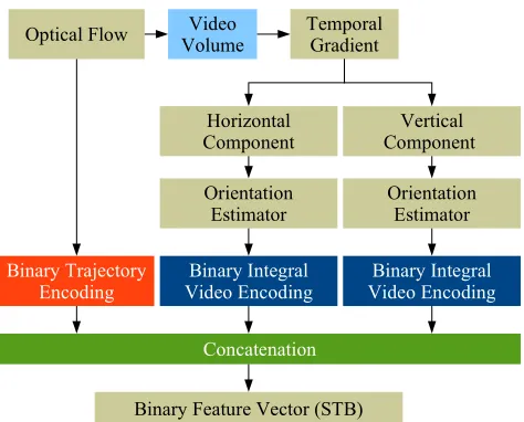
Fig. 1: STB descriptor. Each STSR, or video volume, is encoded as a concatenation of three binary strings: 1) BiTE encodes the video volume’s motion information extracted from optical flow. BIVE separately encodes the 2) horizontal and 3) vertical motion components of the temporal gradients.

of a video volume as a concatenation of three binary strings, as depicted in Fig. 1. The encoded motion information is obtained from two motion sources: optical flow and temporal gradients, which have been shown to provide rich motion information by considering pixel intensity changes to create a new data space that disregards the background [25]. The first binary string of STB represents the video volume’s motion information extracted from optical flow (see orange block – Binary Trajectory Encoding (BiTE) in Fig. 1). The second and third binary strings of STB represent the horizontal and vertical motion components of the video volume’s temporal gradients (see blue block – Binary Integral Video Encoding (BIVE) in Fig. 1). We detail next the computation of the binary strings comprising STB.

A. Binary Trajectory Encoding - BiTE

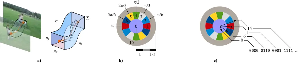
BiTE encodes the trajectories described by points tracked after computing the optical flow of the video data, e.g., by using the improved dense trajectory detector [34, 41]. The tra-jectory of each tracked point comprisesLdisplacement vectors representing motion information in time. Each trajectory, Ti, defines a STSR, or video volume,vi, of sizenx×ny×ntas Fig. 2.a illustrates. BiTE first normalizesTi with respect to its largest displacement vector to produceTˆi:

ˆ

Ti=

(∆pt, ...,∆pt+L−1)

maxk∆pk , (1)

a) b)

vi Ti

c)

ny

nx

nt

0

ε 1-ε π/6 π/3 π/2 2π/3

5π/6

π

15 1 2 3 4 5 6

0000 0110 0001 1111 … 06

115

Fig. 2: Binary Trajectory Encoding. a) A video volume, i.e., a STSR, is defined for each trajectory, which comprises L

displacement vectors. b) The direction and magnitude of the constituent displacement vectors are encoded using a binning stratregy. c)Example binning of 4 normalized displacement vectors.

codes, each representing a bin:

B(∆ˆpt) =



 

 

q: arg min_qk∆ˆpt−bq k :|∆ˆpt| ∈(,1−)

15dec :|∆ˆpt| ≥1−

0dec :|∆ˆpt| ≤

,

(2) wherebq is a unitary vector that represents the main direction associated with the qth bin. It is important to note that the binning strategy in Eq. 2 not only considers the direction of each displacement vector, but also their normalized magnitude. The latter is important to improve the descriptiveness power of the resulting binary codes because very small or very large displacements vectors tend to have unstable directions. Specifically, very small displacement vectors are prone to have random directions, while very large displacement vectors are likely to have been generated by camera motion. Eq. 2 then bins∆ˆpt into one ofQ= 6 binsif and only if its magnitude is within the range[,1−], which is the range of normalized magnitudes that captures the most stable directions. Those displacement vectors with normalized magnitudes ≤ are represented by the binary code 0000, or 0dec, while those with normalized magnitudes ≥1− are represented by the binary code1111, or15dec.

Table I tabulates the details of the Q = 6 bins used to encode the displacement vectors with normalized magnitudes ∈ [,1−], i.e., the stable displacement vectors. Note that compared with our previous work in [23], which employs shorter binary codes, by using 4-bit codes we can uniquely represent the six bins and use the most significant bit (MSB) to distinguish those very large, unstable displacement vectors, whose MSB is always 1. This increases the power of the descriptor to distinguish between stable and unstable dis-placement vectors. In order to make the encoding direction-invariant, the qth bin has a period of π. Fig. 2.b illustrates this concept, where the bins depicted in the same color are associated with the same binary string. Fig. 2.c illustrates the binning of 4 example normalized displacement vectors.

The binary vector,Fi, representing trajectoryTˆiis generated by concatenating theL binarized displacement vectors:

Fi=

X

06t<L

24tB(∆ˆpt). (3)

TABLE I: Bins used to encode the direction of stable displace-ment vectors.

Bin index (q) Main direction Binary string Range of directions

1 0 0001 ±π/12

2 π/6 0010 π/6±π/12

3 π/3 0011 π/3±π/12

4 π/2 0100 π/2±π/12

5 2π/3 0101 2π/3±π/12

6 5π/6 0110 5π/6±π/12

B. Binary Integral Video Encoding - BIVE

BIVE is based on our previous binary descriptor Binary Wavelet Differences (BWD) [23]. BIVE further improves the descriptiveness power of BWD by separately encoding the ver-tical and horizontal components of the STSR. Moreover, BIVE reduces the number of computations by using a technique based on IVs. BIVE comprises two main steps: 1) motion component calculation and 2) binary string formation, as Fig. 1 depicts.

1) Motion component calculation: To compute the hori-zontal and vertical motion components of vi , denoted byvix andv_iy, respectively, BIVE first applies a temporal difference operator dt = [−1,1] to discard background information. It then extracts vx

i and v y

i by applying the Prewit convolution operatorsdx= [−1,0,1]anddy = [−1,0,1]>, respectively:

v_ix=|dx∗(dt∗vi)|, (4a)

vy_i =|dy∗(dt∗vi)|. (4b) In order to make the binary string representing each compo-nent orientation-invariant, BIVE rotatesvx

i andv y

i. To this end, we extend the 2D Rosin operator [56] to the spatio-temporal domain to determine the components’ orientations. For each component, the coordinates of the centroid,c, are determined using the center of mass,m:

c= (m10

m00

,m01 m00

), (5a)

mpq=

X

16x6nx

X

16y6ny

X

16t6nt/2

xpyqvis(x, y, t), (5b)

Space – symmetric Time – symmetric

(1) (2)

(3) (4)

t y

x

r1

r2

r1 r2 _r

1

r2

r2

r1

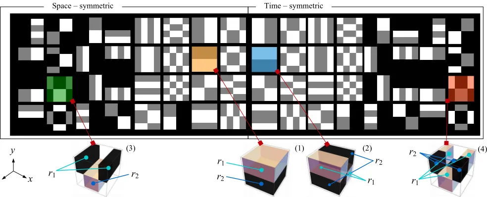
Fig. 3: Wavelet-based patterns. Each pattern defines two regions,r1 and r2. Four sample patterns are illustrated: (1) is complementary to (2), while (3) is complementary to (4).

geometric center, (nx/2, ny/2), the component’s orientation is given by the angle θof r=oc:

θ=atan2(ry, rx). (6)

Finally, θ is binned into four quadrant directions, i.e., θ ∈ {0, π/2, π,3π/2}, and vx

i and v y

i are rotated using the flip operation:

v_is(x, y, t) =

(

vs

i(x, ny−y, t), θ'π/2

v_is(nx−x, y, t), θ'0

. (7)

2) Binary string formation: BIVE separately encodes the horizontal and vertical motion components vx

i andv y i into a binary string. The encoding process is based on comparing the summed values of several pairs of relatively large regions defined within each motion component to create logical values. BIVE uses wavelet-based patterns to define the pairs of regions of vx

i and v y

i to be compared [20, 21, 57], which avoids seeking the best pairs, as required when using small isolated regions [18, 21]. Although it is possible to use other patterns, e.g., those used by FREAK [21], ORB [18] and DAISY [20], our evaluations show that other patterns provide inferior results than those provided by our wavelet-based patterns.

Fig. 3 depicts theK= 64patterns used by BIVE. Note that each pattern indeed divides a video volume into two regions, denoted byr1andr2. These patterns are symmetrical in either

space or time. For example, patterns (1) and (3) are space-symmetric while patterns (2) and (4) are time-space-symmetric. The difference between patterns (3)-(4) and (1)-(2) is that the latter pair contains void regions that are not considered during the encoding. Patterns with void regions reduce the overlap of the analysed STSR, which helps to produce very descriptive binary strings. Time-symmetric patterns are computed as the complement to space-symmetric patterns in the range[0, t/2]; e.g., (1) and (2), where (2) is complementary to (1). A pattern complementary to a symmetric one is therefore always time-symmetric and generated from a space-time-symmetric pattern.

It is important to note that the inclusion of time-symmetric patterns in this work is an important improvement compared to our previous work in [22, 23]. Time-symmetric and space-symmetric patterns allow fast and slow motion, respectively, to be captured thus improving the descriptiveness of the resulting binary strings compared to those in [23].

BIVE generates a bit by comparing the summed values of the two regions,r1_k andr_k2, generated by thekth pattern. This process is aK-dimensional mapping,R3→RK. The kth bit

for regions r_k1 andr_k2 is computed as follows:

C(r1_k, r2_k) =

(

1, if P _{v r}1 k

>P _{v r}2 k

0, otherwise , (8)

where P

(v(r_kn)) represents the summed values of region

n. BIVE then calculates a binary string, Gi, one for each motion component,v_ix andv_iy, as the concatenation of allK

comparisons:

Gi=

X

06k<K

2kC(r_k1, r_k2). (9)

Integral Video (IV): For the different K = 64 patterns in Fig. 3, Eq. 8 adds the same values several times, making the computation ofGihighly repetitive. To reduce the number of computations required by Eq. 8, BIVE uses the IV of each motion component as a way to pre-compute the summations. LetV_i,sp denote the IV of the motion componentsof volume

vi withs∈ {x, y}. Algorithm 1 details how to compute Vi,sp with a low complexity of O(n3_{) by adding the values ofv}s i up to pointp:

V_i,sp = X

1≤x≤xp

X

1≤y≤yp

X

1≤t≤tp

v_is(x, y, t), (10)

where(x, y, t)denote the coordinates ofvs_i. The values ofV_i,sp

at specific locations are then the summed values required by Eq. 8. For example, Fig. 4.b shows how to compare regionsr1

b

c

d

e _f

g h

(x0, y0, t0)

a

x y

t a

b

Va_{> V}b_{- V}a r1

r2

(x1, y1, t1) a1

b₁

a3

b4

a₂

b2

a4

b₃ b5

a₅

b8

a8

b6

a6

b7

a7

r₁

r2

a) b)

c)

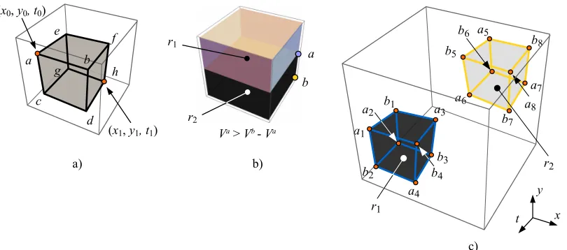
Fig. 4: a) Sub-volume defined by the eight pointsa−h. b) Comparing the summed values of regionsr1 and r2 requires one subtraction after computing the IV. c) Sets of points,A={a1, a2, ..., a8}andB={b1, b2, ..., b8}, defining two regions,r1 andr2, to be compared.

corresponding IV, i.e., Va _{and V}b_{, where} P _{v r}1 k

=Va

andP _{v r}2

k

= (Va_−Vb_).

Algorithm 1: Integral Video calculation

Input : motion componentvsi of size(nx, ny, nt), with s∈ {x, y}

Output : summed volumeVi,sp of size(xp, yp, tp)

Variables:accstores the summation ofvisup to location

(x, y, t)

vs

i is also used to store the summed values 1 acc= 0;

2 fort∈(1, tp)do 3 fory∈(1, yp)do 4 acc= 0;

5 forx∈(1, xp) do

6 acc=acc+v_is(x, y, t);

7 if y >1then

8 v_is(x, y, t) =acc+v_is(x, y−1, t);

9 continue

10 end

11 vis(x, y, t) =acc;

12 end 13 end

14 ift >1then

15 fory∈(1, yp)do 16 forx∈(1, xp) do

17 v_is(x, y, t) =vs_i(x, y, t) +v_is(x, y, t−1);

18 end

19 end 20 end 21 end

22 V_i,sp =vs_i(1 :xp,1 :yp,1 :tp)

Let us denote as A = {a1, a2, ..., a8} and B =

{b1, b2, ..., b8} the sets of points defining the two regions, r1

andr2, to be compared, as shown in Fig. 4.c. It can be easily

shown that Eq. 8 can be expressed as:

C(r1_k, r_k2) =

(

1, if VA k > VkB

0, otherwise , (11)

whereV_kA=Va1_+Va2_+...+Va8 _andVB

k =V

b1_+Vb2₊

...+Vb8_.

Eq. 11 has a O(n) complexity. For the K = 64 patterns depicted in Fig. 3, the size of A and B depends on the complexity of the regions. For instance, pattern (1) requires fewer points in A and B than pattern (4), and consequently, fewer operations to compute Eq. 11.

After computing the IVs for the two motion components,

vx i andv

y

i, a minimum of 24 Operations Per Bit (OPB), i.e., additions/subtractions, on average, are required to compute Eq. 11 for theK= 64patterns depicted in Fig. 3, with a maximum of 150 OPB, on average, regardless of the motion component’s size. On the contrary, when the IV technique is not used, the number of OPB depends on the motion component’s size, i.e.,

nx×ny×nt OPB.

The final STB descriptor forvi is the binary feature vector,

Hi, of dimensions D = 4L + 2K, that results from the concatenation of the binary string produced by BiTE (see Eq. 3), and the two binary strings produced by BIVE (Eq. 9), one for each motion component,vx

i andv y i:

Hi =Fi++Gxi ++G y

i. (12)

IV. FISHERVECTORS FOR BINARY DATA

We propose to pair our STB descriptor with FVs. Our FVs are based on the work of Uchida et al. [55]. However, we follow important assumptions introduced in the work of Perronin [51] to derive the Fisher Score and Information Matrix, as explained in Appendices A and B.

Let us denote the binary feature vector,Hi, as computed by Eq. 12, byxt. Thusxt∈ {0,1}Dis anD-dimensional binary feature. To generate the Bernoulli Mixture Model (BMM), let us define an input vectorX as comprising a total ofT binary features; i.e., X = {x1, x2, . . . , xT}. For an N-component BMM, we define the model’s distribution parameters as the set

across the dth dimension. The probabilistic density function for the T binary features inX is given as:

p(X|θ) = Y

16t6T

p(xt|θ), (13a)

p(xt|θ) =

X

16i6N

wipi(xt|θ), (13b)

pi(xt|θ) =

Y

16d6D

µxtd

id (1−µid)1−

xtd_{, (13c)}

wherextd represents thedth bit ofxt. The parameter setθis estimated using the Expectation Maximization (EM) algorithm [58]. Specifically, the expectation step calculates the posterior probability, γt(i) =p(i|xt, θ), of featurextgenerated by the

ith BMM component as follows:

γt(i) =

wipi(xt|θ)

P

16j6N

wjpj(xt|θ)

. (14)

In the maximization step, the parameters are updated as follows:

Si=

X

16t6T

γt(i), wi=Si/T, µid =

1

Si

X

16t6T

γt(i)xtd, (15) whereSiis the zero-order statistic. Parameterswiandµid are initialized to 1/N and a uniform distribution, U(1/4,3/4), respectively, as suggested in [55].

Once the parameters converge or the EM reaches a max-imum number of iterations, we proceed to map the features using the set of parameters, θ. Differently from the work by Uchida et al. [55], in this work we derive the FV from the BMM following the standard gradient derivation proposed in [51] with a Gaussian Mixture Model (GMM). This guarantees that the Information Matrix do not become undefined for small and large values of the distribution’s mean,µid.

A gradient vector describes the direction to which the parameters should be modified to best fit the data, X. Let us describeX by the gradientGX

θ , also known as Fisher Score:

GX

θ =

1

T∇θL(X|θ), (16a)

L(X|θ) = logp(X|θ). (16b) From Eq. 13a, and assuming independence over the BMM components, the Fisher Score can be expressed in terms of the distribution parameterµid (see Appendix A for derivation):

GX µid=

1

T

X

16t6T

γt(i)

Y

16d6D

xtd−µid

µid(1−µid)

. (17) Let us now consider a class of parametric models P(X|θ), where θ ∈ Θ defines the Riemannian manifold Mθ with

a local metric given by the Information Matrix F =

EX{GX GX >

}. The Fisher Score GX

θ mapsX into a new feature vector, i.e., X→ GX_{, which is a point in the gradient} space of the manifoldMθ. Specifically, the mapping is given by GX

θ = ∇θlogp(X|θ). The natural kernel, κ, of this mapping is the inner product between the Fisher Score relative to the local Riemannian metric of two sets of features,X and

Y:

κ(X, Y) =GθXFθ−1G Y

θ. (18)

The inner product defines an Euclidean metric that implicitly defines a pseudo-metric in the original feature space via a second-degree polynomial expansion of the kernel [59]. Therefore, the natural kernel is a strong similarity measure in the projected space based on the Euclidean distance. In this work, we calculate the Information Matrix required by Eq. 18 in terms of the distribution parameterµid as follows (see Appendix B for derivation):

Fµid=

T wi

µid−µ2id

. (19) The FV is a two-normalization of the score concatenationz=

Fµ1id/2G

X

µid. We first use power normalization with coefficient

α∈(0,1), as follows:

f(z) =sign(z)|z|α_.

(20)

We then normalizef(z)using `2 normalization [24] to

com-pute the final FV, i.e., Z =k f(z)k2. For an N-component

BMM of binary features withDdimensions, the FV hasN×D

dimensions as a result of the concatenation of the feature projections onto each individual BMM component.

It is important to mention three main differences between our FV formulation and that proposed by Uchida et al. [55]:

1) When deriving the Fisher Score (Eq. 17) and Informa-tion Matrix (Eq. 19), we do not consider the two possible values that the STB descriptor can take (i.e., 0or 1) to simplify the computations. Instead, we fully expand the expressions and compute the derivative (see Appendices A and B). This results in expressions that are much simpler to evaluate than those in [55]. Specially, the expressions of Uchida et al. [55] are:

GXµid= 1

T

X

16t6T

γt(i)

Y

16d6D

(−1)1−xtd

µxtd

id (1−µid)1−xtd

,

(21) and

Fµid =T wi

PN

j=1wjµjd

µ2 id

+

PN

j=1wjµjd

(1−µid) 2

!

. (22) 2) Our Information Matrix expression (Eq. 19) allows calculating the FVs without overflow. Specifically, when computing the product z =Fµ1id/2G

X

µid, it is easy to see

that the means in the denominators are to be multiplied. Because Eq. 22 generates smaller values than Eq. 19, the former is more prone to overflow for small values ofµid, i.e., when µid → 0. Our proposed Information Matrix is then more robust to this potential problem. In other words, Eq. 22 becomes undefined for small and large values of this mean. On the contrary, our Information Matrix is defined for a larger range of mean values (see Fig. 5).

3) Since µid is constant, all the denominators for Eq. 17 can be computed as:

βid =

1

µid(1−µid)

GX µid =

1

T

X

16t6T

γt(i)

Y

16d6D

βid(xtd−µid). (24) Compared to Eq. 21, our expression for the Fisher Score can then be computed without divisions, which gives gains in terms of processing speed.

μ_id F_μid

Fig. 5: Information Matrix per individual component as pro-posed in [55] (blue) and in this work (orange)

V. EXPERIMENTS ANDDISCUSSIONS

Five sets of experiments are conducted. The first set is aimed at confirming the descriptive power and low-dimensionality of BIVE. The second set compares the memory demands and computational time of STB with those of state-of-the-art non-binary and non-binary feature descriptors. The third set evaluates STB when paired with FVs for action recognition. The fourth set evaluates STB when paired with FVs for gait recognition and animal behavior clustering. The last set of experiments evaluates the effect of the FV parameters on the computational times and action recognition accuracy.

A. First set of experiments: BIVE performance

We evaluate the performance of BIVE against HOF [60], HOG [60], PCA-gradients [61], and several binary feature de-scriptors. Specifically, we compare it against motion FREAK (moFREAK) [50], the hashing techniques SSH, LSH [44, 45] and IQT [48], and a 3D version of FREAK, BRISK, ORB and BRIEF. The SSH, LSH, and IQT techniques map double-precision feature vectors to binary format. We apply these techniques to HOF features.

We extend FREAK, BRISK, ORB and BRIEF to the spatio-temporal domain by defining the pair of regions to be com-pared in 3D, as illustrated in Fig. 6. We call these extended 3D feature descriptors FREAK, BRISK, ORB and 3D-BRIEF, respectively. We employ the spatio-temporal detector of Laptev in [37], and a BoF+SVM pipeline. For the KTH dataset, we use the 8/9 split originally proposed by [62]. For the UCF50 dataset, we divide the 50 actions into 25 splits. The average CCR over the splits are reported in Tables II and III.

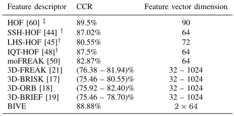
TABLE II: CCR for action recognition using various feature descriptors on the KTH dataset under a BoF+SVM pipeline

Feature descriptor CCR Feature vector dimension

HOF [60]‡ 89.5% 90

SSH-HOF [44]† _{87.02% 64}

LHS-HOF [45]† 80.55% 72

IQT-HOF [48]† _{87.5% 64}

moFREAK [50] 82.87% 64

3D-FREAK [21] (76.38 – 81.94)% 32 – 1024 3D-BRISK [17] (75.46 – 80.55)% 32 – 1024 3D-ORB [18] (75.92 – 82.40)% 32 – 1024 3D-BRIEF [19] (75.46 – 78.70)% 32 – 1024

BIVE 88.88% 2×64

† _{Binary mapping of double-precision feature vectors.} ‡ _{Double-precision feature vectors.}

TABLE III: CCR for action recognition using various feature descriptors on the UCF50 under a BoF+SVM pipeline.

Feature descriptor CCR Feature vector dimension

HOF [60]‡ 55.55% 90

HOG [60]‡ 52.45% 72

PCA-Gradients [61]‡ 53.06

-3D-FREAK [21] 42.76% 64

3D-BRISK [17] 41.82% 64

BIVE 54.25% 2×64

‡_{Double-precision feature vectors.}

From Tables II and III, we observe that BIVE attains the highest CCR among the evaluated binary feature descriptors. A major disadvantage of SSH, LHS and IQT is that they require that double-precision feature vectors, in this case HOF feature vectors, be computed first. Thus, besides the computational complexity of the binary-mapping, it is important to consider the multiple calculations and storage requirements to extract and store the double-precision feature vectors. BIVE signifi-cantly outperforms FREAK, BRISK, ORB and 3D-BRIEF. This confirms the advantages of using wavelet-based patterns and relatively large regions to encode the temporal gradients of video volumes.

When tested on a BoF+SVM pipeline, BIVE outperforms BiTE by 10% and 7% on the KTH and UCF50 datasets, respectively, in terms of CCR. When combined, BiTE+BIVE outperform BIVE by 6% and 14% on the KTH and UCF50 datasets, respectively. BiTE+BIVE also outperform BiTE by 15% and 20% on the KTH and UCF50 datasets, respectively This proves that BIVE is more powerful than BiTE and when used together, they provide a stronger performance than when used separately.

It is important to mention that FREAK, BRISK and ORB require finding the best pairs of regions to be compared. The particular criterion used by these 2D feature descriptors to find these best pairs of regions, unfortunately, gives preference to those pairs that tend to produce binary strings with a mean = 0.5, i.e., binary strings where half of the bits are

First Ring Second Ring Third Ring Combined y

x t

a) 2D FREAK patterns

b) 3D FREAK patterns

Fig. 6: Extension of the FREAK descriptor to 3D. a) Sample 2D FREAK patterns around a particular key point. Circular regions are progressively smaller as they are closer to the key point. b) 3D FREAK patterns defined in the spatio-temporal domain by using ellipsoids of three different sizes organized into three rings. The first ring (outermost layer) comprises the largest ellipsoids. The second and third rings comprise progressively smaller ellipsoids emulating the 2D FREAK patterns. The top row depicts the actual spatio-temporal regions to be compared, while the bottom row depicts the projected ellipsoids on the xytplanes for visualization purposes.

K CCR

40 50 60 70 80 90 100

0.80 0.82 0.84 0.86

1500 1200 800 400

2000

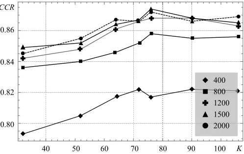
Fig. 7: CCR for the KTH dataset against K patterns for {400, . . . ,2000} centroids using a BoF+SVM pipeline.

preference to pairs of regions that tend to produce random binary strings, which defeats the purpose of creating highly descriptive feature vectors. In our experiments, we obtain more descriptive feature vectors for 3D-FREAK, 3D-BRISK and 3D-ORB by selecting those region pairs that produce strings whose mean are within the2σregion, whereσis the standard deviation. It is important to emphazise that BIVE employsK

patterns to define the pairs of regions to be compared and, therefore, does not require searching for the best pairs. In this work K = 64, which is a number of patterns that have been shown to provide the best trade-off between CCR and computational complexity. This is depicted in Fig. 7, where the CCR for the KTH dataset is plotted against K for a total of {400,800,1200,1500,2000} centroids using a BoF+SVM pipeline and a 8/9 split [62]. Note that for K >64 patterns, BIVE does not attain a significant increase in CCR values for any of the number of centroids evaluated.

B. Second set of experiments: STB complexity

This experiment compares the memory demands and com-putational time of the STB descriptor, with and without using the IV technique in BIVE, against several popular binary and non-binary feature descriptors. In this experiment, we use our 3D versions of FREAK and BRIEF. The results of this experiment are tabulated in Table IV, for a single video volume.

TABLE IV: Characteristics of various feature descriptors.

Feature descriptor Bytes per feature Computational time

3DSIFT [31] 18432 220 ms

MBH [34] 1728 100 ms

HOF [33, 60] 810 57 ms

HOG [33, 60] 640 43 ms

3D-FREAK† 4 – 128 (12 – 40) ms 3D-BRIEF† 8 – 128 (10 – 50)µs

STB (without IV)† 23 7.5 ms

STB (with IV)† 23 180µs

†_Binary.

From Table IV, we observe that using the IV technique indeed speeds up the encoding process by approximately40× compared to the case of not using it. We also observe that STB, when using the IV technique, is c.a. 1200×faster than 3DSIFT, and 200× faster than HOG. In terms of memory demands, feature vectors generated by STB are c.a. 830× more compact than those generated by 3DSIFT, and30×more compact than those generated by HOG. These results confirm the advantages of the proposed STB descriptor in terms of computational times and memory demands, as well as the benefits of using the IV technique to reduce the number of computations. A detailed analysis of the complexity of the STB descriptor is provided in Appendix C.

Optical Flow Feature Vectors _STB FV – BMM: Visual Fisher Vector _Mapping PCA nAkELM

X = ⋮ ⋮

101… 01

Σ

D×T

⋮

x1D xtD

xTD

⋮

⋮

γ1D γiD

γND

z1D×N

zPD×N ⋮

⋮

Z^k hn

Z=W Z^ f Z^k

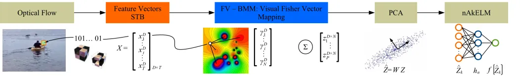
Fig. 8: Three-stage pipeline used to evaluate the proposed STB descriptor when paired with FVs. In the first stage, we extract STB feature vectors. The second stage projects the extracted binary feature vectors using FVs. In the last stage, the dimensions of the projected feature vectors are reduced using PCA; classification is done using an nAkELM.

hashing techniques SSH, LSH and IQT are applied to the IDT+MBH/HOG/HOF descriptor [34]. The compressed de-scriptors are tested on a BoF+SVM pipeline using the KTH dataset. The resulting CCRs are tabulated in Table V. As expected, applying a hashing algorithm reduces the amount of data needed to represent the feature descriptors, but may negatively affect the performance. Even after applying hashing techniques to IDT+MBH/HOG/HOF, our STB attains a very competitive CCR and has the lowest storage requirements.

TABLE V: CCR for the KTH dataset under a BoF+SVM pipeline using hashing techniques.

Descriptor Storage CCR

IDT+MBH/HOG/HOF [34] 5.85 GB 94.44% IQT-IDT+MBH/HOG/HOF (64 bits) 5.9 GB 92.45% SSH-IDT+MBH/HOG/HOF (64 bits) 5.9 GB 92.13% LSH-IDT+MBH/HOG/HOF (64 bits) 5.9 GB 86.11%

STB 40.9 MB 93.05%

C. Third set of experiments: action recognition

We pair our STB with our FVs (as computed in Section IV) in the pipeline depicted in Fig. 8, where the FVs are dimen-sionally reduced using PCA, as this has been shown to reduce noisy feature projections over the BMM components [64–66]. We employ first order-features for the FVs. The pipeline in Fig. 8 employs for classification an Nigstrom Approximation Kernel Extreme Learning Machine (nAkELM) [67] trained with the dimensionality-reduced FVs. This particular machine can be trained faster and has been shown to be more accurate than SVMs [67]. We use a greedy tuning to set the number of PCA components and the sample size and constraint factor of nAkELM [67].

1) UCF50: We compare STB+FV using the pipeline in Fig. 8 against several state-of-the-art action recognition methods that have been tested on the UCF50 dataset. Specifically, these methods are the best-performing ones that use high-order representations and double-precision feature vectors [6, 33, 34], double-precision feature vectors with no high-order representations [61, 68], and binary feature vectors [47]. The results of these comparisons are reported in Table VI, which correspond to the average CCR over the splits.

From Table VI, we observe that STB+FV achieves a very competitive performance compared to the best performing non-binary methods, outperforming GIST3D and c3DSIFT by c.a 10% and 15%, respectively. It is worth noticing

TABLE VI: CCR of various action recognition methods on the UCF50 dataset.

Method CCR

MIFS [6] 94.4%

IDT+MBH/HOF/HOG+FV [34] 91.2% DT/MBH/HOF/HOG+SVM [33] 84.5%

GIST3D [68] 73.7%

c3DSIFT [61] 68.2%

MIPs [47]† 72.70%

STB+FV† 83.05%

†_Binary.

that STB+FV is about 10% more accurate than MIPs. Even though STB+FV is about10%less accurate than the methdos in [6, 34], it is important to mention that these methdos usually require a long time, in the order of days, just to extract the feature vectors for this dataset. STB+FV requires approximately8.5 hours to extract the feature vectors for the whole UCF50 dataset and only3.3 GBto store them, which is significantly smaller than the846 GBrequired by the methods in [6, 34].

2) UCF101: We compare STB+FV using the pipeline in Fig. 8 against several state-of-the-art action recognition methods, including methods based on CNNs. To the best of our knowledge, no other method that employs binary feature descriptors has been tested on this dataset. We evaluate 1) the CNN methods proposed in [12, 69–74], 2) the method proposed in [34], which uses high-order representations and double precision feature vectors, and 3) the method presented in [75], which is among the best-performing ones that use double-precision feature vectors with no high-order repre-sentations. The results of this evaluation, in terms of the average CCR over the splits, are reported in Table VII. These results include the number of parameters of each method and the required hardware for operation. The evaluated methods are tabulated into two sections: the first section lists those that require GPUs, while the second section lists those that can operate on CPUs. From Table VII, we observe that STB+FV achieves a very competitive performance compared to some of the CNN methods. For example, STB+FV is only

TABLE VII: No. of parameters, hardware requirements and CCR of various methods for the UCF101 dataset.

Method Parameters Hardware CCR

Methods that require GPUs

I3D + PoTion [69] 25M+143M 65 GPUs 98.2%

Two-Streams I3D [70] 25M 32 GPUs 98%

DTPP [72] 12M+ 60.93M 3 GPUs 98%

RGB + OFF(RGB) + OFF(optical flow) + OFF(raw-OFF) [71]

44.2M 4 GPUs 96%

Two Stream-CNets [74] 25M GPUs∗ 88.8%

EMV-CNets [73] 32.8M 1 GPU 79.3%

MultiRes-CNets [12] 40.3M GPUs∗ 65.4%

Methods that require CPUs IDT/MBH/HOF/HOG+VLAN+FV

[34]

663.5K CPUs∗ 85.9%

H3D+HOF/HOG+SVM [75] 1.05M 1 CPU 43.9%

STB+FV† _{356.3K 1 CPU 71.6%}

†_Binary.

∗_{Arrays of GPUs or CPUs.}

of parameters and hardware requirements). For example, I3D + PoTion (25M+143M parameters) requires two pre-trained CNNs as feature generators. One CNN uses 3D convolutions (I3D) and is pre-trained on a large scale dataset of human actions (Kinetics dataset). The second CNN estimates human joints and is pre-trained on another large dataset (COCO dataset) using a frame-by-frame analysis. The Two-Streams I3D (25M parameters) and DTPP (12M+60.93M parameters) methods also require pre-training on a large scale dataset of human actions (Kinetics dataset). In contrasts, STB+FV has only356.3K parameters for the UCF101 dataset.

3) Binary pipeline: To further verify the superiority of STB against other binary feature descriptors, we also use the pipeline depicted in Fig. 8 to evaluate the accuracy of the hashing techniques IQT and SSH when applied to IDT+MBH/HOG/HOF [34]. We also evaluate BDT, which is the previous version of our binary feature descriptor [23]. In order to have a fair comparison, all descriptors are evaluated in conjunction with our FVs. It is important to recall that IDT+MBH/HOG/HOF is one of the best methods in terms of accuracy, as shown in Table VI. Specifically, we employ these descriptors in lieu of STB (orange block of Fig. 8) with exactly the same spatio-temporal detector. For the case of BDT, we replace STB (orange block of Fig. 8) with BDT and use the same spatio-temporal detector. BDT follows the same approach as that of STB, but produces shorter feature vectors of3L+Kdimensions, whereLis the number of displacement vectors andK the number of patterns, as defined before. For this evaluation, we compute the CCR for the UCF50 dataset. The results of this experiment are tabulated in Table VIII.

From Table VIII, we observe significant improvements of

STB of nearly 3% over SSH-IDT+MBH/HOG/HOF. STB

also outperforms IQT-IDT+MBH/HOG/HOF by nearly1%. In terms of storage requirements, STB drastically reduces storage requirements by 240×. Finally, STB requires a run time 5× shorter than that required by SSH-IDT+MBH/HOG/HOF and IQT-IDT+MBH/HOG/HOF. Compared to BDT, STB achieves a CCR value 4% higher. As expected, this improvement comes at the expense of longer run times and higher storage

TABLE VIII: Performance of binary feature descriptors on the UCF50 dataset.

Method Run Time Storage CCR

IQT-IDT+MBH/HOG/HOF+FV(64 bits) [48]

47.2 h 849.4 GB 82.12%

SSH-IDT+MBH/HOG/HOF+FV(64 bits) [44]

46.8 h 849.4 GB 80.56%

BDT+FV [23] 6.32h 2.43 GB 78.16 %

STB+FV 9.17h 3.29 GB 83.05%

requirements. Let us recall that BDT employs only three bits to binarize the trajectories and does not encode separately the two motion components of the video volumes. Consequently, the resulting binary feature vectors are shorter, but as shown in Table VIII, less powerful than those generated by STB.

D. Fourth set of experiments: gait recognition and animal behavior clustering

To demonstrate the generality of the STB descriptor, we also use the CASIA-B [76] and TIGdog [77] datasets for evaluation. For the CASIA-B dataset, we use the pipeline in Fig. 8. For the TIGdog dataset, we use the STB descriptor with FVs andk−means, as the objective is to cluster similar animal behaviors.

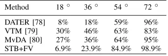
For the CASIA-B dataset, the performance is evaluated in terms of the recognition rate ([0,1]) for probe view angles [18◦,36◦,54◦,72◦]against the 90◦gallery view angle. In other words, training is done using exclusively 90◦data. The results of our STB descriptor and other methods are tabulated in Table IX. The STB descriptor outperforms the other evaluated methods for probe view angles [54◦, 72◦] by up to 20%, despite of the fact that STB is not specifically designed to deal with appearance transformations. It is worth mentioning that the other compared methods implicitly compensate for the angle variations, and thus attain a better performance for the most challenging cases, i.e., 18◦and 36◦angles. STB does not compensate for such variations. Instead, STB uses the raw videos to extract features, which also implies that there is no need to detect human silhouettes to compute the gait energy images commonly used in gait recognition. STB, consequently, simplifies this aspect of the gait recognition task. Overall, results in Table IX show that the STB descriptor is suitable for gait recognition.

TABLE IX: Gait recognition rates of various methods on the CASIA-B dataset.

Method 18◦ 36◦ 54◦ 72◦

DATER [78] 8% 18% 59% 96%

VTM [79] 30% 46% 63% 83%

MvDA [80] 27% 36% 64% 95% STB+FV 6.9% 23.9% 84.9% 98.9%

a) b) c)

32 64 128 256 N

Fitting Mapping

512 50

100 500 1000 5000

50k 256

128

64

0.8105

0.7791

0.7437 32

100k 250k 500k 1M 512

50k 256

128

64

32

100k 250k 500k 1M 512

12.6

6.33

2.65

N N

S

CCR

S

time(h)

time(s)

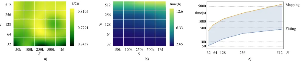
Fig. 9: FV parameter evaluation on split-1 of the UCF50 dataset. a) CCR for N BMM components fitting S STB feature vectors. b)Computational time of FV for N BMM components fittingS STB feature vectors. c)Computational time of the fitting and mapping processes of FV for N BMM components fittingS= 100k STB feature vectors.

by the total number of features. The ARI is similar to the purity, but penalizes the assignment of two features with the same label to different clusters. The results for the TIGdog dataset are tabulated in Table X. These results include the requirements to store the features extracted by each evaluated method and the time taken to extract the features. STB achieves a very competitive performance compared to other methods that employ double-precision features. Moreover, STB requires 140× less storage space than PoTs and IDT, and30×less storage than HOG. The time required to extract features is also reduced by nearly 6× and 4× compared to PoTs and IDT, and HOG, respectively.

TABLE X: Clustering performance of various methods on the TIGdog dataset.

Method Purity ARI Storage Feature extraction time

PoTs [77] 38 0.075 62.59 GB 5.12 h IDT [34] 37 0.05 62.59 GB 5.12 h HOG [60] 36 0.04 12.9 GB 3.48 h STB+FV 36 0.065 433.3 MB 0.88 h

E. Fifth set of experiments: FV parameter evaluation

For this last set of experiments, we employ split-1 of the UCF50 dataset. We compute the CCR attained by the pipeline depicted in Fig. 8 and the computational time of our FVs when a different number of BMM components are used with a different number of STB feature vectors. These are the most influential parameters of the computations of FVs.

We first use N BMM components withXS binary features to be fitted, where XS is a subset of X with S features randomly selected. The results of this experiment are shown in Fig. 9.a and 9.b. We observe that the CCR is particularly high for N > 64 BMM components and S > 250k STB feature vectors. As expected, computational times are also particularly high for N > 64 and S >250k (see Fig. 9.b). Experimentally, we find that S = 250k STB feature vectors usingN = 256BMM components is a good tradeoff between CCR and computational times. For these particular set of values, the computational time of FV is about 2.2 hours (see Fig. 9.b). Finally, Fig. 9.c plots the computational time of the fitting and mapping processes of FV forN BMM components fitting S = 100k STB feature vectors. From this Fig., we

can observe that mapping is indeed the process that takes the longest and has an exponential behavior with respect to the number of BMM components.

F. Discussions about computational complexity

Although some CNN methods and some methods based on double-precision feature vectors can attain higher CCRs than those attained by STB+FV, their training and operational times can be considerably long. CNN methods usually require dedicated clusters or servers with arrays of GPUs [74], and may require months for training [12]. The same drawback is shared by methods that employ double-precision feature vectors. Even when using dedicated servers, they may re-quire several days to process the extracted feature vectors [6, 34]. On the contrary, STB+FV takes only hours to process large datasets. For example, for the UCF101 dataset, it takes approximately 16 + 9 hours (see implementation details in Appendix D). Moreover, storing double-precision feature vectors demands a high number of resources. For example, the double-precision feature vectors used in [33, 34] require around 1.7 TB of storage for the UCF101 dataset, which is significantly larger than the 5 GB storage requirements of STB. Table XI summarizes the computational demands of STB and FV as paired in the pipeline of Fig. 8 when tested on a single CPU (see Appendix D). From this table, we can observe that STB and FV require significantly low computational resources for both UCF50 and UCF101.

TABLE XI: STB and FV computational demands

Dataset STB storage demands FV run time

UCF101 5.21GB 8.78h

UCF50 3.29GB 6.35h

connection weights, and applying Huffman encoding to the remaining quantized connection weights [82, 83]. However, even if compression is applied, the original CNN must be first fully trained, which still demands memory to store interme-diate feature maps and computational power to perform all operations. Moreover, pruning and weight quantization may affect the overall accuracy of the CNN [81].

Although GPU/TPUs can accelerate computing for methods based on CNNs, such computational power may not be avail-able in embedded applications, low-cost devices, or for large-scale operation, such as in the case of video surveillance using data from several cameras. Let us take the VGG-16 CNN as an example, which is widely used for image classification [84]. This CNN has over 138 million network parameters, which may require over 276 MB of memory space if a 16-bit number representation is used. Additionally, during operation, VGG-16 CNN produces several feature maps that must be stored internally in memory. Specifically, the largest feature map of the VGG-16 CNN is more than 6 MB. Since the VGG-16 CNN comprises 21 layers, the amount of data to be moved internally in memory may easily reach 60 MB. In terms of the number of operations, the VGG-16 CNN may need over 15G of multiply-accumulate (MAC) operations to classify one input image. Consequently, the deployment of CNNs in embedded applications and low-cost devices remains very challenging, especially when latency and throughput is a main concern.

The number of operations and memory requirements needed to extract and store the proposed STB descriptor are much lower than those of many CNN-based methods. Specifically, the number of operations and memory requirements of STB are, on average, linear and depend onn, the number of pixel locations of the spatio-temporal region, and theL, the number of displacements comprising each trajectory (see Appendix C for a detailed explanation). Moreover, the fact that the STB descriptor produces binary data allows performing subsequent computations using binary operators like AND and XOR, which further guarantees a low computational complexity. Combining hand-crafted binary feature descriptors, like STB, with low-complexity classifiers or low-complexity neural net-works (e.g., the nAkELM) is indeed an attractive solution for embedded applications and low-cost devices.

VI. CONCLUSIONS

In this work, we presented Spatio-Temporal Binarization (STB), a low-complexity and compact binary feature de-scriptor. STB encodes motion information from two sources, namely, optical flow and temporal gradients. Compared to our previous work, the performance of STB is improved in two aspects. First, it allows to distinguish motion information from motion camera and other small random movements. This is achieved by using longer binary codes to encode the constituent displacements of trajectories obtained from optical flow. Second, it allows to better describe the motion captured by temporal gradients by independently encoding the horizontal and vertical motion components. Furthermore, STB’s complexity is further reduced by employing a technique based on Integral Videos. Extensive evaluations for action

recognition, gait recognition and animal behavior clustering using the KTH, UCF50, UCF101, CASIA-B, and TIGdog datasets confirmed the advantages of STB in terms of pro-cessing times and storage requirements. These evaluations showed that when paired with the proposed Fisher Vectors for binary data, STB attains a very competitive accuracy, outperforming several state-of-the-art non-binary and binary features descriptors, including methods based on CNNs.

APPENDIXA FISHERSCORE

By substituting 13a into Eq. 16b, we have:

L(X|θ) = log



 Y

16t6T

p(xt|θ)



, (25a)

∵log(Y

k

ak) =

X

k

(log(ak)), (25b)

L(X|θ) = X

16t6T

log (p(xt|θ)). (25c)

The Fisher Score,GX

θ , can then be expressed as:

GX

θ =

1

T∇θ

X

16t6T

log (p(xt|θ)), (26a)

=1

T

X

16t6T

∂θlog (p(xt|θ)), (26b)

=1

T

X

16t6T

1

p(xt|θ)

∂θ(p(xt|θ)). (26c)

As [51] suggests, we derive the BMMµid parameter over the distribution and independence of wi from θ and not by only examining the two possible outcomes of xt, as done in [55]. We then have:

∂θp(xt|θ) =

X

16i6N

∂µid(wipi(xt|θ)), (27a)

= X

16i6N

wi∂µid(pi(xt|θ)). (27b)

We then estimate∂µid(pi(xt|θ))from Eq. 13c. At this point,

we fully expand the partial derivative and avoid simplifying the term only by its two possible values, as done in [55]:

∂µidpi(xt|θ) =

Y

16d6D

∂µid

µxtd

id (1−µid)1−

xtd_{. (28)}

Y

16d6D

∂µ µx(1−µ)1−x

, (29a)

Y

16d6D

x(1−µ)1−xµx−1−(1−x)(1−µ)−xµx, (29b) Y

16d6D

(1−µ)−x(x−µ)µx−1, (29c) Y

16d6D

µx(1−µ)1−x x−µ

µ(1−µ), (29d)

Y

16d6D

µxtd

id (1−µid) 1−xtd

| {z }

pi(xtd|θ)

Y

16d6D

xtd−µid

µid(1−µid)

, (29e)

∴∂µidpi(xt|θ) =pi(xtd|θ)

Y

16d6D

xtd−µid

µid(1−µid)

. (29f)

After substituting 29f in 27b, we have:

∂θp(xt|θ) =

X

16i6N

wipi(xtd|θ)

Y

16d6D

xtd−µid

µid(1−µid)

. (30) After substituting Eq. 14 in Eq. 26c, we finally have:

1

T

X

16t6T

1

p(xt|θ)

X

16i6N

wipi(xtd|θ)

| {z }

γt(i)

Y

16d6D

xtd−µid

µid(1−µid)

,

(31a)

∴GµXid= 1

T

X

16t6T

γt(i)

Y

16d6D

xtd−µid

µid(1−µid)

.

(31b)

APPENDIXB

FISHERINFORMATIONMATRIX

It can be shown that the first moment of the Fisher Score, i.e., its expected value, is 0. Thus the second moment, which corresponds to the Fisher Information, is given as follows:

Fµid=E

∂θL(X|θ)

2 |θ , (32a) = Z xt

p(xt|θ)

∂θlogp(X|θ)

2

dxt. (32b)

After simplifying the integration required by Eq. 32a, we have:

p(xt|θ)

∂θlogp(X|θ)

2

, (33a)

p(xt|θ)

X

16t6T

γt(i)

Y

1₆d₆D

xtd−µid

µid(1−µid)

!2

. (33b)

Assuming that the derivative of the posterior probability of

γt(i) is sharply peaked, we can simply write γt(i)2 ≈

γt(i),∀i. Unlike the work in [55], we derive the information matrix by assuming two separate integration terms and merg-ing them only when calculatmerg-ing it overT number of features. Then we have for xt:

Fµid=

Z

xt=0

. . . dxt+

Z

xt=1

. . . dxt. (34)

The sharply peaked derivative for the integrals is simplified as:

xtd−µid

µid(1−µid)

_x t=0

=− 1

1−µid

, (35a)

xtd−µid

µid(1−µid)

_x t=1 = 1 µid . (35b)

Therefore, we have two separate integration terms:

Fµid=

Z

xt=0

p(xt|θ)

X

16t6T

γt(i)2

(1−µid) 2dxt+

Z

xt=1

p(xt|θ)

X

16t6T

γt(i)2

µ2 id

dxt,

(36)

= X

16t6T

Z

xt=0

p(xt|θ)γt(i)

1

(1−µid) 2dxt+

X

1₆t₆T

Z

xt=1

p(xt|θ)γt(i)

1

µ2 id

dxt.

(37)

Considering thatp(xt|θ)γt(i) =wipi(xt|θ), Eq. 37 becomes:

Fµid=

X

16t6T

Z

xt=0

wipi(xt|θ)

(1−µid)2

dxt+

X

16t6T

Z

xt=1

wipi(xt|θ)

µ2 id

dxt.

(38)

After evaluating the integral, we have:

Fµid=

X

16t6T

wiµid

µ2 id

+ X

16t6T

wi(1−µid)

(1−µid)

2 , (39)

which finally leads to:

Fµid=T wi

₁

µid

+ 1

1−µid

, (40) or equivalently expressed using a single quotient:

Fµid=

T wi

µid−µ2id

. (41) Expression in Eq. 41 approximates the Fisher information ma-trix for a GMM [51]. Our information mama-trix is significantly simpler than that in [55], requiring one single term evaluation.

APPENDIXC

COMPLEXITY OF THESTBDESCRIPTOR

BiTE complexity: Let us recall that BiTE is computed by concatenating L binarized displacement vectors using Eq. 3, where each displacement vector,pˆt, is mapped into one of six 4-bit binary codes, using Eq. 2. BecauseB(∆ˆpt)in Eq. 2 can be calculated in linear time, the sum in Eq. 3 has a complexity ofO(n2). This complexity represents the worst case scenario, i.e., when it is necessary to calculate theLbinary codes using thearg min expression (if|∆ˆpt| ∈(,1−)) against Qbins, which results inQ×Loperations. For the best case scenario, either |∆ˆpt| ≥ 1− or |∆ˆpt| ≤ , the complexity is then

BiTE memory requirements: To compute Eq. 3, the trajectory and the Q bins must be stored. Each trajectory is made of 3 displacements, (x, y, t), thus 3n variables are required. The bins are stored as polar angles, thus requiring2Q

constants. Finally, we need to store each binarized trajectory, which requires 4n variables. The total memory requirements are then 7n+ 2Qper BiTE feature.

BIVE complexity: To compute BIVE, the horizontal and vertical motion components of volume vi must be computed first using Eq. 4a and 4b. Since two gradients are applied to compute each component, Eq. 4a and 4b require each

2n operations for the n pixels locations of vi. For each component, determining the coordinates of the centroid, c, requires multiplying the value of every pixel location by its location, which can be computed in n operations, according to Eq. 5. Computing the angle θ requires only one operation (see Eq. 6). The flip operation requires to re-allocate n

pixels locations, thus n operations are required (see Eq. 7). Calculating the Integral Video, as described in Algorithm 1, can be computed with n accumulations for n pixel locations (see Eq. 10). Finally, for thekth pattern, the expression in Eq. 11 must be evaluated.

For theK= 64patterns used in this work, 1056 operations are required for each video component, with an average of 150 OPB (or pattern). If the flip operation is required, which represents the worst case scenario, the total number of operations for the n pixel locations of video volumevi is

2(4n+ 1056 + 1). For the best case scenario, i.e., when no flip operation is required, the total number of operations is

2(3n+ 1056 + 1). Thus, the complexity of BIVE isO(n)for

n pixel locations.

BIVE memory requirements:Given the npixel locations of video volume vi, the memory requirements are2nfor the two components. When evaluating the Integral Video, the same memory spaces assigned to the video volume vi are used in the recursive operation, thus no additional memory is required. The total memory requirements of BIVE are then 2n+ 2K

for K patterns.

APPENDIXD IMPLEMENTATIONDETAILS

We implement STB+FV (pipeline in Fig. 8) in MATLAB and perform evaluations on a single 2.7GHz CPU with 16GB RAM memory. We use the homogeneous patch detector pro-posed in [34] as implemented by the authors. Video volumes used by STB are of size nx = 32, ny = 32, nt = 15. For BiTE, we use = 0.1 to encode the displacement vectors. We use the nAkELM implementation provided by the authors [67]. For evaluations on the KTH dataset, we use the STIP detector as implemented by the authors of [37] and the χ2

-SVM as implemented by the corresponding authors1. The size of the video volumes used in Section V-A are nx=ny = 9σ and nt = 9τ, where σ and τ are the scales at which the corresponding STIP is detected.

1_{https://goo.gl/chhfq0}

REFERENCES

[1] Cisco, “Cisco visual networking index: Forecast and methodol-ogy, 2014-2019 white paper,” https://goo.gl/xoBrTA.

[2] O. Popoola and K. Wang, “Video-based abnormal human be-havior recognition;a review,” IEEE Transactions on Systems, Man, and Cybernetics, Part C: Applications and Reviews,2012, vol. 42, no. 6, pp. 865–878, Nov 2012.

[3] H. Nam and C. D. Yoo, “Content adaptive video summarization using spatio-temporal features,” in 2017 IEEE International Conference on Image Processing (ICIP), Sept 2017, pp. 4003– 4007.

[4] J. Wang, W. Wang, and W. Gao, “Multi-scale deep alternative neural network for large-scale video classification,”IEEE Trans-actions on Multimedia, pp. 1–1, 2018.

[5] J. Zheng, X. Cao, B. Zhang, X. Zhen, and X. Su, “Deep ensemble machine for video classification,”IEEE Transactions on Neural Networks and Learning Systems, pp. 1–13, 2018. [6] Z. Lan, M. Lin, X. Li, A. G. Hauptmann, and B. Raj, “Beyond

gaussian pyramid: Multi-skip feature stacking for action recog-nition,” inComputer Vision and Pattern Recognition (CVPR), 2015 IEEE Conference on, June 2015, pp. 204–212.

[7] L. Wang, Y. Qiao, and X. Tang, “Action recognition with trajectory-pooled deep-convolutional descriptors,” inComputer Vision and Pattern Recognition (CVPR), 2015 IEEE Conference on, June 2015, pp. 4305–4314.

[8] H. Dee and S. Velastin, “How close are we to solving the problem of automated visual surveillance?” Machine Vision and Applications, vol. 19, no. 5-6, pp. 329–343, 2008. [9] N. Haering, P. Venetianer, and A. Lipton, “The evolution

of video surveillance: an overview,” Machine Vision and Applications, vol. 19, no. 5-6, pp. 279–290, 2008.

[10] Y. Cong, J. Yuan, and J. Liu, “Abnormal event detection in crowded scenes using sparse representation,” Pattern Recognition, vol. 46, no. 7, pp. 1851 – 1864, 2013.

[11] R. Leyva, V. Sanchez, and C. T. Li, “Video anomaly detection with compact feature sets for online performance,”IEEE Trans-actions on Image Processing, vol. 26, no. 7, pp. 3463–3478, July 2017.

[12] A. Karpathy, G. Toderici, S. Shetty, T. Leung, R. Sukthankar, and L. Fei-Fei, “Large-scale video classification with convolu-tional neural networks,” in2014 IEEE Conference on Computer Vision and Pattern Recognition, June 2014, pp. 1725–1732. [13] M. Bilal, A. Khan, M. U. K. Khan, and C. M. Kyung, “A

low-complexity pedestrian detection framework for smart video surveillance systems,”IEEE Transactions on Circuits and Sys-tems for Video Technology, vol. 27, no. 10, pp. 2260–2273, Oct 2017.

[14] T. Ojala, M. Pietikainen, and T. Maenpaa, “Multiresolution gray-scale and rotation invariant texture classification with local binary patterns,” Pattern Analysis and Machine Intelligence, IEEE Transactions on, vol. 24, no. 7, pp. 971–987, Jul 2002. [15] S. Saha and V. Demoulin, “Aloha: An efficient binary descriptor

based on haar features,” inImage Processing (ICIP), 2012 19th IEEE International Conference on, Sept 2012, pp. 2345–2348. [16] Y. Ma and P. Cisar, “Event detection using local binary pat-tern based dynamic textures,” inComputer Vision and Pattern Recognition Workshops, 2009. CVPR Workshops 2009. IEEE Computer Society Conference on, June 2009, pp. 38–44. [17] S. Leutenegger, M. Chli, and R. Siegwart, “Brisk: Binary robust

invariant scalable keypoints,” inComputer Vision (ICCV), 2011 IEEE International Conference on, Nov 2011, pp. 2548–2555. [18] E. Rublee, V. Rabaud, K. Konolige, and G. Bradski, “Orb: An efficient alternative to sift or surf,” inComputer Vision (ICCV), 2011 IEEE International Conference on, Nov 2011, pp. 2564– 2571.