ALEA: A Fine-grained Energy Profiling Tool
Lev Mukhanov, Queen’s University of Belfast Pavlos Petoumenos, University of Edinburgh Zheng Wang, Lancaster University
Nikos Parasyris, Queen’s University of Belfast
Dimitrios S. Nikolopoulos, Queen’s University of Belfast Bronis R. de Supinski, Queen’s University of Belfast Hugh Leather, University of Edinburgh
Energy efficiency is becoming increasingly important, yet few developers understand how source code changes affect the energy and power consumption of their programs. To enable them to achieve energy savings, we must associate energy consumption with software structures, especially at the fine-grained level of functions and loops. Most research in the field relies on direct power/energy measurements taken from on-board sensors or performance counters. However, this coarse granularity does not directly provide the needed fine-grained measurements. This article presents ALEA, a novel fine-grained energy profiling tool based on probabilistic analysis for fine-grained energy accounting. ALEA overcomes the limitations of coarse-grained power-sensing instruments to associate energy information effectively with source code at a fine-grained level. We demonstrate and validate that ALEA can perform accurate energy profiling at various granularity levels on two different architectures: Intel Sandy Bridge and ARM big.LITTLE. ALEA achieves a worst case error of only 2% for coarse-grained code structures and 6% for fine-grained ones, with less than 1% runtime overhead. Our use cases demonstrate that ALEA supports energy optimizations, with energy savings of up to 2.87 times for a latency-critical option pricing workload under a given power budget.
CCS Concepts:rHardware→Power and energy;rSoftware and its engineering→Software nota-tions and tools;
Additional Key Words and Phrases: Energy profiling, sampling, energy efficiency, power measurement, ALEA
1. INTRODUCTION
In an era dominated by battery-powered mobile devices and servers hitting the power wall, increasing the energy efficiency of our computing systems is of paramount im-portance. While performance optimization is a familiar topic for developers, few are even aware of the effects that source code changes have on the energy profiles of their programs. Therefore, developers require tools that analyze the power and energy con-sumption at the source-code level of their programs.
Prior energy accounting tools can be broadly classified into two categories: tools that directly measure energy using on-board sensors or external instruments [Chang et al. 2003; Flinn and Satyanarayanan 1999; Ge et al. 2010; Kansal and Zhao 2008; Keranidis et al. 2014; McIntire et al. 2007]; and tools that model energy based on activity vectors derived from hardware performance counters, kernel event counter-s, finite state machinecounter-s, or instruction counters in microbenchmarks [Bertran et al. 2013; Manousakis et al. 2014; Contreras and Martonosi 2005; Isci and Martonosi 2003; Curtis-Maury et al. 2008; Shao and Brooks 2013; Tsoi and Luk 2011; Tu et al. 2014;
Extension of Conference Paper: A preliminary version of this article entitled “ALEA: Fine-grain Energy Profiling with Basic Block Sampling” by Lev Mukhanov, Dimitrios S. Nikolopoulos and Bronis R. de Supinski appeared in International Conference on Parallel Architectures and Compilation Techniques(PACT), 2015. Permission to make digital or hard copies of part or all of this work for personal or classroom use is granted without fee provided that copies are not made or distributed for profit or commercial advantage and that copies bear this notice and the full citation on the first page. Copyrights for third-party components of this work must be honored. For all other uses, contact the owner/author(s).
c
YYYY Copyright held by the owner/author(s). 1544-3566/YYYY/01-ARTA $15.00
Wilke et al. 2013; Pathak et al. 2012; Schubert et al. 2012]. All of these tools can associate energy measurements with software contexts via manual instrumentation, context tracing, or profiling. However, these approaches have their limitations.
Direct power measurement:Using direct power measurement instruments, tools can
accurately measure hardware-component-level and system-wide energy consumption. State-of-the-art external instruments such as the Monsoon power meter [Brouwers et al. 2014], direct energy measurement and profiling tools [Ge et al. 2010; Flinn and Satyanarayanan 1999], and internal energy and power sensors such as Intel’s Run-ning Average Power Limit (RAPL) [Rotem et al. 2012] or on-board sensors [Cao et al. 2012] sample at a rate between 1 kHz and 3.57 kHz. This rate is unsuitable for ener-gy accounting of individual basic blocks, functions, or even longer code segments that typically run for short time intervals. Thus, we cannot characterize the power usage of these fine-grained code units and will miss many optimization opportunities that can only be discovered through fine-grained energy profiling.
Activity-vector-based measurement: Tools that model energy consumption from
ac-tivity vectors extracted from hardware performance counters can produce estimates for fine-grained code units but suffer from several shortcomings. Their accuracy is architecture- and workload-dependent [Curtis-Maury et al. 2008; Contreras and Martonosi 2005; Isci and Martonosi 2003; Schubert et al. 2012]. Thus, they are on-ly suitable for a limited set of platforms and applications. Further, targeting a new platform or workload requires expensive benchmarking and training to calibrate the model. Finally, as we show later, these tools are not accurate enough to capture the power variation caused by the execution of different code regions.
To overcome the limitations of prior work, this paper presents ALEA, a new proba-bilistic approach for estimating power and energy consumption at a fine-grained lev-el. Specifically, we propose a systematicconstant-power probabilistic model(CPM) to estimate the power consumption of coarse-grained code regions with latency greater than the minimum feasible power-sensing interval and an improved variation-aware
probabilistic model(VPM) that estimates power more accurately by identifying
high-frequency variations at the fine-grained level through additional profiling runs. CPM approximates the power consumption of a region under the assumption that power is constant between two successive readings of the system’s power sensors. Its accu-racy depends on the minimum interval that is allowed between two such readings. VPM relaxes this assumption and identifies power variation over intervals significant-ly shorter than the minimum feasible power-sensing interval. We validate CPM by comparing the results of profiling with real energy measurements on two different architectures using a set of diverse benchmarks. The experimental results show that CPM is highly accurate, with an average error below 2% for coarse-grained regions. However, for fine-grained regions this model can produce much higher errors. VPM successfully handles these cases, allowing energy accounting at a frequency that is up to two orders of magnitude higher than on-board power sensing instruments, with the error of its estimates at 6%, which is 92% lower than those of CPM.
Finally, we present two use cases of ALEA: fine-grain memoization in financial op-tion pricing kernels to optimize performance under power caps; and fine-grained DVFS to optimize energy consumption in a sequence alignment algorithm. These use cases show that our approach can profile large real-world software systems to understand the effect of optimizations on energy and power consumption.
The contributions of this paper are:
— Two first-of-their-kind, portable probabilistic models for accurate energy accounting of code fragments of granularity down to 10µSec, or two orders of magnitude finer than direct power measurement instruments;
— Low-latency and non-intrusive implementation methods for fine-grained, online en-ergy accounting in sequential and parallel applications;
— Tangible use cases that demonstrate energy efficiency improvements in realistic ap-plications, including energy reduction by 2.87×for an industrial strength option pric-ing code executed under a power cap and up to 9% reduction in energy consumption in a sequence alignment algorithm.
The rest of this paper is structured as follows. Section 2 provides a short overview of our profiling approach. Section 3 details our energy sampling and profiling models, while Section 4 examines the key aspects of their implementation. Section 5 demon-strates the accuracy of the proposed probabilistic models. Section 6 details opportu-nities and limitations of ALEA, including the effect of hysteresis on physical power measurements and an analysis of ALEA’s accuracy compared against power models based on hardware performance counters. Section 7 presents how ALEA can be used to improve energy efficiency in realistic applications. Section 8 discusses previous work in this area and Section 9 summarizes our findings.
2. OVERVIEW OF ALEA
ALEA provides highly accurate energy accounting information at a fine granularity to reason about the energy consumption of the program. It collects power and perfor-mance data at runtime without modifying the binary. ALEA uses probabilistic models based on its profiling data to estimate the energy consumption of code blocks.
2.1. Definitions
We define terms that we use throughout the paper as follows:
—Code block: a region of code that the user defines at the final profiling stage and that can include one or more basic blocks or procedures;
—Sampling interval:the time between two consecutive samples;
—Power-sensing interval:the interval during which a single power measurement is taken in a computing system;
—Fine-grained block:a code block that has an average latency less than the power-sensing interval;
—Coarse-grained block: a code block that has an average latency of at least the power-sensing interval.
2.2. Workflow
Figure 1 illustrates the three steps of the ALEA workflow:
Profiling. The instrumented program is profiled using several representative input
data sets. During each run, ALEA periodically samples instruction addresses and records readings from a power measurement instrument such as an on-board ener-gy sensor or a software-defined power model (e.g., based on hardware counters).
Disassembling and parsing.After each run, ALEA disassembles the binary and
i-dentifies basic blocks in the code.
Energy accounting.As we show in Section 5, the default model of ALEA (CPM, see
ALEA Application
Run
Profile
ALEA
Diassemble
Application
Parse
Collect
Basic Blocks
Collect
Data
A
LE
A Application
Assign
on
-li
n
e
of
f-lin
e
off-line
1
2
3
Fig. 1. Workflow of ALEA
of the power sensors and provides accurate energy estimates over intervals with la-tency down to 10µs. Finally, ALEA probabilistically estimates the execution time and power consumption of each code block.
3. ENERGY ACCOUNTING BASED ON A PROBABILISTIC MODEL
This section details our probabilistic energy accounting models. We first present our execution time profiling method in Section 3.1, followed by our sampling method in Section 3.2. We then describe our constant and variation-aware power models in Sec-tion 3.3. We extend our methodology to multi-threaded code in SecSec-tion 3.4. We close this section with an analytic study of the accuracy of our energy accounting models.
3.1. Execution Time Profiling Model
Our execution time profiler randomly samples the program counter multiple times per run. Based on the total execution time of the program and the ratio of samples of a code block to the total number of samples, we estimate the time that a block executes. More formally, we define a processor clock cycle as a unit of the finite population (U). It has been demonstrated that the execution time of code blockblmcan be estimated based on the probability to sample this block at a random cycle [Mukhanov et al. 2015; Graham et al. 1982]:
ˆ
tblm= ˆpblm·texec =nblm·texec
n (1)
In Equation (1)tblmis the the total execution time estimate of instances ofblm,texec is
[image:4.612.183.431.101.322.2]500 1000 1500 2000
Time, 10−1 ms
1.0 1.2 1.4 1.6 1.8 2.0 2.2 2.4 2.6
Power, W
start power measurements
sampling point
power of blm
idle power
stop power measurements
code block blm
(latency
blm)power-sensing interval
t
avr pow
(pow
blmi)
Fig. 2. Power measurements for CPM
3.2. Systematic Sampling
We use systematic sampling, which approximates random sampling. It selects the first sample (unit) randomly from the bounded interval[1, length of sampling interval]and other samples are selected from an ordered population with an identical sampling interval. We subsequently sample in the same run everysampling intervalclock cycles. The random selection of the first sample ensures that sampling is sufficiently random. Even if the sampling interval aligns with a pattern in the execution of the program, we can still obtain accurate estimates by aggregating multiple profiling runs, each one with a different initial sampling time.
3.3. Probabilistic Power Models
We apply the same probabilistic approach that we use for time profiling in order to profile power and energy. We consider power consumption as a random variable that follows a normal distribution and is a characteristic associated with the clock cycle population. We simultaneously sample the program counter and power consumption, which we assign to the sampled code block.
Assumingnblmsamples of blockblm, we estimate its mean power consumption as:
d
powblm= 1 nblm
·
nblm
X
i=1
powblmi (2)
wherepowi
blmis the power consumption associated with theith sample of blockblm.
We estimate the energy consumption ofblmas:
ˆ
eblm=powdblm·ˆtblm (3)
[image:5.612.190.408.108.273.2]100 200 300 400 500 600 700 1.0
1.5 2.0 2.5 3.0
Power, W
sampling
point
idle power
pow
idleaverage power
pow
no_delayA→C
A
B
B
0C
first
blminstruction
↓
last
blminstruction
↓
2100 2200 2300 2400 2500 2600 2700 Time, µSec
1.0 1.5 2.0 2.5 3.0
Power, W
sampling
point
delay
latency
blmaverage power
pow
delayA→C(delayed sample)
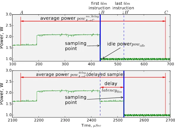
Fig. 3. Power measurements for VPM
3.3.1. Constant Power Model. Figure 2 shows an example of the power measurement
process of our Constant Power Model (CPM). When we sample the instruction pointer (the blue line), we interrupt the profiled threads, which causes the power consumption to drop quickly to the idle state, where it stays while all threads are paused. If we then measure power, this behavior would impact our measurement significantly. Thus, we measure power before sampling the current instruction pointer.
This model provides accurate power estimates for coarse-grained blocks. Howev-er, the power-sensing interval necessarily adjusts power consumption for other code blocks with potentially different power behavior. CPM, as well as all other existing energy profiling approaches, assumes that power remains constant throughout the power-sensing interval. If the power level varies during this interval, these energy profiling techniques do not capture that power variation.
3.3.2. Variation-Aware Power Model.Accurately measuring power for fine-grained code
blocks requires a more sophisticated approach, which ourVariation-aware Power Mod-el(VPM) provides. We isolate each block’s power consumption from that of the neigh-boring code blocks through multiple power measurements for the exact same se-quences of code blocks. By pausing (or not) the execution of the last block in this sequence, we control whether it contributes (or not) to the power measurement. We subtract the power associated with a sequence that omits the block from that of one that includes it to obtain the power and energy consumption of that block.
The top plot in Figure 3 shows this process in more detail. VPM partially decouples measuring power from sampling. We initiate the power measurement at pointAin the plot. The actual sample is taken after a certain amount of time, at pointB. Sampling causes the program to pause, bringing the power consumption down topowidle. At the
end of the power-sensing interval, pointC, we obtainpowAno delay→C .
[image:6.612.159.452.91.306.2]The bottom half of Figure 3 shows that this delay causes half of the samples that would be taken at Bto be taken atB’ (blm’s end). The power-sensing interval covers the same preceding blocks as in the case of sampling atBbut also includesblm. The difference of the two power readings gives us the energy and power consumption of
blm:
eiblm=powdelayA→C·tavrpow−powno delayA→C ·tavrpow+powidle·latencyblmi . (4)
powiblm=pow delay A→C−pow
no delay A→C latencyi
blm
·tavrpow+powidle, (5)
where powAdelay→C denotes the power measurements taken when we sample the last in-struction of blmatB’, powno delayA→C denotes power measurements taken when the first instruction of the code block was sampled atB,powidle is the idle power consumption obtained after interrupting the profiled threads andtavr
powis the power-sensing interval.
Our approach assumes that the power readings correspond to observations of a ran-dom variable with a normal distribution. Thus, we can averagepowdelayA→CandpowAno delay→C
over all samples to estimate the power consumption forblmas:
d
powblm=powd
delay A→C−powd
no delay A→C
d
latencyblm ·t avr
pow+powidle, (6)
wherelatencyd blmis the average latency of the code block.
For VPM to produce accurate results, all power readings associated with the same sample, delayed or not, must cover the power consumption of the same code blocks. The time between the start of the power measurement and the sampling point must be constant, as must the time between the sampling point and the end of the measure-ment. We carefully implement VPM to meet these requirements as much as possible. The only source of error that we cannot control is variations of the execution path and the power consumption before the targeted code block. Given the regular nature of most applications, these variations are not a significant source of error. In Section 5.2 we validate VPM and we show that it accurately estimates power consumption.
If the latency of profiled code blocks is small enough then the accuracy of power sen-sors could be insufficient to evaluate the difference betweenpowddelayA→C and powdno delayA→C
(see Section 5.3). VPM may obtain erratic power measurements due to insufficient accuracy of the power sensors. To overcome this problem, we force upper and lower bounds on VPM power readings to correspond to the peak power consumption of the processor andpowidlerespectively.
3.4. Multi-threaded Code
Multi-threaded applications execute many code blocks in parallel on different cores. To profile applications running on the same processor package at the code block level, we define a vector of code blocks that execute in parallel on different cores as:
−−→
blm=blmthr1, blmthr2, . . . , blmthrl. (7)
We use the same time and energy profiling models as in sequential applications. The only difference is that we associate multi-threading samples with vectors of code blocks. We distribute the execution time and energy across code block vectors as:
ˆ t−−→
blm= ˆp−blm−→·texec= n−−→
blm·texec
Code blocks
core1:cb100,core2:cb100 core1:cb100,core2:sys core1:cb161,core2:cb161
Samples
163 94 91
Time
21.99 +/‐0.44
0.95 +/‐0.19
0.92 +/‐0.18
Energy
67.95 +2.71/‐2.65
1.66 +0.42/‐0.39
2.29 +0.54/‐0.51
Power
3.09 +/‐0.06
1.75 +/‐0.08
2.48 +/‐0.07
Fig. 4. Profiling results for theheartwallbenchmark on the Exynos platform
d
pow−−→
blm= 1 n−−→
blm
·
n−−→
blm
X
i=1
pow−i−→
blm. (9)
We examine all running threads collectively during sampling, because they share re-sources. Such shared resources include caches, buses, and network links, all of which can significantly increase power consumption under contention. We could apportion power between threads based on dynamic activity vectors that measure the occupan-cy of shared hardware resources per thread [Manousakis et al. 2014]. However, these vectors are difficult to collect and to verify as current hardware monitoring infrastruc-tures do not distinguish between the activity of different threads on shared resources. Figure 4 shows the results of profiling the heartwall benchmark (Rodinia suite) on the Exynos platform (see Section 4.1), including 95% confidence intervals for each estimate.core1:cb100,core2:cb100denotes the code block with identification100 ex-ecuted simultaneously on the first and second cores. Similarly,cb161is the code block with identification161andsysis a code block from thepthread cond wait()function of the glibc library; it executes amutex lock that keeps a core in sleep mode until the corresponding(pthread cond signal) occurs. We see thatcb100executed in paral-lel consumes almost twice as much power than when it is co-executed with the sys
block. In the second case, the second core is sleeping and consumes almost no power. The difference in power consumption between parallel execution of cb161and cb100
is related to the cache access intensity of these blocks. Our earlier work shows that dynamic power consumption grows with this intensity [Mukhanov et al. 2015].
The number of sampled code block vectors depends on the number of code blocks in a parallel region and it grows exponentially with the number of cores. Thus, for high-ly parallel regions containing multiple code blocks, the number of code block vectors could render the analysis of profiling results slow, since we should account for the en-ergy consumption of all vectors. In practice and in all applications with which we have experimented, strong temporal locality of executing code blocks keeps the number of vectors of code blocks that execute concurrently (and, thus, are sampled) low. For ex-ample, inheartwall, three code block vectors dominate energy consumption (Figure 4), while the total number of sampled code block vectors is about 100 in this benchmark.
3.5. Analysis of Model Accuracy and Convergence
ALEA provides confidence intervals for its time, power, and energy estimates. We have shown in earlier work [Mukhanov et al. 2015] how to construct confidence intervals for the time and CPM power estimates.
Using the confidence intervals for execution time and power, we can also evaluate the worst case upper and lower bounds for energy consumption:
ˆ tl−−→
blm·powd
l
−−→
blm≤e−blm−→≤ˆt u
−−→
blm·powd
u
−−→
blm. (10)
whereˆtl
−−→
blm( ˆ tu
−−→
blm) is the lower (upper) bound of the confidence interval for the time
esti-mates andpowdl−−→
blm(powd
u
−−→
blm) is the lower (upper) bound of the power confidence interval.
[image:8.612.128.490.93.142.2]ex-0 1000 2000 3000 4000 5000 Number of samples 16.6
16.8 17.0 17.2 17.4
Execution time, Sec
0 1000 2000 3000 4000 5000 Number of samples 8.0
8.1 8.2 8.3 8.4 8.5 8.6 8.7
En
er
gy
,
10
3 J
0 1000 2000 3000 4000 5000 Number of samples 4.6
4.7 4.8 4.9 5.0 5.1
Po
we
r,
10
2 W
estimated time/energy/power measured time/energy/power
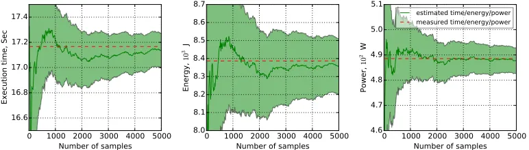
Fig. 5. Estimated vs. measured execution time, energy and CPM power for a code block ofheartwall(Sandy Bridge)
ecution time. We can increase the number of samples of each code block to narrow the confidence interval for power estimates. Thus, to narrow both confidence intervals, we can increase the total number of samples and the number of samples per block.
To demonstrate the accuracy improvements of our time, energy and CPM power estimates as the number of samples increases, Figure 5 shows their evolution for a coarse-grained code block from theheartwallbenchmark. We run this benchmark on our Sandy Bridge server (see Section 4.1). The dark green line represents the time (left), energy (middle) and power (right) estimates, whereas the lighter green area shows the 95% confidence interval for each estimate. The red dashed line in each plot corresponds to direct measurements for the block averaged over several runs.
The minimum number of samples for the block, collected during the first run of the experiment, is 16. The error of the energy estimate from the 16 samples, compared to direct measurement, is 12%. This error stabilizes below 1.7% with 110 samples and following that drops slowly and becomes lower than 1.5% after 421 samples and lower than 1.2% after 2300 samples. Other benchmarks exhibit similar behavior.
In the case of VPM, the width of the confidence interval for power estimates depends on the number of samples of the first instruction and the number of samples of the last instruction. VPM needs twice as many samples to achieve the accuracy of CPM.
We could reduce the length of the sampling interval to obtain more samples during each profiling run. However, sampling uses interrupts that distort program execution, thus introducing errors in the time and energy estimates. We adopt a less intrusive but costlier solution that performs more profiling runs and combines their samples into a single set. This approach improves the accuracy of our energy estimates and also in-creases the probability of sampling fine-grained code blocks. In practice, each run of an application is unique and the total execution time of the application changes slightly from run to run, even though the application is executed under the same conditions. To address this issue, we average the total execution time over the runs.
4. IMPLEMENTATION
ALEA uses an online module that runs as a separate control process. This module samples the application’s instruction pointer and power levels. It collects profiling in-formation at random points transparently to the application. The sampling process has four stages. It first measures power and then attaches to the program threads through
ptrace. Next, it retrieves the current instruction pointer, and finally detaches from the threads. The control process sleeps between samples to minimize application impact.
[image:9.612.114.500.99.209.2]esti-Use approximated
Use approximated
energy/power/time estimates
energy/power/time estimates
for energy optimizaiton
for energy optimizaiton
CPM Profiling
CPM Profiling
(1 run)
(1 run)
Identify a focus group
Identify a focus group
of basic blocks
of basic blocks
Identify the latency
Identify the latency
for each block
for each block
from the group (1 Run )
from the group (1 Run )
VPM Profiling
VPM Profiling
(fine-grained code blocks,
(fine-grained code blocks,
N runs)
N runs)
Merge basic blocks
Merge basic blocks
Into code blocks
Into code blocks
Get energy/power/time
Get energy/power/time
estimates for
estimates for
coarse-grained code blocks
coarse-grained code blocks
using results of the
using results of the
first CPM profiling run
first CPM profiling run
Use energy/power/time
Use energy/power/time
estimates
estimates
for energy optimizaiton
for energy optimizaiton
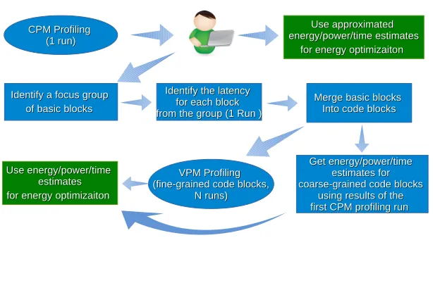
Fig. 6. The ALEA profiling process
mates. The offline module usesobjdump to disassemble the profiled program, and its own parsers to identify basic blocks and instructions inside these blocks. It uses this information to assign samples to specific blocks. Thus, ALEA can estimate the exe-cution time for each basic block, using the probabilistic model described earlier. To enable accurate energy and power profiling, the user should identify basic blocks to be merged into coarse-grained blocks if the default power model (CPM) is used. VPM can be applied to fine-grained blocks (with latency as low as 10µs, see Section 5.3), how-ever the user should point ALEA to these blocks. The user obtains the latency of each basic block by using an additional run and dynamic instrumentation tools, or direct instrumentation. Finally, we use DWARF debugging information to associate ALEA’s estimates with specific lines in the source code.
Figure 6 illustrates the process of profiling from the user perspective. During the first run of ALEA, the user identifies execution time, energy and power estimates for each basic block using CPM. From this point the user can do additional runs and select basic blocks where more accurate estimates are needed. This step can also be automat-ed with hotspot analysis, using, for example, clustering and classification techniques similar to the ones used in architectural simulators [Sherwood et al. 2001]. The us-er should point ALEA which basic blocks should be mus-erged into code blocks using addresses of these blocks. If latency of a merged code block is greater than the power-sensing interval then the results of the first profiling run could be used to get accurate power and energy estimates for this code block. If the latency of the code block is less than the power-sensing interval and no lower than 10 µs, then the user needs to run VPM for the specific code block and pass to ALEA the addresses of the first and last instructions and the latency of the block. The user can initiate any desirable number of profiling runs using CPM or VPM to achieve the desirable accuracy.
[image:10.612.156.463.106.307.2]4.1. Platforms and Energy Measurement
ALEA builds on platform-specific capabilities to measure power. It can use direct power instrumentation, integrated power sensors, or software-defined power models. ALEA operates under the sampling rate constraints of the underlying sensors, but is not limited by them since its probabilistic models can estimate power at finer code block granularity. To demonstrate the independence of our approach from the specifics of the hardware, we use two platforms that differ in architectural characteristics and support for power instrumentation.
Our first platform, a Xeon Sandy Bridge server, uses RAPL for on-chip software-defined modeling of energy consumption, which we obtain by accessing the RAPL M-SRs [Rotem et al. 2012]. The server includes 4 Intel Xeon E7-4860 v2 processors, each with 12 physical cores (24 logical cores) per processor, 32 KB I and D caches per core, a 3 MB shared L2 cache, and a 30 MB shared L3 cache per package. The system runs CentOS 6.5 and has a maximum frequency of 2.6 GHz.
Our second platform, an ODROID-XU+E board [Hardkernel 2016], has a single Exynos 5 Octa processor based on the ARM Big.LITTLE architecture, with four Cortex-A15 cores and four Cortex-A7 cores. In our experiments we only use the Cortex-Cortex-A15 cores at their maximum frequency of 1.6 GHz. Each core has 32 KB I and D-caches, while the big cores also share a 2 MB L2 cache. We measure power through the board’s integrated sensors. The system runs Ubuntu 14.04 LTS.
4.2. Power-Sensing Interval
Our Intel Sandy Bridge server provides energy estimates through RAPL, but not power measurements. We measure processor power consumption on it by dividing energy measurements taken at the start and end of the power-sensing interval by the size of this interval. The energy counter is updated only once per millisecond, which is the server’s minimum feasible power-sensing interval. Our Exynos platform includes the TI INA231 power meters [TI 2013], which directly sample power consumption for the whole system-on-chip and several of its components. These samples are averaged over a user-defined interval. The minimum available interval on the Exynos is 280µs.
Shorter power-sensing intervals improve CPM estimates for the fine-grained blocks. Thus, our CPM experiments use the minimum power-sensing interval on both plat-forms.
VPM assumes that we can precisely control when power is measured. Unfortunately, on Intel processors, RAPL energy counters are updated by the hardware at unknown points and transparently to software, with an update frequency of one ms. Thus, we cannot use VPM for Intel processors with RAPL. On the Exynos platform, even though we initiate the power measurement, a small variable delay occurs between the system call to read the power counters and the actual reading. Still, we can assume that this delay remains fixed on average and converges to its mean value as the number of samples increases.
0 10 20 30 40 50 60 70 80 90 Threads
0 5 10 15 20
Overhead per sample, msec
0.48
Sandy Bridge Run on a dedicated core Run on a shared core
1 2 3 4
Threads 0
2 4 6 8 10 12
Overhead per sample, msec 0.65
Exynos
Fig. 7. Overhead per sample versus number of threads with ALEA running on a dedicated or a shared core.
4.3. Sampling Interval and Overhead
The attach, deliver, and detach phases of the tool introduce overhead. The attach phase interrupts the execution of all threads. Threads continue to execute after completion of the detach phase.
We use a set of benchmarks from the NAS suite (BT,CG,ISandMG) to illustrate the profiling overhead of the ALEA online module, with a core dedicated to each applica-tion thread. We choose benchmarks that scale well so we can evaluate the overhead of ALEA under a difficult scenario in which the application utilizes the processor re-sources fully and is sensitive to sharing them with ALEA.
Figure 7 shows the overhead of ALEA, which clearly depends on the number of ap-plication threads, since the tool has to deliver the instruction pointer for each thread. With more threads the delivery overhead necessarily increases. The profiler can share a core with the program or it can use a dedicated core. We observe higher overhead when the tool and the program share a core, which is caused by a delay in the de-livery phase. This delay grows significantly, up to 10×, when the tool attaches to the application thread on the shared core due to the overhead of switching between an ap-plication thread and the ALEA profiler. The profiler leverages the OS load-balancing mechanisms to exploit idle cores, if available. The benchmarks occasionally leave cores idle and this slack grows as the benchmark uses more threads. Linux dynamically migrates profiled threads from a core used by ALEA to an idle one to eliminate the context-switching overhead, which leads to an overhead reduction as the number of threads grows on the Sandy Bridge platform when ALEA uses a shared core. Still, if the benchmarks use more than 30 threads the context-switching overhead becomes negligible in comparison to the overhead caused by the attach, deliver, and detach phases.
[image:12.612.133.480.97.201.2]R.heartwall
R.lud R.sc
R.srad
NAS.MGNAS.BTNAS.IS
NAS.CGR.cfd
R.kmeans
Runs
0
50
100
150
200
Error,%
0
10
20
30
40
50
Average error 1 run: 32.92%
Average error 180 runs: 2.11%
Peak
∞5
10
15
20
25
30
35
40
45
Fig. 8. Average error of energy estimates across all loops on Sandy Bridge
5. VALIDATION
In this section we validate the accuracy of our approach under extreme scenarios, where the power consumption changes rapidly and widely. We use multiple bench-marks on both hardware platforms to establish the generality of our results. We val-idate ALEA using loops with coarse-grained blocks for each platform. We then show that CPM (Section 5.1) can accurately estimate the energy consumption of coarse-grained blocks, while VPM (Section 5.2) does so even for fine-coarse-grained blocks.
5.1. Constant Power Model Validation
To validate the accuracy of ALEA’s energy consumption estimates, we use ten parallel benchmarks from the NAS and Rodinia suites. We use a wide range of benchmarks to achieve good coverage of loop features in terms of execution time and energy con-sumption, including loops with distinct power profiles and power variation between their samples. For each benchmark we compare CPM time and energy estimates for each loop with direct measurements. These direct measurements use instrumentation at the entry and exit points of the loops. On the Sandy Bridge platform we instrumen-t instrumen-the code using instrumen-the rdtsc instruction and the RAPL interface for time and energy
respectively. On Exynos we use clock gettime() to measure time and the ioctl()
interfaces to access the INA231 power sensors.
We compile the Rodinia benchmarks using the flags specified by the benchmark suite and run them with the default inputs. The benchmarks from NAS are built
using option CLASS=B and run with the default options. We use the abbreviation
suite.benchmark to indicate the benchmarks on our graphs. For example,R.sc cor-responds to the StreamCluster (SC) benchmark from the Rodinia suite.
5.1.1. Sandy Bridge.We run each benchmark using 96 threads on the Sandy Bridge
[image:13.612.166.512.85.312.2]R.heartwall
R.lud R.sc
R.srad
NAS.MGNAS.BTNAS.IS
NAS.CGR.cfd
R.kmeans
Runs
0
10
20
30
40
50
Error,%
0
5
10
15
20
Average error 1 run: 21.62%
Average error 50 runs: 1.03%
Peak 114.23%
2.5
5.0
7.5
10.0
12.5
15.0
17.5
20.0
22.5
Fig. 9. Average error of energy estimates across all loops on Exynos
We combine samples from multiple runs for each benchmark to achieve accurate estimates. We collected 500 runs for each benchmark but found the accuracy with 180 to be sufficient. Using more runs has little effect, so our remaining experiments use 180 runs.
Figure 8 shows how the error of energy estimates changes with the number of com-bined runs. IgnoringStreamCluster, the mean error is as high as 32% when we profile each benchmark only once. Predicting energy for StreamCluster requires more than one run. The total execution time of one instrumented loop is shorter than the sam-pling interval, so the loop may not be sampled during a run.
Increasing the number of combined runs reduces the error. On average, the error decreases to 2.1% after 180 profiling runs. Even for StreamClusterthe error is only slightly above average at 2.3%. Regarding the estimation of the total energy consump-tion of the program, the average error across all benchmarks is 1.6% for 180 runs. The energy estimates errors of ALEA are thus comparable to ALEA’s runtime overhead. For completeness, we also profile a 94-thread version of each benchmark with ALEA using a dedicated core. We used a sampling interval of 3 seconds to keep overhead low (under 1%). The minimum error of 1.9% with 155 runs is again comparable to the runtime overhead.
5.1.2. Exynos.We similarly validate ALEA on the Exynos platform. We used the same
experimental setup, except that we use two threads for the benchmarks to give ALEA a dedicated core and set the sampling interval to 500 ms with the aim of keeping the overhead slightly below 1%. Figure 9 presents the trade-off between the number of runs and the average error in our energy estimates for the loops. The sampling interval is longer than the average latency of almost all instrumented loops. The average error of the energy estimates is about 21% for a single profiling run but decreases to 1% with 50 or more profiling runs. The whole program absolute error for energy, averaged across all benchmarks, is 1.1% for 50 profiling runs.
[image:14.612.121.439.97.298.2]1 2 4 8 Power sensing interval,ms 0
10 20 30 40 50 60 70 80
Number of samples
loop with nops
1.0 7.5 13.0
Error of the power estimates provided by VPM
1 2 4 8
Power-sensing interval,ms 0
10 20 30 40 50 60 70 80
Number of samples
loop with cache accesses
3.5 7.0
[image:15.612.156.454.99.198.2]Error of the power estimates provided by VPM
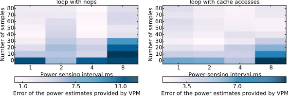
Fig. 10. Power estimates provided by VPM for the microbenchmark
run and the error in terms of both execution time and energy exceeded 120%. How-ever, this error falls below 5% within 50 runs. While ALEA can theoretically achieve any desirable accuracy, in practice the lower limit of the error is about 1% due to the instrumentation overhead and measurement interference.
We repeat our experiments using 4 threads for each benchmark, with ALEA shar-ing a core. The results show the same patterns, with the average error of the energy estimates at about 1.3% and stabilizing after 110 profiling runs.
5.2. Variation-Aware Power Model Validation
Next we validate the estimates produced by our Variation-Aware Power Model (VPM). These experiments only use the Exynos platform due to RAPL’s limitations (see Sec-tion 4.2). We design VPM to capture fine-grained program power behavior. Thus, we validate it on programs with significant power variation between fine-grained block-s: loops with latency less than the power-sensing interval. We use a 1100µs power-sensing interval for the reasons discussed in Section 4.2. On the other hand, to vali-date VPM we must use loops with known power consumption and latency. To measure them directly, latency must be above the minimum power-sensing interval (280µs).
5.2.1. Context-driven power variation.Our experiments show that processor
dynam-ic power consumption is primarily affected by cache and memory access intensi-ty [Mukhanov et al. 2015]. Thus, we use a microbenchmark that consists of two loops. The first loop contains a block withnopinstructions, consuming 1.68 Watts. The sec-ond loop contains a block with memory access instructions engineered to hit in the L1 cache, and consumes 2.54 Watts. We control the latency of each loop through the number of iterations. We set the latency of each loop close to 400µs, which is within the range of latencies discussed above.
We profile a 2-thread version of the microbenchmark 1000 times (ALEA runs on a dedicated core) to collect at least 80 samples, which ensures at least a 95% confi-dence interval of the power measurements within 1% of the mean. Figure 10 shows the trade-off between the number of samples and the average error of the power esti-mates provided by the VPM model, which we compare to direct power measurements. In this figure the darkness of the color indicates the average error of the power esti-mates. We change the power-sensing interval from 1 ms to 8 ms and use a one second sampling interval to keep overhead under 1%.
Even though VPM provides precise power estimates, interference from power mea-surements impacts its accuracy. While we expect the average error to be higher for a 4 ms interval than a 2 ms interval, our results show the opposite. We speculate that this happens because of OS interference, but performing kernel modifications to validate this hypothesis was beyond the scope of this paper.
We use the same experiment and 1000 runs to test CPM’s accuracy. Similarly to VPM, we vary the power-sensing interval from 1 ms to 8 ms. Regardless of the interval, the average error of CPM power estimates is 45.5% after 1000 runs (∼45.5% for the energy estimates), which is 12×higher than the average error of VPM. Clearly, VPM can successfully handle power variations across fine-grained blocks, which CPM and other known power measurement and modeling techniques can not.
5.2.2. Concurrency-driven power variation. We next investigate how CPM and VPM
han-dle power variations due to switching from executing parallel coarse-grained loops to executing sequential fine-grained loops. The sequential loops consume less pow-er since fewpow-er cores are active. The following benchmarks have sequential fine-grained loops that are surrounded by parallel coarse-fine-grained loops: Srad (Rodinia)
andStreamCluster (Rodinia). For those fine-grained loops, we artificially inflate their execution time, to allow direct measurements.
Similarly to the microbenchmark experiments, we run each benchmark 1000 times. We use 2 threads for each benchmark and run ALEA on a dedicated core. Similarly to the context-driven power variation experiment, we use a one second sampling interval to keep the overhead negligible. Our experiments show that the average error of VPM power estimates is 5.4% (∼5.5% for energy estimates), while the average error of CPM estimates is 15.7% (∼16% for energy estimates), almost 3×higher.
We repeat the experiments with 4 application threads (so ALEA must share a core) and a 1 ms power-sensing interval. Our results demonstrate that the average error of VPM power estimates is 6% (∼6% for energy estimates), while the average error of CPM estimates is 25% (∼25% for energy estimates). Again, VPM can handle programs with fast changing power behavior better than CPM and produces accurate estimates.
5.3. Limitations of ALEA
ALEA is a tool for fine-grained energy profiling. The probabilistic model of the tool makes it possible to estimate the execution time of a code block with high accura-cy even if the average execution time of the block is a few microseconds, while the sampling interval can be several seconds. However, our base power model (CPM) as-sumes that power remains constant during the power-sensing interval. VPM relaxes this assumption and captures power variation over intervals that are shorter than the power-sensing interval. Nonetheless, the resolution of this model is also limited.
100 101 102
Latency,µs
0.0 0.5 1.0 1.5
Power,W
Estimates for the loops
the 1-st loop(nops) the 2-nd loop(cache accesses) Measured power(the 1-st loop) Measured power(the 2-nd loop)
0 50 100 150 200 250 300Number of samples 8
6 4 2 0 2 4
Power,W
Estimates for the 1-st loop
latency 10 µs
latency 1 µs
Measured power
0 50 100 150 200 250 300Number of samples 2
1 0 1 2 3
Power,W
Estimates for the 2-nd loop
latency 10 µs
latency 1 µs
[image:17.612.128.482.97.184.2]Measured power
Fig. 11. Power estimates provided by VPM for the microbenchmark with reduced latencies of the loops
Figure 11 shows the results for the microbenchmark with loop latencies between 1 and 400µs. Dashed red lines correspond to the power consumption of each loop found in the experiments in Section 5.2.1. The leftmost plot depicts how the power estimates for the loops change with their latency. The middle plot shows how the power esti-mates for the loop with nops change with the number of samples, while the rightmost plot demonstrates the same for the loop with cache accesses. While we cannot directly validate the power consumption since the loop latencies are less than the minimum power-sensing interval (280µs), we expect that the difference in power consumption between these loops should remain constant for all loop latencies.
We observe the expected difference for latencies of at least 10µs (leftmost subplot of Figure 11). While ALEA can theoretically achieve any desirable accuracy, in practice the lower limit of the error is about 1% due to the instrumentation overhead and mea-surement interference. The error of the power estimates for 10µs is 6.9%. This latency is the maximum resolution of the power estimates provided by VPM. On the other t-wo subplots, we also observe that the power estimates for the loops with this latency clearly converge to the measured power as the number of samples grows. For latencies below 10µs, the estimates never converge due to the limited accuracy of the power sen-sors. To capture power variations over intervals with 1µs latency, the sensors should provide accuracy of measurements within10−4 Watts if a 1100µs power-sensing in-terval is used. Moreover, the time required to measure power varies over samples and this variation exceeds 1µs, which negatively impacts the power estimates.
ALEA could not reliably capture power variation between code blocks with execution times less than 10µs. Nonetheless, this interval is still 110 times shorter than the used power-sensing interval and 28 times shorter than the minimum feasible power-sensing interval in our platforms. As we show later, this resolution is sufficient to support energy optimization. To the best of our knowledge, ALEA is the first tool that provides accurate power estimates at this resolution.
6. DISCUSSION
6.1. Hysteresis in Power Measurements
The voltage regulator module adjusts the voltage level to mitigate these variations. However, it cannot always change voltage quickly enough. To maintain voltage at safe levels when the current increases significantly, the PDN uses decoupling capacitors close to the processor (or package or motherboard). On the Exynos board the power sensors (INA231) take power measurements on a power rail that connects the PMIC (Power Management Integrated Circuits,MAX77802), which provide a voltage regulator, with the chip. Decoupling capacitors, inductance and impedance components located between the power sensors and the die affect instantaneous power dissipation. Thus, the effect of a code block on the measured power is not instantaneous and hysteresis oc-curs between execution of the block and its effect on the measured power consumption. Moreover, capacitance components also smooth out instantaneous power dissipation.
ALEA’s probabilistic sampling can theoretically capture power shifts during instruc-tion execuinstruc-tion at any granularity. In practice, several factors, including software over-heads and the overover-heads and measurement error of the power sensing instruments, prevent such very fine granularity. The length of the hysteresis, i.e. the typical re-sponse time of the PDN, is orders of magnitude less than the minimum code block duration for which ALEA can probabilistically estimate power. The literature reports PDN response times in the range of 75 nanoseconds [Grochowski et al. 2002], versus
ALEA’s 10 µs minimum code block length and minimum power-sensing intervals on
the order of hundreds ofµs on the Exynos and Intel platforms.
6.2. Power modeling with performance counters
One of the possible solutions to break the coarse granularity of power sensors and miti-gate hysteresis effects is to predict power consumption from hardware activity vectors. Previous research has extensively investigated the use of regression models on activ-ity vectors of hardware performance counters to estimate power consumption. These models assume that processor power consumption correlates with the frequency of cer-tain performance impacting events. Performance counters can be accessed with low overhead on most modern processors, which makes them appropriate for fine-grained power modeling. We modify ALEA to use a regression model for power modeling fol-lowing Shen et al [Shen et al. 2013]. We use PAPI to measure non-halt core cycles, retired instructions per CPU cycle, floating point operations per cycle, last-level cache requests per cycle, and memory transactions per cycle over the power-sensing interval and then correlate these measurements to the sampled power consumption. We build the regression model for each platform individually on the basis of ten benchmarks used for validation of CPM and VPM with varying thread counts. We use a sampling interval that keeps runtime overhead under 1%. We add L1 cache accesses to the mod-el because its power consumption is highly sensitive to this event and omitting it loses significant accuracy.
In this experiment we use linear regression to predict power consumption for sam-ples that we use for training and compare the results of prediction with the power measurements taken for these samples. The average error of the power estimates pro-vided by the model is about 10% on both platforms, which is acceptable and consistent with the results demonstrated by Shen et al. However, the regression models produce anomalies by predicting the power of cache access intensive code blocks to be lower than the power of code blocks with nopinstructions. Thus, accuracy of the modeling could be insufficient to capture the effect of code blocks on power consumption, even though the average error of the linear regression is relatively small.
512Number of nodes1024 0 50 100 150 200 250 300 350 400 450 La te nc y, µ s 2.98x 4.54x
512Number of nodes1024 0 100 200 300 400 500 600 700 En er gy , 10 − 6J 2.87x 2.73x Optimized kernel Non-Optimized kernel
512Number of nodes1024 0.0 0.5 1.0 1.5 2.0 2.5 Power,W 1.7x
0 100 200 300 400Time
[image:19.612.114.500.98.195.2]10−5Sec 0.0 0.5 1.0 1.5 2.0 Power, W average power idle power kernel power
Fig. 12. Latency, energy and power for the binomial option pricing kernel. The rightmost plot presents power changes during run of the workload for the optimized kernel(512 nodes)
can be accessed by system software at once through the Performance Monitoring Unit (PMU). On the Exynos platform, the PMU module allows the user to sample only 7 performance counters at once. Thus, it is likely that RAPL achieves better accuracy by having fast hardware-supported access to many more performance counters than our model.
7. USE CASES
We now present practical examples of how ALEA enables energy-aware optimizations We first explore the effect of energy optimizations on power consumption in a latency-critical financial risk application where we apply VPM. We then demonstrate results for energy optimization based on runtime DVFS control using CPM.
7.1. Energy optimization of a latency-critical workload
We applied ALEA to profile and optimize a real-time and latency-critical option pric-ing workload. An option pricpric-ing model allows financial institutions to predict a future payoff using the current price and volatility of an underlying instrument. However, the current price is valid only for a limited interval, which implies that a decision about buying or selling the instrument is time critical. Binomial option pricing is a popu-lar pricing model that enables accurate prediction with low computational require-ments [Georgakoudis et al. 2016]. We use a commercial binomial option pricing kernel and a realistic setup that delivers requests to a worker thread running the kernel. The setup consists of two threads: the first thread listens to a TCP/IP socket, receives mes-sages and fills a queue with the mesmes-sages; the second thread parses the mesmes-sages and transfers requests to the worker thread. A third thread, the worker thread, processes option pricing requests.
The option pricing kernel uses the current price, volatility and number of nodes in the binomial tree as input parameters. The latency of the kernel depends only on the number of nodes since variation of the current price or volatility does not affect control and data flows of the kernel. Accuracy of the prediction is also primarily affected by the number of nodes in the binomial tree. While the current price and volatility could change in option pricing requests, in practice financial institutions use the minimal number of nodes which guarantees an acceptable quality of the prediction to reduce a pricing kernel response time. Consistent with this, the latency of the kernel should be a constant if the number of nodes does not vary. Following private communication with a leading financial institution, we used 512 nodes for realistic runs. The latency of the binomial option pricing kernel, which is about 177µs, is less than the power-sensing interval (280µs) for this number of nodes on the Exynos platform.
first code block builds a binomial tree and the second block computes the value of the option used to estimate the future payoff. To build the binomial tree, the first code block calls the exponential function in a loop, which is expensive in terms of energy and performance. The parameters of the function depend on an iteration of the loop and the underlying volatility, which is constant per request. To improve energy efficiency, we modified the kernel to dynamically identify the most frequently occurring volatility in option pricing requests and build at runtime an array containing the results of the exponent call for each iteration and this volatility (an example of memoization). In the optimized version of the kernel, we use the precomputed results instead of calls of the exponential function when the volatility of a request conforms with the most frequently occurring volatility.
Our experiments show that in 99.9 % of the samples, the first system thread executes the do futex waitsystem call and the second thread executes theepoll waitsystem call when the worker thread runs the kernel. Both system calls keep a core in sleep mode waiting for an incoming network message (the first thread) or a message from the queue (the second thread). The highest power consumption is observed when the worker thread runs the kernel.
We apply VPM to profile the kernel while reproducing a real workload of option pric-ing requests from an actual tradpric-ing day in the NYSE. Figure 12 shows latency, energy and power consumption of the optimized and non-optimized versions of the kernel. By applying memoization, we managed to reduce latency of the kernel by 2.98 times and energy consumption by 2.87 times with binomial trees of 1024 nodes. We also re-duced latency by 4.54 times for trees with 512 nodes. However, the energy reduction in this case was only 2.73 times. We explain this by a power spike that accompanied the latency reduction: the difference in the power consumption between the optimized and non-optimized versions for 512 nodes is 1.7 times, while this difference is only 4% for 1024 nodes. The explanation for the spike is that the number of cache accesses executed per second is higher in the optimized kernel with 512 nodes. These result-s demonresult-strate that energy and performance optimizationresult-s could lead to a result-significant rise in power consumption – which is a critical parameter for datacenter operators. ALEA provides the user with an option to choose an acceptable level of performance and energy optimization that meets a power budget. For example, on our Exynos plat-form, the user should not use the optimized version for binomial tress with 512 nodes and power capped at 2 Watt. As follows, ALEA enables users to optimize code under controlled power consumed at the fine-grained level without applying more intrusive power capping techniques such as DVFS [Petoumenos et al. 2015].
1 5 9 131721252933374145495357616569737781858993
Number of threads
2.6+ 2.5 2.4 2.3 2.2 2.1 2.0 1.9 1.8 1.7 1.6 1.5 1.4 1.3 1.2
Frequency , GHz
Min
Measurements:The NW benchmark
2.8 3.55 >4.3
Energy 103,J
1 5 9 131721252933374145495357616569737781858993
Number of threads
2.6+ 2.5 2.4 2.3 2.2 2.1 2.0 1.9 1.8 1.7 1.6 1.5 1.4 1.3 1.2
Frequency , GHz Min
Profiling:The computing block
1 1.75 >2.5
Energy 103,J
1
Number of threads
2.6+ 2.5 2.4 2.3 2.2 2.1 2.0 1.9 1.8 1.7 1.6 1.5 1.4 1.3 1.2
Frequency , GHz
Min
Profiling:The initialization block
1.61 1.8 >2
[image:21.612.111.504.94.209.2]Energy 103,J
Fig. 13. Energy consumption vs frequency and number of threads for the Needleman-Wunsch benchmark
7.2. Energy optimization with runtime DVFS control
The frequency that minimizes energy consumption depends on how intensely the cores interact with parts of the system not affected by frequency scaling, especially the main memory. Most existing approaches control frequency at the phase granularity, based on performance profiling, performance counter information, or direct energy measure-ments. We show how to use ALEA to drive decisions at any DVFS-supported granular-ity.
We use the Needleman-Wunsch benchmark from the Rodinia suite with a 40000×40000 matrix (∼6GB) as its input, executed on the Sandy Bridge platform. We first identify the optimal frequency and amount of parallelism for the whole pro-gram by taking energy measurements for the entire propro-gram. We test all combinations of frequency and number of threads. The leftmost plot of Figure 13 shows the result-s. The x-axis is the number of threads (1 to 96), the y-axis is frequency (1.2 to 2.6+ GHz), while the darkness of the color indicates energy consumption. The highest point on the y-axis, 2.6+ GHz, corresponds to enabled Intel Turbo Boost, in which case the processor can automatically raise the frequency above 2.6 GHz. The minimum energy consumption (2801 Joules) is observed when using 21 threads at 2.2 GHz.
ALEA finds two distinct code blocks that consume 99% of the total energy. The first code block uses one thread to initialize the arrays used by the benchmark. The second code block processes these arrays in parallel. We profile these blocks using CPM at different frequencies and with different thread counts for the second block. The middle and the rightmost plots of Figure 13 show the profiling results for the second and first blocks respectively. The two blocks consume their minimum energy at different frequencies, 2.5 GHz for the initialization block and 1.2 GHz for the computing block.
The blocks have different memory access patterns, which explains their energy pro-files. Both read data from an array much larger than the caches with similar frequency. However, the initialization block has high temporal and spatial locality so most memo-ry loads are serviced by the caches, processor stalls are few, and performance depends only on frequency. Thus, limiting the frequency too much increases execution time more than power reduction compensates. Alternatively, the computing block reuses data once or not at all, reading data from completely different pages in each iteration. Most accesses result in cache andTLBmisses, stalling the processor and making it run effectively at the speed of main memory. Lowering the frequency of the processor has little effect on performance, so the optimal choice is to use the lowest frequency.
of peak power, which is reached when executing the parallel computing group, the improvement is significant, 41.6%, while performance degradation is only 3.5%.
Several works consider different approaches to reduce energy consumption through runtime DVFS [Wu et al. 2005]. However, most of these works use analytical mod-els to predict the voltage and frequency setting which reduces energy consumption without a significant performance degradation. Central to such approaches is that the analytical models typically rely on parameters which have to be discovered for each platform individually. Moreover, the identified parameters do not guarantee the optimal voltage/frequency in terms of energy consumption. ALEA mitigates these re-strictions by assigning accurate power and energy estimates to source code for each voltage/frequency set.
8. RELATED WORK
PowerScope [Flinn and Satyanarayanan 1999], an early energy profiling mechanism, profiles mobile systems through sampling of the system activity and power consump-tion, which it attributes to processes and procedures.
The tool does not use a probabilistic model and does not address randomness of the sampling process to enable fine-grained energy profiling. PowerScope assumes that for most samples the program executes only one procedure during the sampling interval. This assumption holds only for coarse-grained procedures with latency greater than the sampling interval, which is approximately 1.6 ms in PowerScope. Therefore, the tool cannot perform energy accounting at a fine-grained level. Furthermore, the accu-racy of energy estimates is limited by the minimum feasible power-sensing interval provided by hardware sensors. In this paper we demonstrate that ALEA effectively mitigates all these restrictions by following a probabilistic approach.
Several tools for energy profiling use manual instrumentation to collect samples of hardware event rates from hardware performance monitors (HPMs) [Curtis-Maury et al. 2008; Bertran et al. 2013; Isci and Martonosi 2003; Li et al. 2013; Contreras and Martonosi 2005; Schubert et al. 2012]. These tools empirically model power con-sumption as a function of activity rates. These rates attempt to capture the utilization and dynamic power consumption of specific hardware components. HPM-based tools and their models have guided several power-aware optimization methods in comput-ing systems. However, they often estimate power with low accuracy. Further, they rely on architecture-specific training and calibration.
Eprof [Pathak et al. 2012] models hardware components as finite state machines with discrete power states and emulates their transitions to attribute energy use to system call executions. JouleUnit [Wilke et al. 2013] correlates workload profiles with external power measurement to derive energy profiles across method calls. JouleMe-ter [Kansal and Zhao 2008] uses post-execution event tracing to map measured energy consumption to threads or processes. While useful, these tools can only perform energy accounting of coarse-grained functions or system calls, which severely limits the scope of power-aware optimizations that can be applied at compile time or run time.
compo-nent between code blocks, while its statistical approach overcomes the limitations of coarse and variable power sampling frequency in system components.
Other energy profiling tools build instruction-level power models bottom-up from gate-level or design-time models to provide power profiles to simulators and hardware prototyping environments [Tu et al. 2014; Tsoi and Luk 2011]. These inherently static models fail to capture the variability in instruction-level power consumption due to the context in which instructions execute. Similarly, using microbenchmarks [Shao and Brooks 2013] to estimate the energy per instruction (EPI) or per code blocks based on their instruction mix does not capture the impact of the execution context.
9. CONCLUSION
We presented and evaluated ALEA, a tool for fine-grained energy profiling based on a novel probabilistic approach. We introduced two probabilistic energy accounting mod-els that provide different levmod-els of accuracy for power and energy estimates, depending on the targeted code granularity. We demonstrated that ALEA achieves highly accu-rate energy estimates with worst-case errors under 2% for coarse-grained code blocks and 6% for fine-grained ones.
ALEA overcomes the fundamental limitation of the low sampling frequency of power sensors. Thus, ALEA is more accurate than existing energy profiling tools, when pro-filing programs with fast changing power behavior. ALEA opens up previously unex-ploited opportunities for power-aware optimization in computing systems. Its portable user space module does not require modifications to the application or the OS for de-ployment. Using ALEA, we profiled two realistic applications and evaluate the effect of optimizations enabled uniquely by ALEA on their energy and power. Overall, ALEA supports simpler, more targeted application optimization.
Acknowledgement
This research has been supported by the UK Engineering and Physical
Sciences Research Council (EPSRC) through grant agreements EP/L000055/1 (ALEA), EP/L004232/1 (ENPOWER), EP/M01567X/1 (SANDeRs), EP/M015823/1, EP/M015793/1 (DIVIDEND) and EP/K017594/1 (GEMSCLAIM) and by the European Commission under the Seventh Framework Programme, grant agreement FP7-610509 (NanoStreams) and FP7-323872 (SCORPIO). We are grateful to Jose R. Herrero (UP-C), Pavel Ilyin (Soft Machines) and the anonymous reviewers for their insightful com-ments and feedback.
REFERENCES
Ramon Bertran, Alper Buyuktosunoglu, Pradip Bose, Timothy J. Slegel, Gerard Salem, Sean Carey, Richard F. Rizzolo, and Thomas Strach. 2014. Voltage Noise in Multi-Core Processors: Empirical Char-acterization and Optimization Opportunities. InProceedings of the 47th Annual IEEE/ACM Interna-tional Symposium on Microarchitecture (MICRO-47). IEEE Computer Society, Washington, DC, USA, 368–380.DOI:http://dx.doi.org/10.1109/MICRO.2014.12
Ramon Bertran, Marc Gonzalez Tallada, Xavier Martorell, Nacho Navarro, and Eduard Ayguade. 2013. A Systematic Methodology to Generate Decomposable and Responsive Power Models for CMPs.IEEE Trans. Comput.62, 7 (July 2013), 1289–1302.
Niels Brouwers, Marco Zuniga, and Koen Langendoen. 2014. NEAT: A Novel Energy Analysis Toolkit for Free-Roaming Smartphones. InProceedings of the 12th ACM Conference on Embedded Network Sensor Systems (SenSys ’14). ACM, New York, NY, USA, 16–30.