Improving Spark Application Throughput Via Memory Aware Task Co location:A Mixture of Experts Approach

Improving Spark Application Throughput Via Memory

Aware Task Co-location: A Mixture of Experts Approach

Anonymous Author(s)

Abstract

Data analytic applications built upon big data processing frameworks such as Apache Spark are an important class of applications. Many of these applications are not latency-sensitive and thus can run as batch jobs in data centers. By running multiple applications on a computing host, task co-location can significantly improve the server utilization and system throughput. However, effective task co-location is a non-trivial task, as it requires an understanding of the computing resource requirement of the co-running applica-tions, in order to determine what tasks, and how many of them, can be co-located. State-of-the-art co-location schemes either require the user to supply the resource demands which are often far beyond what is needed; or use a one-size-fits-all function to estimate the requirement, which, unfortunately, is unlikely to capture the diverse behaviors of applications.

In this paper, we present a mixture-of-experts approach to model the memory behavior of Spark applications. We achieve this by learning, off-line, a range of specialized memory mod-els on a range of typical applications; we then determine at runtime which of the memory models, or experts, best describes the memory behavior of the target application. We show that by accurately estimating the resource level that is needed, a co-location scheme can effectively determine how many applications can be co-located on the same host to improve the system throughput, by taking into consideration the memory and CPU requirements of co-running application tasks. Our technique is applied to a set of representative data analytic applications built upon the Apache Spark frame-work. We evaluated our approach for system throughput and average normalized turnaround time on a multi-core clus-ter. Our approach achieves over 86.4% of the performance delivered using an ideal memory predictor. We obtain, on average, 8.75x improvement on system throughput and a 51% reduction on turnaround time over executing applica-tion tasks in isolaapplica-tion, which translates to a 1.31x and 1.75x improvement over a state-of-the-art co-location scheme for system throughput and turnaround time respectively.

CCS Concepts • Computing methodologies → Dis-tributed algorithms;

Keywords Resource Modeling, Memory Management, Apache Spark, Task Scheduling, Predictive Modeling

Permission to make digital or hard copies of all or part of this work for personal or classroom use is granted without fee provided that copies are not made or distributed for profit or commercial advantage and that copies bear this notice and the full citation on the first page. Copyrights for components of this work owned by others than ACM must be honored. Abstracting with credit is permitted. To copy otherwise, or republish, to post on servers or to redistribute to lists, requires prior specific permission and/or a fee. Request permissions from [email protected].

Middleware’17,

©2017 ACM. xxx-xxxx-xx-xxx/xx/xx. . .$xx.00

DOI:xx.xxx/xxx x

ACM Reference format:

Anonymous Author(s). 2017. Improving Spark Application Through-put Via Memory Aware Task Co-location: A Mixture of Experts

Approach. InProceedings of ACM/IFIP/USENIX Middleware, ,

(Middleware’17),14 pages.

DOI:xx.xxx/xxx x

1

Introduction

Big data applications built upon frameworks such as Hive [41], Hadoop [36] and Spark [49] are commonplace. Unlike inter-active jobs, many of the data analytic applications are not latency-sensitive. Therefore, they often run as batch jobs in a data center. However, how to effectively schedule such applications to improve the server utilization and the system throughput remains a challenge.

Specifically, if an application task is given the entirety of main memory on each host to which it is deployed, it is effectively preventing the host machine from being used for any other application until the current one has finished, even if the task does not use all of the memory. Because many data analytic tasks do not use 100% of the CPU during execution [2, 24] there is a significant portion of unused processing capacity. An alternate approach is to share the computing host between multiple application tasks (where each task does not use all of the memory), this could save time and energy by co-locating processes more effectively on fewer machines.

Effective task co-locations require knowledge of the appli-cation’s resource demand. For in-memory data processing frameworks like Apache Spark, RAM consumption is a major concern [27]. It is particularly important to understand the memory behavior of the application. If we co-locate too many applications or give too much data to a single task, such that their total memory consumption exceeds the physical memory of the host, we could cause memory paging onto the hard disk, or an “out-of-memory” error, slowing down the overall system. To achieve this we need a technique to predict the precise memory requirement of any given Spark application.

In this paper, we present a generic framework to model the memory behavior of Spark applications. As a departure from prior work that uses a fixed utility function to model the resource requirement, we use multiple linear and non-linear functions to model the memory requirements of various applications. We then build a machine learning classifier to select which function should be used for a given application and dataset at runtime. As the program implementation, workload and underlying hardware changes, different models will be dynamically selected at runtime. Such an approach

is known asmixture-of-experts[23]. The central idea is that

instead of using a single monolithic model, we use multiple

models (experts) where each expert is specialized for

mod-eling a subset of applications. Using this approach, each memory model is used only for the applications for which its predictions are effective. One of the advantages of our approach is that new functions can easily be added and are selected only when appropriate. This means that the system can evolve over time to target a wider range of applications, by simply inserting new functions. The result is a new way of using machine learning for system optimization, with a generalized framework for a diverse set of applications.

We evaluate our approach on a 40-node multi-core cluster using 44 Spark applications that cover a wide range of appli-cation domains. We show that the accurate memory-footprint prediction given by our approach enables the runtime sched-uler to make better use of spare computing resources to improve the overall system throughput via task co-location.

We use two distinct metrics to quantify our results:system

throughputandaverage normalized turnaround time, and com-pare our approach against a state-of-art resource and task scheduler [10]. Experimental results show that our approach is highly accurate in predicting the application’s memory requirement, with an average error of 5%. By better utilizing the memory resources of a host, our system achieves 8.75x improvement of system throughput and a 51% reduction in application turnaround time. This translates to a 1.31x and 1.78x improvement over the state-of-art respectively on throughput and turnaround time.

This paper makes the following contributions:

∙ We present a novel machine learning based approach to

automatically learn how to model the memory behavior of Spark applications (Section 3);

∙ Our work is the first to employ mixture-of-experts for

resource demand modeling. Our generic framework allows new models to be easily added to target a wider range of applications and performance metrics;

∙ We show how to combine this resource modeling

frame-work with runtime task co-location policies to improve system throughput for Spark applications (Section 4);

∙ Our system is immediately deployable on real systems

and does not require any modification to the application source code.

2

Background and Overview

2.1 Apache Spark

Apache Spark is a general-purpose cluster computing frame-work [49]. with APIs in Java, Scala and Python and libraries

for streaming, graph processing and machine learning [49]. It is one of the most active open source projects for big data processing, with over 2,000 contributors in 2016. Each Spark

application runs as an independent set ofexecutor processes,

each with dedicated memory space for executing parallel jobs within the application. The executors are coordinated by the

driver program running on acoordinating node. Input data of Spark applications is stored in a shared filesystem and

or-ganized asresilient distributed datasets (RDDs) – a collection

of objects that can be operated on in parallel. Each Spark executor allocates its own heap memory space for caching

RDDs. This work exploits the data parallel property of RDDs

to characterize (or fingerprint) the application’s memory behavior without wasting computing cycles.

2.2 Problem Scope

Our goal is to develop a framework to accurately predict the resource requirement of Spark applications for arbitrary inputs. In this work, we focus on the memory requirement as RAM resources are a major concern for in-memory data pro-cessing frameworks like Apache Spark [27]. To demonstrate the usefulness of our approach, we apply it to perform task co-location for batched, data-analytic Spark applications. We do not consider latency-sensitive applications, such as search, as their stringent response time targets often require isolated execution [30].

Our approach estimates the memory footprint of a Spark executor for a given input dataset. It then uses this infor-mation to determine if there are enough spare resources (i.e. memory and CPU) to co-locate tasks; if there is, it calculates how many tasks could be co-located and how much work should be given to each task. We exploit the fact that many big data applications do not spend all of their time at 100% CPU [24] (see also Section 6.6). This observation suggests that there are opportunities to co-locate Spark tasks without sig-nificantly increasing the CPU contention and slow down the performance of co-running applications (see also Section 6.7). Our approach is applied to a simple task co-location policy in this work, yet the resulted scheme outperforms the state-of-the-art task scheduling scheme. We want to stress that our framework can be used by other scheduling policies to provide an estimation of the application’s resource demand to support decision making.

Our current implementation is restricted to applications whose memory footprint is a function of their input size, this is a typical behavior for many data analytical applications. In this work, we do not explicitly model disk and network I/O contention, because prior research suggests that they have little impact on the performance of in-memory processing frameworks including Apache Spark [35]. Nonetheless, our framework is general and allows new models to be easily added to target different applications, or other performance and resource metrics in the future.

2.3 Overview of Our Approach

Our approach, depicted in Figure 1, iscompletely automated,

Improving Spark Application Throughput Via Memory Aware Task Co-location: A Mixture of Experts Approach Middleware’17, ,

App Feature

Extraction

Model Calibration

1 2 3 4

Offline Profiling Runs

Memory footprint

Training programs

Model Fitting

Feature Extraction

f

Memory function

Feature values

Task Scheduling Func.

Prediction

Figure 1. Overview of how our approach can be used for task scheduling. For an incoming application, our approach first extracts the features of the program. Based on the fea-ture values, it predicts which of the off-line learned memory functions best describes the memory behavior of the applica-tion. It then instantiates the function parameters by profiling the application on some small sets of the input data items. A runtime scheduler then utilizes the memory function to perform task co-location.

An expert selector decides which model should be invoked, based on the runtime information of the application. To use our resource modeling framework to perform task co-location, a task scheduler follows a number of steps described as follows.

For each “new” application that is ready to run, we predict

which of theoff-line learned experts,termed ‘memory

func-tion’ in this paper, best describes its memory behavior, i.e. how the memory footprint changes as the input size varies. The selection of the memory function is based on runtime information of the program, such as the number of L1 data and instruction cache misses. This information is collected by running the application on a small portion (around 100MB)

of the input data items1_.

We then calibrate the selected function to tailor its pa-rameters to the target program and input. We do so by first profiling the application with two small different-sized parts of the application input to instantiate two function parameters; we then use the measured memory footprints to instantiate the parameter values. The calibrated memory function is then used to determine how many unprocessed data items should be allocated to an executor under a given memory budget. During the profiling run, we also record the average CPU usage of the application. After determining which memory function to use and obtaining the CPU usage of the application, the runtime scheduler can spawn new executors to run on servers that have spare memory, and if the aggregate CPU load of co-running tasks will go over 100% (i.e. to avoid CPU contention).

Since runtime information collection and model calibra-tion are all performed on some unprocessed data items and contribute to the final output, no computing cycle is wasted on profiling. Furthermore, we will re-run an executor process in isolation if it fails because of an “out-of-memory” error, but this was not observed in our experiments.

The key to our approach is choosing the right memory func-tion and then using lightweight profiling to instantiate the function parameters. An alternative is to use extensive pro-filing runs at runtime to find a model to fit the application’s memory behavior. However, doing so will incur significant overhead and could outweigh the benefit (see Section 6.4).

1_{We choose this modest input size as an input of this size typically}

takes a short time to process, while at the same time, it is sufficiently large (i.e. this often results in a working set that is larger than the size of the L3 data cache in most of the high-end CPUs) to capture the cache behavior of the application.

App

_Extraction

Feature

_Exam.

Func.

1 2 3 4

Offline Profiling Runs

Memory footprint Training

programs

Model Fitting

Feature Extraction

f

Memory function

Feature values

Task

Scheduling

5

Func.

Prediction

Figure 2.The training process.

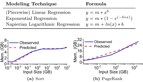
Table 1.Memory functions used in this work

Modeling Technique Formula

(Piecewise) Linear Regression 𝑦=𝑚*𝑥𝑏

Exponential Regression 𝑦=𝑚*(1−𝑒(−𝑏*𝑥)₎

Napierian Logarithmic Regression 𝑦=𝑚+𝑙𝑛(𝑥)*𝑏

1 0 - 3 _{1 0} - 2 _{1 0} - 1 _{1 0} 0 _{1 0} 1 _{1 0} 2 _{1 0} 3

0

2

4

6

8

M

em

. (

G

B)

I n p u t S i z e ( G B ) O b e s e r v e d P r e d i c t e d

(a)Sort

1 0 - 2 _{1 0} 0 _{1 0} 2

0

8

1 6 2 4 3 2

M

em

.

(G

B)

I n p u t S i z e ( G B ) O b e s e r v e d P r e d i c t e d

(b)PageRank

Figure 3.The observed and predicted memory footprints forSortandPageRankfrom HiBench. The memory footprint of the two applications can be accurately described using one of the memory functions listed in Table 1.

In the next section, we will describe how supervised ma-chine learning [1] can be used to construct the memory tions (experts) and the expert selector to choose which

func-tion to use for any “unseen” applications.

3

Predictive Modeling

Our approach involves using multiple memory functions (ex-perts) to capture the memory requirement of an application for a specific runtime input. The set of memory functions are constructed offline on a set of example programs, and then an expert selector dynamically chooses the best expert to use at runtime.

Our expert selector for determining the memory function

is a K-nearest neighbour (KNN) classifier [25]2. The input to

the classifier is a set of runtime features. Its output is a label to the memory function that describes the memory behavior of the target application and the specific dataset.

3.1 Learning Memory Functions

Our memory functions and expert selector are trained

off-lineusing a set of training benchmarks. The learned expert

selector can then be used to predict which memory function

to use for any new, unseen application. Figure 2 depicts

the process of collecting training data to learn the memory

functions to build theKNNclassifier. This involves finding a

mathematical function to model the memory footprint for each benchmark and collecting feature values of each training program.

2_{We have also explored several alternative classification techniques,}

During the training process, we run selected training pro-grams in isolation on a computing host. We profiled each training application with different sized inputs. For each pro-gram input, we record the memory footprint of the Spark executor process. Next, we try different mathematical mod-eling techniques to discover which model best describes the relationship between input size and memory allocation, that is, as the input size increases, how does the memory alloca-tion change. In this training phase, we record the memory function used to describe each training program. Our intu-ition is that the memory behavior for programs with similar characteristics will be similar. This hypothesis is confirmed in Section 6.8.

We use a set of linear and non-linear regression techniques to model the application’s memory behavior. Table 1 gives the full list of modeling techniques we used in this work. Each

of our models has two parameters,𝑚and𝑏, to be

instanti-ated during runtime model calibration. Here𝑥and𝑦are the

input size (i.e. the number ofRDDobjects in our case) and the

predicted memory footprint respectively. It is worth mention-ing that all the memory functions are automatically learned from training data, treating the applications as black boxes; new applications would similarly be learned automatically, potentially causing the addition of new memory functions.

Example.Figure 3 shows the observed memory footprint

and the prediction given by our memory function forSort

andPageRank. For these two applications, the memory func-tions used in this work can accurately model their memory

behaviors. Specifically, the memory footprint,𝑦, of Sortand

PageRankfor a given input size,𝑥, can be precisely described

using an exponential function ,𝑦=𝑚*(1−𝑒(−𝑏*𝑥)), where

𝑚= 5.768,𝑏= 4.479 and a Napierian logarithmic function,

𝑦=𝑚+𝑙𝑛(𝑥)*𝑏, where𝑚= 16.333,𝑏= 1.79 respectively. After building the memory functions, we need to have a mechanism to decide which of the functions to use. One of the key aspects in building a successful expert predictor is finding the right features to characterize the input application task. This process of feature selection is described in the next section. This is followed by sections describing training data generation and then how to use the expert selector at runtime.

3.2 Runtime Features

Raw Features.Expert selection is based on runtime char-acteristics of the application task. These charchar-acteristics,

calledfeatures, are collected using system-wide profiling tools:

vmstat, Linuxperfand performance counter toolPAPI. Col-lected feature values are encoded to a vector of real values. We considered 22 raw features in this work, which are given in Table 2. Some of these features are selected based on our intu-ition, while others are chosen based on prior work [11, 48]. All these features can be automatically and externally observed, without needing access to the source code.

Feature Scaling.Supervised learning typically works better if the feature values lie in a certain range. Therefore, we scaled the value for each of our features between the range of 0 and 1. We record the maximum and minimum value of each feature found at the training phase, and use these values

P C 5 3 % P C 4 4 % P C 3 7 % P C 2 1 0 %

P C 1 7 1 % R e s t P C s - 5 %

(a)Principal components

L1

_T

CM

L1

_D

CM

vc

ac

he

L1

_S

TM bo cs

0

5

1 0 1 5 2 0 2 5 3 0 3 5 4 0

%

o

f c

on

tri

. t

o

va

ria

nc

e

(b)Most important raw features

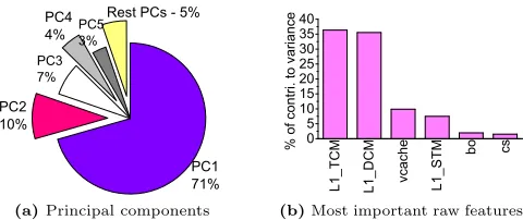
Figure 4.The percentage of principal components (PCs) to the overall feature variance (a), and contributions of the 5

most important raw features in thePCAspace (b).

to scale features extracted from a new application during runtime deployment.

Feature Reduction. Given the relatively small number of training applications, we need to find a compact set of features in order to build an effective predictor. Feature reduction is automatically performed through applying Principal

Compo-nent Analysis (PCA) on the scaled raw features. This technique

removes the redundant features by linearly aggregating

fea-tures that are highly correlated. After application ofPCA, we

use the top 5 principal components (PCs) which account for

95% of the variance of the original feature space. We record

thePCAtransformation matrix and use it to transform the

raw features of the target application toPCsduring runtime

deployment. Figure 4a illustrates how much feature variance that each component accounts for. This figure shows that prediction can accurately draw upon a subset of aggregated feature values.

Feature Analysis.To understand the usefulness of each raw

feature, we apply the Varimax rotation [32] to thePCAspace.

This technique quantifies the contribution of each feature to

eachPC. Figure 4b shows the top 5 dominant features based

on their contributions to the PCs. Cache features, L1 TCM,

L1 DCMandL1 STM, are found to be important for describing memory behaviors. This is not supervising as cache hit/miss rates are shown to be useful in characterizing the application behavior in prior works [6, 37]. Other features of virtual

memory usage (vcache), I/O (bo) and thread contention

(cs) are also considered to be useful, but are less important

compared to cache features. Using this technique, we sort the raw features listed in Table 2 according to the importance. The advantage of our feature selection process is that it automatically determines what features are useful when tar-geting a new computing environment where the importance of features may change.

3.3 Collect Training Data

We usecross-validation to construct memory functions and

theKNNclassifer to select which function to use. This standard

evaluation technique works by picking some target programs for testing and using the remaining ones for training.

Improving Spark Application Throughput Via Memory Aware Task Co-location: A Mixture of Experts Approach Middleware’17, ,

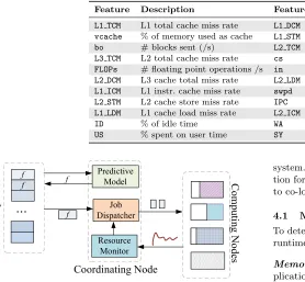
Table 2.Raw features, sorted by their importance

Feature Description Feature Description

L1 TCM L1 total cache miss rate L1 DCM L1 data cache miss rate

vcache % of memory used as cache L1 STM L1 cache store miss rate

bo # blocks sent (/s) L2 TCM L2 data cache miss rate

L3 TCM L2 total cache miss rate cs # context switches / s

FLOPs # floating point operations /s in # interrupts / s

L2 DCM L3 cache total miss rate L2 LDM L2 cache load miss rate

L1 ICM L1 instr. cache miss rate swpd % of virtual memory used

L2 STM L2 cache store miss rate IPC instruction per cycle

L1 LDM L1 cache load miss rate L2 ICM L2 instr. cache miss rate

ID % of idle time WA % of time on IO watting

US % spent on user time SY % spent on kernel time

E1

E2

E3

E4

E5

E6

T1

T2

T3

T4

T5

Time

Co

m

pu

tin

g

N

od

es

Ta

sk

Q

ue

ue

f

...

Co

m

pu

tin

g N

od

es

Predictive Model

Job Dispatcher f

Resource Monitor f

Coordinating Node f

Figure 5.Our system predicts the memory function for each application and monitors the memory resources of computing nodes. The runtime scheduler creates new executors to run on computing nodes that have spare memory, and uses the memory function to determine how much data should be given to the executor under a memory budget.

from the Spark-Perf [9] and the Spark-Bench [27] suites, although we did not directly train our models on them. The process of collecting training data is described in Figure 2. To collect training data, we first extract the feature values of each training program by running a single executor process in isolation, using inputs with an average size of 100MB. Next, we run each training program with different sized inputs

(ranging from∼300MB to∼1TB) and record the observed

memory footprints. We then find a memory function to closely fit the curve. For each training program, we store its principal component values and the memory function in a database.

Since training is only performed once, it is aone-off cost.

4

Runtime Deployment

Once we have learned the memory functions as described above, we can use a KNN algorithm to choose an appropriate

function to estimate the memory footprint for anyunseen

applications with a given input, and to use the prediction to co-locate Spark executor tasks at runtime.

Our runtime system built upon YARN [42], a task and resource manager for Spark. The co-location scheme will be triggered when more than one Spark application is waiting to be scheduled. Figure 5 illustrates the architecture of our

system. For each application task, we predict its memory func-tion for its input dataset, and then use the memory funcfunc-tion to co-locate Spark executor processes whenever possible.

4.1 Memory Requirement Prediction

To determine the memory function for an application task, a runtime system follows two steps, described as follows.

Memory Function Prediction.We run the incoming

ap-plication on a small set of the inputRDD objects (with an

aggregated size of around 100MB) to collect and

normal-ize feature values, and to perform thePCAtransformation.

We then calculate the Euclidean distance between the trans-formed input program feature vector and the feature vector

of each training program to find out thenearest neighbor,

i.e. the training program that is closest to the input pro-gram in the feature space (see also Section 6.8). We use the memory function of the nearest neighbor as the prediction. We also record the average CPU usage during this profiling run, and use this information later to determine whether co-location will cause CPU contention among co-running tasks. Our current implementation performs feature extraction by running the application on the lightly-loaded coordinating node (where the driver program runs). The results generated in the feature extraction phase will contribute to the final output of the application.

Model Calibration.After we have determined the memory function, we need to instantiate the function coefficients (i.e.

𝑚and𝑏in Table 1). We calculate these by running the

Furthermore, since the input and output data of the Spark application typically stored in a shared filesystem, we do not need to explicitly move the data in or out from the profiling host.

4.2 Resource Monitor

Each computing node runs a daemon that periodically reports to the resource monitor its memory usage and CPU load. Our current implementation reports the average memory usage and system load within a 5-minute window. The information

is retrieved from the Linux “/proc” system. Since this is

per-formed at a coarse-grained level (i.e. minutes), the overhead of monitoring and communication is negligible. With this monitoring scheme in place, a task scheduler can respond to execution phase changes and load variations, avoiding over-subscribing the computing resources.

4.3 Job Dispatcher

By default, we use the dynamic allocation scheme of Spark to determine how many free server nodes to use to run an application. However, the Spark dynamic scheme is not

perfect, so we utilize spare memory to spawn additional

executors to run on servers that have spare resources. Also, instead of waiting for the servers to become completely free, our approach starts executing waiting applications as soon as possible, reducing the turnaround time.

Once we have the memory function of the highest-priority application, the job dispatcher will spawn a new executor for the application to run on severs that have spare memory and if the aggregate CPU load of all co-running tasks will not go over 100%. The dispatcher uses the memory function to determine how much memory is needed for the remaining input (to allow us to co-locate more applications if possible), and how many data items can be cached by the executor un-der a given memory budget. To estimate the aggregate CPU load, we add up the CPU load of the computing host (which is reported by the resource monitor) and the average CPU usage of the application to be scheduled (which is obtained during the profiling run for feature collection). Furthermore, the number of data items to give to the co-located executor is dynamically adjusted over time, adapting to the changes of execution stages and memory resources. A naive alternative is to statically set the executor heap size to the size of free memory. But doing so can over-subscribe the memory re-sources than necessary and precludes co-locating more than two applications (see Section 6.1).

To minimize the potential thread contention, we dynami-cally adjust the number of threads (tasks) created by each executor to evenly distribute processor cores across currently-running executors on a single host. Furthermore, to enforce a certain degree of fairness, it is important to make sure that the new co-running task does not use the resources that are deemed to be essential for the currently running application. While fairness is not a focus of this work, our prediction framework helps the scheduler in this endeavor.

Table 3.Application task mixes used in the experiments

Label #App. Label #App. Label #App. Label #App.

L1 2 L2 6 L3 7 L4 9

L5 11 L6 13 L7 19 L8 23

L9 26 L10 30

5

Experimental Setup

5.1 Platform and Benchmarks

Hardware.We use a multi-core cluster with 40 nodes, each with an 8-core Xeon E5-2650 CPU @ 2.6GHz (16 threads with hyper-threading), 64GB of DDR4 RAM, and 16GB of swap. Nodes have SSD storage and are connected through 10Gbps Ethernet, precluding disk and network contention.

Software. Each computing node runs CentOS 7.2 with Linux kernel 3.12. We rely on the local OS to schedule processes and do not bind tasks to specific cores. We use Apache Spark 1.3.0 with Hadoop Yarn 2.4 as the cluster manager and HDFS as the Spark file management system. We use the Oracle Java runtime, Java SE 8u. We run Spark in the cluster mode. We also use the dynamic resource allocation scheme, so that memory will be given back to Spark when an application task completes. We run the Spark driver on a dedicated coordinating node and try to run multiple Spark executors on a single host to improve the system throughput. Finally, we use the Spark default configuration for memory management.

Workloads.We used 44 Java-based Spark applications from four widely used suites: HiBench [22], BigDataBench [16], Spark-Perf [9] and Spark-Bench [27]. These benchmarks im-plement the core algorithms used in real-life applications e.g. machine learning, image and natural language processing, and web analysis.

5.2 Evaluation Methodology

Runtime Scenarios.We evaluated our scheme using ten runtime scenarios with a mix of 2 to 30 randomly selected

ap-plications, detailed in Table 3. For each scenario, we try∼100

different application mixes and make sure all benchmarks are included in each scenario. The input size ranges from

small (∼300MB) and medium (∼30GB) to large (∼1TB).

In-puts were generated using the input generation tool provided by each benchmark suite. In the experiments, all tasks are scheduled on a first come first serve basis, but we stress that

our technique can be applied toany scheduling policy.

Predictive Model Evaluation.Our memory functions and predictor are trained using 16 benchmarks from HiBench and BigDataBench. We then apply the trained models to all 44 benchmarks from the four benchmark suites. When there are benchmarks from HiBench and BigDataBench present

in the task group, we use the standard

Improving Spark Application Throughput Via Memory Aware Task Co-location: A Mixture of Experts Approach Middleware’17, ,

suite from the training set. For example, when testingSort

from HiBench, we exclude Sort from BigDataBench from

training.

Performance Report. For each test case, we report the

performance asthe geometric meanacross all configurations.

We replay the schedule decisions for each test case multi-ple times, until the difference between the upper and lower confidence bounds under a 95% confidence interval setting is smaller than 5%. Furthermore, the time spent on feature extraction, model calibration, and prediction is included in our results.

5.3 Evaluation Metrics

We use two standard evaluation metrics for multi-programmed

workloads:system throughput andturnaround time. We use

the definitions given in [13], defined as follows.

1. System throughput (STP) is ahigher is better metric. It describes the aggregated progress of all jobs under co-location execution over running each job one by one using isolated execution. This is calculated as:

𝑆𝑇 𝑃= 𝑛

∑︁

𝑖=1 𝐶𝑖𝑖𝑠 𝐶𝑐𝑙 𝑖

(1)

wherenis the number of application tasks to be scheduled,

and𝐶𝑖𝑠𝑖 and𝐶

𝑐𝑙

𝑖 are the execution time for task𝑖under the

isolated execution mode (is) where the task uses all available

memory; and the co-locating mode (cl) where there may be

multiple tasks running on the same host.

2. Average normalized turnaround time (ANTT) is asmaller is bettermetric. It quantifies the time between a task being created and its completion, indicating the average user-perceived delay. This metric is defined as:

𝐴𝑁 𝑇 𝑇 = 1 𝑛

𝑛

∑︁

𝑖=1 𝐶𝑐𝑙

𝑖 𝐶𝑖𝑠

𝑖

(2)

5.4 Comparative Approaches

Quasar.This is a state-of-the-art co-location scheme [10].

Quasaruses classification techniques to determine the

char-acteristics of the application to perform resource allocation, and task assignment and co-location. Similar to our dynamic

scheme,Quasarmonitors workload performance to adjust

resource allocation and assignment when needed. Unlike our

approach,Quasaruses a single model for resource

estima-tion. To provide a fair comparison, we have implemented the

Quasarclassification scheme using the same set of training

programs that we used to build our models.

Pairwise.This pairwise co-location scheme looks for servers with spare memory to co-locate an additional task on the host. It sets the maximum heap size of the co-locating task to the size of free memory, and relies on the Spark default scheduler

to determine how many RDDdata items to be allocated to

the co-running task. This represents the default resource allocation policy used by many co-location schemes [29]. Oracle.We also compare our approach to the performance

of an ideal predictor (_Oracle) that gives the perfect memory

prediction for an application. This comparison indicates how

close our approach is to the theoretically perfect solution.

The prediction given by the Oracle scheme is obtained

through profiling the application on a given set of inputRDD

data items, but the profiling overhead is not included in the

results since we assume the_Oraclepredictor has the ability

to make prophetic prediction. Using theOraclepredictor,

the runtime scheduler can then search for the optimal number of data items to be given to a co-running task.

5.5 Highlights

The highlights of our evaluation are as follows:

∙ With the help of our mixture-of-experts approach, a

sim-ple task co-location scheme achieves, on average, a 8.75x improvement on STP and a 51% reduction on ANTT over isolated execution. This translates to a 1.31x and 1.75x improvement on STP and ANTT respectively, when

compared toQuasar. See Section 6.1;

∙ Our approach is highly accurate in predicting the memory

footprint of Spark applications, with an error of less than 5% for most cases. See Section 6.8;

∙ Our scheme is low-overhead. The time spent on feature

extraction and model calibration is less than 10% of the total application execution time, and the profiling runs contribute to the final results. See Section 6.5;

∙ We thoroughly evaluate our scheme by comparing it

against several alternative task co-location schemes and modeling techniques, and performing a detailed analysis on the working mechanism of the approach.

6

Experimental Results

In this section we first show the overall performance of our ap-proach against alternative schemes. We then provide analysis of the working mechanism of our approach.

Unless stated otherwise, we report each approach’s perfor-mance on STP and ANTT, by normalizing the results to a

baselinethat schedules the applications one by one with each application exclusively using all the memory of each allo-cated computing node. The normalized STP and ANTT are

referred to asnormalized STP andANTT reduction (shown

in percentage) respectively.

6.1 Overall Performance

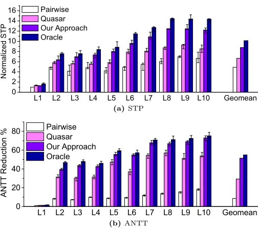
STP. Figure 6 (a) confirms that task co-location improves

system throughput. As the number of tasks to be scheduled

increases, we see an overall increase in the STP._Pairwise

performs reasonably well for small task groups, but it misses significant opportunities for large task groups. For L9 and

L10,Pairwiseonly delivers half of theOracleperformance.

This is because _Pairwise does not scale up beyond

pair-wise co-location.Quasarperforms significantly better than

Pairwiseby using a classifier model to coordinate resources

among co-locating tasks, but it is not as good as our ap-proach. By employing multiple functions to model diverse

applications, our approach constantly outperforms_Pairwise

andQuasaracross all task groups. For large task groups (L8

- L10), our approach delivers over 1.8x and 1.51x

improve-ment on the STP overPairwiseandQuasarrespectively.

L1 L2 L3 L4 L5 L6 L7 L8 L9 L10 Geomean 0

2 4 6 8 10 12 14 16

N

o

rm

a

liz

e

d

S

T

P

Pairwise Quasar Our Approach Oracle

(a)STP

L 1 L 2 L 3 L 4 L 5 L 6 L 7 L 8 L 9 L 1 0 G e o m e a n

0

2 0 4 0 6 0 8 0

AN

TT

R

ed

uc

tio

n

% P a i r w i s e _{Q u a s a r}

O u r A p p r o a c h O r a c l e

(b)ANTT

Figure 6.Our approach outperformsPairwiseandQuasar

on STP (a) and ANTT (b). The baseline is running the applications one by one using isolated execution. The min-max bars show the range of performance achieved across task mixes for each runtime scenario.

which translates to 65.7% of the_Oracleperformance. Our

approach achieves 8.75x improvement on STP, which

trans-lates to a 1.31x improvement overQuasaror 86.4% of the

Oracleperformance.

ANTT. Figure 6 (b) shows the ANTT reduction over the baseline. By maximizing the system throughput, task co-location in general leads to favorable ANTT results,

par-ticularly for large task groups.Quasar and our approach

outperformsPairwiseon ANTT by a factor of over 4x from

L2 onward. Our approach delivers better turnaround time

over Quasar, by avoiding memory contention among

co-locating Spark tasks. On average, our approach reduces the turnaround time by 51% across different task groups. This

translates to 94.6% of the_Oracleperformance. When

com-pared to the 54%Oracleperformance given by Quasar,

our approach achieves 1.75x better turnaround time.

Summary.We achieve 86.4% and 94.6% of the Oracle

performance for STP and ANTT respectively, outperforming

Pairwise, a widely used co-location policy, and Quasar,

a state-of-the-art co-location policy. The advantage of our approach is largely attributed to its use of multiple mod-els instead of just one to precisely capture an applications’ memory behavior. Without this accurate information, the alternative scheme often over- or under-provisions resources, leading to worse performance.

6.2 Server Utilization

Figure 7 shows the CPU utilization across 40 computing

nodes for_Pairwise,_Quasarand our approach when

sched-uling 30 Spark applications (L10), and Figure 8 presents the

0

5

1 0 1 5 2 0 2 5

ST

P P a i r w i s e Q u a s a r O u r a p p r o a c h

(a)STP (higher is better)

0

1 0 0 2 0 0 3 0 0

Tu

rn

ar

ou

nd

T

im

e

(m

in

)

P a i r w i s e Q u a s a r O u r a p p r o a c h

(b)Turnaround Time (lower is

bet-ter)

Figure 8.Resultant STP (a) and turnaround time (b) for the scheduling scenario in Figure 7. Our approach gives better STP and faster turnaround time when compared to alternative co-location schemes.

L 1 L 2 L 3 L 4 L 5 L 6 L 7 L 8 L 9 L 1 0 G e o m e a n

0

2

4

6

8

1 0 1 2 1 4

No

rm

al

ize

d

ST

P L i n e a r R e g r e s s i o n N a p i e r i a n L o g . R e g r e s s i o n E x p o n e n t i a l R e g r e s s i o n A N N O u r A p p r o a c h

(a)STP

L 1 L 2 L 3 L 4 L 5 L 6 L 7 L 8 L 9 L 1 0 G e o m e a n

0

1 0 2 0 3 0 4 0 5 0 6 0 7 0 8 0

AN

TT

R

ed

uc

tio

n

% L i n e a r R e g r e s s i o n N a p i e r i a n L o g . R e g r e s s i o n E x p o n e n t i a l R e g r e s s i o n A N N O u r A p p r o a c h

(b)ANTT

Figure 9.Compare to unified model based approaches that use a single modeling technique to describe the application’s memory behavior.

turnaround time (i.e. the wall clock time to finish the set of jobs) given by each approach. By carefully co-locating tasks using memory footprint predictions, our approach gives the best server utilization, which in turn leads to the highest STP

(1.84x and 1.43x higher STP over _Pairwiseand _Quasar

respectively) quickest turnaround time (1.5x and 1.32x faster

turnaround time over_Pairwiseand_Quasarrespectively).

6.3 Compare to Unified Models

Improving Spark Application Throughput Via Memory Aware Task Co-location: A Mixture of Experts Approach Middleware’17, ,

0 64 124 186 250 314 384

Time (min)

5 10 15 20 25 30 35 40

Nodes

0 20 40 60 80 100

Server Utilisation (%)

(a)Pairwise

0 64 124 186 250 314 384

Time (min)

5 10 15 20 25 30 35 40

Nodes

0 20 40 60 80 100

Server Utilisation (%)

(b)Quasar

0 64 124 186 250 314 384

Time (min)

5 10 15 20 25 30 35 40

Nodes

0 20 40 60 80 100

Server Utilisation (%)

(c)Our approach

Figure 7.CPU utilization across servers when scheduling 30 Spark applications (L10). The right-most non-zero point indicates the time when all applications finish. Our approach leads to the highest server utilization and quickest turnaround time.

L 1 L 2 L 3 L 4 L 5 L 6 L 7 L 8 L 9 L 1 0 G e o m e a n

0

2

4

6

8

1 0 1 2 1 4

No

rm

al

iz

ed

S

TP O n l i n e S e a r c h O u r A p p r o a c h

(a)STP

L 1 L 2 L 3 L 4 L 5 L 6 L 7 L 8 L 9 L 1 0 G e o m e a n

0

2 0 4 0 6 0 8 0 1 0 0

AN

TT

R

ed

uc

tio

n

% O n l i n e S e a r c h O u r A p p r o a c h

(b)ANTT

Figure 10. Compare to using online search to allocate in-put for a given memory budget. Our approach significantly outperforms the online search scheme, because it avoids the runtime overhead associated with finding the optimal number of data items to be given to the co-running task.

behaviors. Our approach outperforms ANN and all other approaches on STP and ANTT. The results suggest the need for using multiple modeling techniques to capture the di-verse application behaviors. This work develops a generic framework to support this.

6.4 Compare to Online Search

Figure 10 compares our approach to a method that uses descent gradient search to dynamically adjust the right input size for a given memory budget. The online search based approach gives rather disappointing results due to the large overhead involved in finding the right input size. Further-more, this approach also suffers from a scalability issue, i.e. the searching overhead grows as the number of computing nodes increases. Our approach avoids the overhead by di-rectly predicting the memory footprint, leading to 2.4x and 2.6x remarkably better performance on STP and ANTT respectively.

L 1 L 2 L 3 L 4 L 5 L 6 L 7 L 8 L 9 L 1 0

0

5 0 1 0 0 1 5 0 2 0 0 2 5 0 3 0 0

R

un

tim

e

(M

in

) M o d e l C a l i b r a t i o n _{F e a t u r e E x t r a c t i o n}

T o t a l E x e c u t i o n T i m e

Figure 11. Average profiling time to total task execution time. It is to note that during feature extraction and model calibration, the application always executes a portion of the unprocessed data, no computing cycles are wasted.

H B .S c a

n

B D B. G r e

p

H B .T e r a S or t

H B .J o i n

s

H B .A g g r e g at i o n B D B . W o

r d c ou n tH B .S o r

t

H B .W o r d c o_{B D B}u n t . S or t

H B .K m e a ns H B .P a g

e R an k B D B. C o

n . C_{H B .}o m .B a ye s B D B . N a

i v e B a y e

s

B D B . K m e a ns

B D B. P a g e R a n k

0

1 0 2 0 3 0 4 0 5 0

R

un

tim

e

(M

in

) M o d e l C a l i b r a t i o n _{F e a t u r e E x t r a c t i o n}

T o t a l E x e c u t i o n T i m e

Figure 12. Average profiling time to total runtime per program for HiBench and BigDataBench.

6.5 Profiling Overhead

0 - 1 0 1 0 - 2 0 2 0 - 3 0 3 0 - 4 0 4 0 - 5 0 5 0 - 6 0

0

2

4

6

8

1 0 1 2 1 4

#

Be

nc

hm

ar

ks

C P U L o a d i n I s o l a t i o n M o d e ( % )

Figure 13.CPU load distributions across benchmarks when the application is executed in the isolation mode.

6.6 CPU Load in Isolation Mode

Figure 13 shows the average CPU load when a benchmark is running in isolation using all the system’s memory exclusively. The CPU load for most of the 44 benchmarks is under 40%. As a result, the CPU is often not fully utilized when just running on application. This is in line with the finding reported by other researchers [2]. Our approach exploits this characteristic to improve the system throughput through task co-location. 6.7 Co-location Interferences

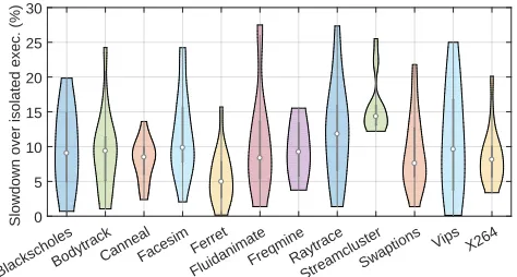
Interferences among Spark Benchmarks.The violin plot in Figure 14 shows the distribution of slowdown when running each of the 16 benchmarks from HiBench and BigDataBench along with each of the remaining 43 benchmarks using our scheme. The shape of the violin corresponds to the slowdown distribution. The thick black line shows where 50% of the data lies. The white dot is the position of the median. In the experiment, we first launch the target application and then use the spare memory to co-locate another competing

work-load. The input size of the target program is∼280GB. As

can be seen from the figure, the slowdown across applications is less than 25% and is less than 10% on average. For

ap-plications with little computation demand, such asHB.Sort,

the slowdown is minor (less than 5%). For benchmarks with

higher computation demand, such as HB.Aggregation, we

observe greater slowdown due to competing of computing resources among co-locating tasks. Overall, our co-location scheme has little impact on the application’s performance.

Interferences to PARSEC Applications.We further ex-tend our experiments to investigate the impact for co-locating Spark tasks with other computation-intensive applications. For this purpose, we run some computation-intensive C/C++ applications from the PARSEC benchmark suite (v3.0) [3] using the large, native input provided by the suite. Figure 15 shows the slowdown distribution of each PARSEC bench-mark when they run together with each of the 44 Spark benchmarks under our scheme. As all PARSEC benchmarks are share-memory programs, this experiment was conducted on a single host. As expected, we observe some slowdown to the computation-intensive PARSEC benchmark, but the slowdown is modest – less than 30%. For most of cases, the slowdown is less than 20%. Given the significant benefit on system throughput and server utilization given by our ap-proach, we argue that such a small slowdown is acceptable when maximizing the server utilization is desired (which is typical for many data center applications). There are other

HB.Sort

HB.WordCountHB.TeraSort HB.Scan

HB.Aggregation HB.Join HB.PageRankHB.Kmeans

HB.BayesBDB.Sort BDB.Wordcount

BDB.Grep

BDB.PageRankBDB.KmeansBDB.Con.Com BDB.NaivesBayes 0

5 10 15 20 25

Slowdown over isolated exec. (%)

Figure 14.Violin plot showing the distribution of slowdown when using our scheme to co-locate the target benchmark with another application on a single host. The baseline is running the target application in isolation. Here we run each of the 16 target benchmarks from HiBench and BigDataBench along with each of the remaining 43 benchmarks.

BlackscholesBodytrack

CannealFacesimFerret

FluidanimateFreqmineRaytraceStreamclusterSwaptions

Vips X264 0

5 10 15 20 25 30

Slowdown over isolated exec. (%)

Figure 15. The slowdown distribution of computation-intensive PARSEC benchmarks when they run with a Spark task under our scheme.

schemes such as Bubble-Flux [47] for reducing the interfer-ence via dynamically pausing non-critical tasks, which are orthogonal to our scheme.

6.8 Model Analysis

Program Distribution.Figure 16 visually depicts the dis-tribution of benchmarks on the feature space. To aid clarity,

we usePCAto project the dimension of the original feature

space down to two. Each point in the figure is one of the 44 benchmarks. This diagram clearly shows that the 44 bench-marks can be grouped into three clusters. After inspecting each cluster, we found that we indeed use the same mem-ory function (given on the figure) for all benchmarks in a cluster. This diagram justifies the chosen number of memory functions. It also confirms our assumption that programs with similar features can be modeled using similar memory functions. We want to highlight that one of the advantages

of ourKNNclassifier is that the distance used to choose the

Improving Spark Application Throughput Via Memory Aware Task Co-location: A Mixture of Experts Approach Middleware’17, ,

- 0 . 5 0 . 0 0 . 5 1 . 0 1 . 5 2 . 0 2 . 5

0 . 2 0 . 4 0 . 6 0 . 8 1 . 0 1 . 2 1 . 4 1 . 6

N a p i e r i a n L o g a r i t h m i c R e g r e s s i o n E x p o n e n t i a l R e g r e s s i o n

Pr

in

ci

pa

l C

om

po

ne

nt

2

P r i n c i p a l C o m p o n e n t 1 L i n e a r R e g r e s s i o n

Figure 16. Program feature space. The original feature

space is projected into 2 dimensions using PCA. Programs

can be grouped into three clusters. For all benchmarks in a cluster, their memory behaviors can be described using one of the three modeling techniques in Table 1.

- 5 . 7 %- 4 . 1 %- 2 . 7 %- 0 . 8 %- 4 . 8 %- 3 . 3 % 3 . 6 %- 2 . 6 % 1 . 4 %

1 2 % - 0 . 2 % 0 . 9 %

7 . 9 %_{- 0 . 1 %}- 1 . 6 % _{1 1 . 5 %}

H B .S c a

n

H B .A g g r e g at i o n B D B . W o

r d C o u n

t

H B .S o r

t

H B .J o i n

s

H B .W o r d C o u n

t

B D B . N a i v e sB a y

e s B D B. G r e

p

H B .T e ra S o r t B D B . S o

r t

B D B . C o n . C o m . B D B . K m

e a ns H B .P a g

e R a_{H B .}n kB a ye s H B .K m

e a ns

B D B . P a g e Ra n k

0

1 0 2 0 3 0 4 0

M

em

or

y

Fo

ot

pr

in

t (

G

B) P r e d i c t e d M e a s u r e d

Figure 17.Predicted memory footprints vs measured values for HiBench (HB) and BigDataBench (BDB).

how good the predicted memory function will be. If the target application is far from any of the clusters in the feature space, it suggests that a new memory modeling technique will be required (and our approach allows new memory functions to be easily inserted), or a conservative co-location policy should be used to avoid saturating the memory system.

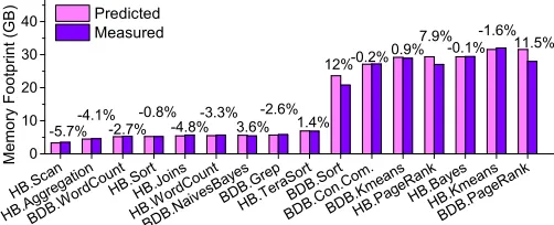
Prediction Accuracy.Figure 17 compares the predicted optimal memory allocation against the measured value, us-ing an input size of around 280GB. The prediction error of our approach is less than 5% in most cases except for HB.PageRank,BDB.PageRankandBDB.Sortfor which our ap-proach over-provisions around 8% to 12% of the memory. This translates to 1.5GB to 2GB of memory. Our approach also slightly under-estimates the memory requirement for some of the benchmarks, but the difference is small so it does not significantly affect the performance. In general, the accu-racy can be improved by using more training programs and more sophisticated modeling techniques to better capture the application memory requirement, which is our future work. In practical terms, one can also slightly over-provision (e.g. 10%) the memory allocation to applications with higher priorities to tolerate potential prediction errors. Overall, our approach can accurately predict the optimal memory allocation, with an average prediction error of 5%.

Table 4.Prediction accuracy for different classifiers

Classifier Accuracy (%) Classifier Accuracy (%)

Naive Bayes 92.5 SVM 95.4

MLP 94.1 Rand. Decision Forests 95.5

Decision Tree 96.8 ANN 96.9

KNN 97.4

Compare to Alternative Classifiers. Table 4 gives the memory function prediction accuracy (averaged across bench-marks and inputs) of various alternative classification

tech-niques and ourKNNmodel. The alternative models were built

using the same features and training data. Thanks to the high-quality features, all classifiers are highly accurate in

pre-dicting the memory function. We chooseKNNsimply because

it gives a similar prediction accuracy to alternative techniques but does not require re-training when a new memory function is added.

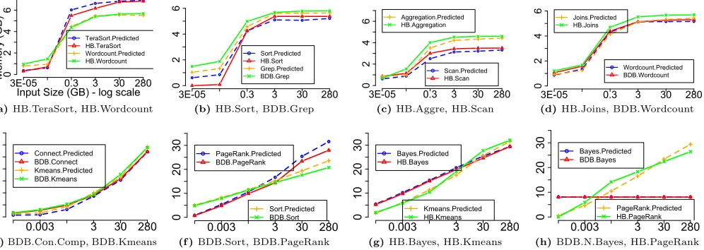
Memory Functions.Figure 18 compares the memory foot-print given by our approach to the measured values for Hi-Bench and BigDataHi-Bench, showing that our memory function can precisely capture the application’s memory footprint. This figure also shows that a single model is unlikely to capture diverse application behaviors. We address this by developing an extensible framework into which we can eas-ily plug-in multiple models to capture diverse application behaviors.

7

Related Work

Our work lies at the intersection between big data workload tuning and machine learning based system optimization.

7.1 Optimizing Big Data Workloads

Domain-specific Optimization.There exists a large body of work focusing on optimizing a single application using domain-specific knowledge. Prior work in domain-specific optimizations for single big data applications includes query optimization [4, 8, 45], graph or data flow optimization [5, 15, 26, 38], task tuning [7] and personal assistant and deep learn-ing services [20]. By contrast, we target resource modellearn-ing of Spark applications and demonstrate that this technique is useful for scheduling multiple application tasks.

Memory Management.Numerous techniques have been proposed to manage memory resources of big data applica-tions [40]. Many of the prior works require using dedicated

APIs to rewrite the application [14, 34]. Fang et al.

Input Size (GB) - log scale

Memory

(GB)

3E-050 0.3 3 30 280

2

4

6

TeraSort.Predicted HB.TeraSort Wordcount.Predicted HB.Wordcount

(a)HB.TeraSort, HB.Wordcount

3E-050 0.3 3 30 280

2

4

6

Sort.Predicted

HB.Sort

Grep.Predicted BDB.Grep

(b)HB.Sort, BDB.Grep

3E-050 0.3 3 30 280

2

4

6

Scan.Predicted HB.Scan Aggregation.Predicted

HB.Aggregation

(c)HB.Aggre, HB.Scan

3E-05 0.3 3 30 280

0

2

4

6

Wordcount.Predicted BDB.Wordcount Joins.Predicted

HB.Joins

(d)HB.Joins, BDB.Wordcount

0.003 3 30 280

0

10

20

30 _{Connect.Predicted}

BDB.Connect Kmeans.Predicted BDB.Kmeans

(e)BDB.Con.Comp, BDB.Kmeans

0.003 3 30 280

0

10

20

30 _{PageRank.Predicted}

BDB.PageRank

Sort.Predicted

BDB.Sort

(f )BDB.Sort, BDB.PageRank

0.003 3 30 280

0

10

20

30 _{Bayes.Predicted}

HB.Bayes

Kmeans.Predicted HB.Kmeans

(g)HB.Bayes, HB.Kmeans

0.003 3 30 280

0

10

20

30 _{Bayes.Predicted}

BDB.Bayes

PageRank.Predicted

HB.PageRank

(h)BDB.N.Bayes, HB.PageRank

Figure 18.Comparisons of the predicted memory footprint to the measured value.

Application Scheduling.Vermaet al. use profiling infor-mation to schedule jobs within a MapReduce application [43].

Mashayekhyet al.develop energy-aware heuristics to map

tasks of a big data application to servers to minimize energy usage [33]. Unlike our work, all these works target scheduling jobs within a single application, and allocate all physical memory of a machine to one single application. Other work looks at mapping parallelism by determining the number of cores and process time to be allocated to an application [19]. Our method promotes memory utilization on a local host, allowing the system to perform more tasks than previously allowed with current methods. Consequently, higher multi-tasking levels may lead to an increase in non-local data accesses within each task; the scheduling framework in [19] is therefore complementary to our work.

Task Co-location. Prior studies in task co-location include Bubble-Flux [47], Quasar [10], Tetris [17] and Cooper [29], which co-locate tasks across machines. Other studies sched-ule workloads on multi-core processors [28, 50]. All the ap-proaches mentioned above employ a single monolithic func-tion to model the resource requirement of applicafunc-tion tasks. There is little ability to examine whether the function fits the application under the current runtime scenario. Other fine-grained scheduling frameworks, like Mesos [21], rely on the user to provide the resource requirement of the applica-tion [21]. By contrast, we develop an extensive framework that uses multiple modeling techniques to automatically es-timate the resource requirement. Our approach allows new models to be added over time to target a wider range of appli-cations. Experimental results show that our approach yields better performance than a single model based approach. On the other hand, the co-location policies developed in these prior works for determining which two applications should co-locate are complementary to our work.

7.2 Predictive Modeling

Recent studies have shown that machine learning based pre-dictive modeling is effective in code optimization [39] and pro-cessor resource scheduling [44]. In [12], a mixture-of-experts approach is proposed to schedule OpenMP programs on multi-cores. Their approach uses multiple linear regression models to predict the optimal number of threads to use for a given program on a single machine. Our approach differs from [12] in two aspects. First, we target a different prob-lem (determining the memory footprint vs the number of threads) and a different scale (multiple vs a single node). Secondly, we use different modeling techniques, both linear and non-linear, to capture the memory behaviors of different applications. No work so far has used predictive modeling to model an application’s memory requirement to co-locate big data application tasks. This work is the first to do so.

8

Conclusions

This paper has presented a novel scheme based on a mixture-of-experts approach to estimate the memory footprint of a Spark applications for a given dataset. Our approach de-termines at runtime, which of the off-line learned functions should be used to model the application’s memory resource demand. One of the advantages of our approach is that it provides a mechanism to gracefully add additional expertise knowledge to target a wider range of applications.

We combine our resource prediction framework with a runtime task scheduler to co-locate latency-insensitive Spark applications. Using the accurate prediction given by our framework, a runtime task scheduler can efficiently dispatch multiple applications to run concurrently on a single host to improve the system’s throughput and at the same time to ensure the total memory consumption does not exceed the physical memory of the host. Our approach is applied to 44 representative big data applications built upon Apache Spark. On a 40-node cluster, our approach achieves, on

aver-age, 86% and 94.6% of theOracleperformance on system

Improving Spark Application Throughput Via Memory Aware Task Co-location: A Mixture of Experts Approach Middleware’17, ,

References

[1] Ethem Alpaydin. 2010. Introduction to Machine Learning(2nd

ed.). The MIT Press.

[2] Ahsan Javed Awan, Mats Brorsson, Vladimir Vlassov, and Eduard Ayguade. 2015. Performance characterization of in-memory data

analytics on a modern cloud server. InBig Data and Cloud

Com-puting (BDCloud), 2015 IEEE Fifth International Conference

on. IEEE, 1–8.

[3] Christian Bienia. 2011.Benchmarking Modern Multiprocessors.

Ph.D. Dissertation. Princeton University.

[4] Carsten Binnig, Norman May, and Tobias Mindnich. 2013. SQLScript: Efficiently analyzing big enterprise data in SAP

HANA. InLecture Notes in Informatics (LNI), Proceedings

- Series of the Gesellschaft fur Informatik (GI), Vol. P-214. 363–382.

[5] Vinayak Borkar, Michael Carey, Raman Grover, Nicola Onose,

and Rares Vernica. 2011. Hyracks: A flexible and extensible

foundation for data-intensive computing. InData Engineering

(ICDE), 2011 IEEE 27th International Conference on. IEEE, 1151–1162.

[6] John Cavazos, Grigori Fursin, Felix Agakov, Edwin Bonilla, Michael FP O’Boyle, and Olivier Temam. 2007. Rapidly selecting

good compiler optimizations using performance counters. In

Pro-ceedings of the International Symposium on Code Generation and Optimization. IEEE Computer Society, 185–197.

[7] Dazhao Cheng, Jia Rao, Yanfei Guo, and Xiaobo Zhou. 2014. Improving MapReduce Performance in Heterogeneous

Environ-ments with Adaptive Task Tuning. InProceedings of the 15th

International Middleware Conference (Middleware ’14). ACM, New York, NY, USA, 97–108.

[8] Tyson Condie, Neil Conway, Peter Alvaro, Joseph M. Hellerstein, Khaled Elmeleegy, and Russell Sears. 2010. MapReduce Online. InProceedings of the 7th USENIX Conference on Networked Systems Design and Implementation (NSDI’10). USENIX Asso-ciation, Berkeley, CA, USA, 21–21.

[9] Databricks. 2016. Spark-Perf. (2016). https://github.com/

databricks/spark-perf

[10] Christina Delimitrou and Christos Kozyrakis. 2014. Quasar:

Resource-efficient and QoS-aware Cluster Management. In

Pro-ceedings of the 19th International Conference on Architectural Support for Programming Languages and Operating Systems (ASPLOS ’14). ACM, New York, NY, USA, 127–144.

[11] Christophe Dubach, Timothy M. Jones, Edwin V. Bonilla,

Grig-ori Fursin, and Michael F. P. O’Boyle. 2009. Portable

Com-piler Optimisation Across Embedded Programs and

Microarchi-tectures Using Machine Learning. InProceedings of the 42Nd

Annual IEEE/ACM International Symposium on Microarchi-tecture (MICRO 42). ACM, New York, NY, USA, 78–88. [12] Murali Krishna Emani and Michael Boyle. 2015. Celebrating

Diversity: A Mixture of Experts Approach for Runtime Mapping

in Dynamic Environments. SIGPLAN Not. 50, 6 (jun 2015),

499–508.

[13] Stijn Eyerman and Lieven Eeckhout. 2010. Probabilistic Job

Symbiosis Modeling for SMT Processor Scheduling.SIGPLAN

Not.45, 3 (March 2010), 91–102.

[14] Lu Fang, Khanh Nguyen, Guoqing Xu, Brian Demsky, and Shan Lu. 2015. Interruptible Tasks: Treating Memory Pressure As

Inter-rupts for Highly Scalable Data-parallel Programs. InProceedings

of the 25th Symposium on Operating Systems Principles (SOSP

’15). ACM, New York, NY, USA, 394–409.

[15] Achille Fokoue, Oktie Hassanzadeh, Mohammad Sadoghi, and Ping Zhang. 2016. Predicting Drug-Drug Interactions Through

Similarity-Based Link Prediction Over Web Data. InProceedings

of the 25th International Conference Companion on World Wide Web (WWW ’16 Companion). International World Wide Web Conferences Steering Committee, Republic and Canton of Geneva, Switzerland, 175–178.

[16] Wanling Gao, Yuqing Zhu, Zhen Jia, Chunjie Luo, and Lei Wang. 2013. Bigdatabench: a big data benchmark suite from web search engines. 1–7.

[17] Robert Grandl, Ganesh Ananthanarayanan, Srikanth Kandula, Sriram Rao, and Aditya Akella. 2014. Multi-resource Packing for Cluster Schedulers, In Proceedings of the 2014 ACM Conference

on SIGCOMM.SIGCOMM Comput. Commun. Rev.44, 4 (Aug.

2014), 455–466.

[18] Dominik Grewe, Zheng Wang, and Michael FP OBoyle. 2013. OpenCL task partitioning in the presence of GPU contention. InInternational Workshop on Languages and Compilers for Parallel Computing. Springer, 87–101.

[19] Johann Hauswald, Yiping Kang, Michael A. Laurenzano, Quan Chen, Cheng Li, Trevor Mudge, Ronald G. Dreslinski, Jason Mars, and Lingjia Tang. 2015. DjiNN and Tonic: DNN As a Service and Its Implications for Future Warehouse Scale Computers, In

ISCA ’15.SIGARCH Comput. Archit. News43, 3 (June 2015),

27–40.

[20] Johann Hauswald, Michael A. Laurenzano, Yunqi Zhang, Cheng Li, Austin Rovinski, Arjun Khurana, Ronald G. Dreslinski, Trevor Mudge, Vinicius Petrucci, Lingjia Tang, and Jason Mars. 2015. Sirius: An Open End-to-End Voice and Vision Personal Assistant and Its Implications for Future Warehouse Scale Computers, In

ASPLOS ’15.SIGPLAN Not.50, 4 (March 2015), 223–238.

[21] Benjamin Hindman, Andy Konwinski, Matei Zaharia, Ali Ghodsi, Anthony D. Joseph, Randy Katz, Scott Shenker, and Ion Stoica. 2011. Mesos: A Platform for Fine-grained Resource Sharing in

the Data Center. InProceedings of the 8th USENIX Conference

on Networked Systems Design and Implementation (NSDI’11). 295–308.

[22] Shengsheng Huang, Jie Huang, Jinquan Dai, Tao Xie, and Bo Huang. 2011. The HiBench Benchmark Suite: Characterization

of the MapReduce-Based Data Analysis. InNew Frontiers in

Information and Software as Services: Service and Application Design Challenges in the Cloud, Divyakant Agrawal, K. Sel¸cuk Candan, and Wen-Syan Li (Eds.). Springer Berlin Heidelberg, Berlin, Heidelberg, 209–228.

[23] Robert A. Jacobs, Michael I. Jordan, Steven J. Nowlan, and Geoffrey E. Hinton. 1991. Adaptive Mixtures of Local Experts. Neural Comput.3, 1 (March 1991), 79–87.

[24] Tao Jiang, Qianlong Zhang, Rui Hou, Lin Chai, Sally A Mckee, Zhen Jia, and Ninghui Sun. 2014. Understanding the behavior of

in-memory computing workloads. InWorkload Characterization

(IISWC), 2014 IEEE International Symposium on Workload Characterization. IEEE, 22–30.

[25] James M. Keller and Michael R. Gray. 1985. A Fuzzy K-Nearest

Neighbor Algorithm.IEEE Transactions on Systems, Man and

Cybernetics(1985).

[26] Aapo Kyrola, Guy Blelloch, and Carlos Guestrin. 2012. GraphChi:

Large-scale Graph Computation on Just a PC. InProceedings

of the 10th USENIX Conference on Operating Systems Design and Implementation (OSDI’12). USENIX Association, Berkeley, CA, USA, 31–46.

[27] Min Li, Jian Tan, Yandong Wang, Li Zhang, and Valentina Sala-pura. 2015. SparkBench: A Comprehensive Benchmarking Suite

for in Memory Data Analytic Platform Spark. InProceedings of

the 12th ACM International Conference on Computing Fron-tiers (CF ’15). ACM, New York, NY, USA, Article 53, 8 pages. [28] Ming Liu and Tao Li. 2014. Optimizing Virtual Machine

Con-solidation Performance on NUMA Server Architecture for Cloud

Workloads.SIGARCH Comput. Archit. News42, 3 (jun 2014),

325–336.

[29] Qiuyun Llull, Songchun Fan, Seyed Majid Zahedi, and Benjamin C Lee. 2017. Cooper: Task Colocation with Cooperative Games. In High Performance Computer Architecture (HPCA), 2017 IEEE International Symposium on. IEEE, 421–432.

[30] David Lo, Liqun Cheng, Rama Govindaraju, Parthasarathy Ran-ganathan, and Christos Kozyrakis. 2015. Heracles: Improving

Resource Efficiency at Scale. InProceedings of the 42Nd Annual

International Symposium on Computer Architecture (ISCA ’15). ACM, New York, NY, USA, 450–462.

[31] Chi-Keung Luk, Sunpyo Hong, and Hyesoon Kim. 2009. Qilin: Ex-ploiting Parallelism on Heterogeneous Multiprocessors with

Adap-tive Mapping. InProceedings of the 42Nd Annual IEEE/ACM

International Symposium on Microarchitecture (MICRO 42). ACM, New York, NY, USA, 45–55.

[32] Bryan FJ Manly. 2004. Multivariate statistical methods: a

primer. CRC Press.

[33] Lena et al. Mashayekhy. 2015. Energy-Aware Scheduling of

MapReduce Jobs for Big Data Applications.IEEE TPDS(2015).

[34] Khanh Nguyen, Kai Wang, Yingyi Bu, Lu Fang, Jianfei Hu, and

Guoqing Xu. 2015. FACADE: A Compiler and Runtime for

(Almost) Object-Bounded Big Data Applications. InProceedings

of the Twentieth International Conference on Architectural Support for Programming Languages and Operating Systems (ASPLOS ’15). ACM, New York, NY, USA, 675–690.

[35] Kay Ousterhout, Ryan Rasti, Sylvia Ratnasamy, Scott Shenker, and Byung-Gon Chun. 2015. Making Sense of Performance in

Data Analytics Frameworks. InProceedings of the 12th USENIX