Munich Personal RePEc Archive
Fat-tailed uncertainty and the
learning-effect
Hwang, In Chang
14 February 2014
Online at
https://mpra.ub.uni-muenchen.de/53671/
Fat-tailed Uncertainty and the Learning-effect
In Chang Hwang
VU University Amsterdam, Institute for Environmental Studies, Amsterdam, The
Netherlands
De Boelelaan 1087, Amsterdam, The Netherlands, 1081 HV, E-mail: [email protected]
Abstract
One of the recent findings in the economics of climate change is that emissions control plays
a significant role in the reduction of the tail-effect of fat-tailed uncertainty on welfare. The
current paper gives another perspective: the learning-effect. The effect of emissions control
on welfare is decomposed into the direct effect and the learning-effect. Although this has
been known for thin-tailed uncertainty in the literature, this paper takes a different approach:
the changes in temperature distributions under fat-tailed uncertainty and learning.
Key words
Climate policy; deep uncertainty; Dismal Theorem; tail-effect; learning-effect
JEL Classification
1 Introduction
One of the recent findings in the economics of climate change is that optimal carbon tax does
not accelerate for many plausible situations as the uncertainty about climate change increases
(Karp, 2009; Hwang et al., 2013a, b; Millner, 2013; Horowitz and Lange, 2014), as implied
by Weitzman’s Dismal Theorem (Weitzman, 2009). This is because emissions control,
together with investment, which was absent in the model of Weitzman (2009), plays a
significant role in the reduction of the effect of fat-tailed uncertainty on welfare (the
tail-effect).
Beside its direct impact, emissions control has an implicit impact on welfare in that carbon
emissions produce information on the true state of the world through increased warming.
Since learning or the (partial) resolution of uncertainty has value, this should be accounted
for when the decision on emissions control is made.
The hypothesis of this paper is that the possibility of learning reduces the marginal benefits
of emissions control, compared to the case where there is no learning. As a result, learning
reduces the stringency of climate policy compared to the no-learning case. Although this has
been known for thin-tailed uncertainty in the literature (e.g., Kolstad, 1996a, b; Ulph and
Ulph, 1997; Kelly and Kolstad, 1999; Webster, 2002; Ingham et al., 2007), this paper takes a
different approach: the changes in temperature distributions under fat-tailed uncertainty. This
approach is also taken by Pindyck (2011, 2012) and Millner (2013), but their models are too
stylized and furthermore do not account for learning.
Section 2 presents the model. Sections 3 and 4 investigate the changes in temperature
distribution and the rate of tail-slimming (Weitzman, 2013), respectively. The main results
2 The Model
The learning-effect is discussed in this paper with a simple dynamic model as in Equation (1).
The problem of a decision maker is to choose the rate of emissions control in each period so
as to maximize social welfare defined as the discounted sum of expected utility of
consumption.
( ) ( ) ∫ (1)
where is social welfare, is time period, is the rate of emissions control, is the
utility function, is the discount factor, is the expectation operator, is consumption
per capita, is an uncertain parameter such as the equilibrium climate sensitivity,
is the set of any variable, and is the probability distribution function (PDF) of .
A unit increase in carbon emissions induces higher temperature in the future through
Equations (2-4).
( ) ( ) (2)
( ) (3)
( ) (4)
where is the carbon stock, is the emission-output ratio, is gross output per capita,
is the depreciation rate of the carbon stock, is radiative forcing from the carbon stock,
is radiative forcing from a doubling of carbon dioxide, is air temperature deviations
Equation (4) says that a doubling of carbon dioxide induces a temperature increase of ,
the equilibrium climate sensitivity. Without loss of generality it is assumed that ,
, and in this paper.
Carbon emissions reduce expected social welfare due to the loss of consumption as a
consequence of adverse climate change (Equation 5). Thus the decision maker tries to control
the amount of carbon emissions. Emissions control comes at a cost as in Equation (6).
⁄( ) (5)
(6)
where is the abatement cost function, (>0), (>0), (>1) and (>1) are economic
parameters. For simplicity is normalized to be one.
Equations (2-6) and the conditions for the parameter values are generally consistent with
the literature (e.g., Gregory and Forster, 2008; Nordhaus, 2008; Weitzman, 2012).
The hyperbolic absolute risk aversion (HARA) utility function is applied in this model.
Note that the constant relative risk aversion (CRRA) utility function, usually used in the
literature, is a special case of HARA. If (7) becomes CRRA.
( ) (7)
where , (≥0), and (>0)are parameters. It is assumed that ( ) ⁄ for utility to be
The uncertain parameter is assumed to have a fat-tailed distribution in the sense that
probability density diminishes slowly than exponentially in the upper tail (Weitzman, 2009;
Pindyck, 2011). In this paper the distribution of Roe and Baker (2007) is applied, which is
widely discussed in the literature (e.g., Weitzman, 2009; Millner, 2013). Applying the other
fat-tailed distributions does not affect the general findings of this paper, as argued in Hwang
et al. (2013). The notation for time is dropped for convenience, unless otherwise confused.
√ {
[( ̅ )] }
(8)
where ̅ and are the parameters of the climate sensitivity distribution, is a constant.
To solve the learning model, the random variable is transformed to derive the PDF of
temperature increases as follows.
( ) √
{ [
̅ ]
}
(9)
where is the PDF of future temperature increases and ( ) ( ) . Note that is
a fat-tailed distribution in that
⁄ ( ) for any .
3 Temperature Distribution and Tail-slimming Rate
The parameters and ̅ are subject to change in the learning model. For instance, the
belief of the decision maker on the climate sensitivity can be updated as information (e.g.,
literature, with a normal likelihood function, it is well known that the posterior mean tends to
the (pre-specified) true value and the posterior variance approaches zero asymptotically over
time (Cyert and DeGroot, 1974). With this in mind and without loss of generality, it is
assumed that ̅ ⁄ . The general findings of this paper are not affected by this
assumption. In addition, following the literature on learning (e.g., Kelly and Kolstad, 1999;
Leach, 2007) it is assumed that ⁄ . For instance, Hwang et al. (2014) find that
⁄( ⁄ ), where is the variance of temperature shocks and is a
parameter. Since ⁄ , it is clear that ⁄ ( ⁄ ) ( ⁄ ) . Together
with the fact that ⁄ from Equation (2-4), this translates into ⁄ ( ⁄ )
( ⁄ )
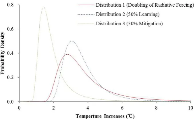
The PDFs of temperature increases for three hypothetical scenarios are illustrated in Figure
1. Distribution 1 refers to the case where radiative forcing is doubled relative to the
pre-industrial level. Distributions 2 and 3 refer to the cases where there is learning (a 50%
reduction in ) and there is a 50% reduction in carbon emissions, respectively compared to
the case for Distribution 1. Since this paper focuses on the tail-effect, only the probability
density of the upper tail is considered below. This is reasonable in that the upper tail
dominates the others in a usual cost-benefit analysis under deep uncertainty (Weitzman,
2009). As shown in the figure, for any in the upper tail, probability density increases in
radiative forcing ( ⁄ ). Likewise, for any in the upper tail, probability density
Figure 1 PDFs of temperature increases
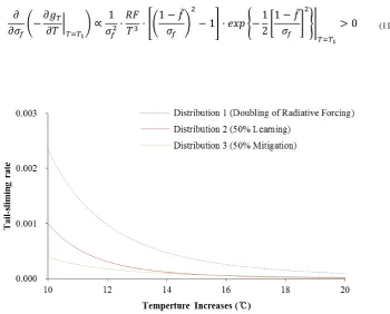
One of the important things to be considered in the economics of catastrophic climate
change is the rate of tail-slimming in the bad tail (Weitzman, 2013). If the tail-slimming rate
of the upper tail is slower than the one for objective function, willingness to pay to avoid
catastrophic climate change becomes arbitrarily large.
The tail-sliming rate at temperature in the upper tail can be defined as in Equation (10).
Since the fatness of the PDF decreases as temperature increases in the upper tail, the negative
sign is attached in Equation (10).
|
√
{ [
̅ ]
} {
( ̅ ) }||
→ √ { [ ̅]}|
As expected, the tail-sliming rate is increasing in radiative forcing (see also Figure 2). This
means that carbon emissions play a role in reducing the fatness of the upper tail, other things
being equal. In addition, the tail-sliming rate is increasing in uncertainty as in Equation (11).
This implies that learning is faster for larger uncertainty.
(
| )
[( ̅) ] { [ ̅] }|
[image:9.595.137.488.194.476.2]
(11)
Figure 2 Tail-sliming rate of each distribution in Figure 1
4 The Learning-effect
From Equation (1), optimal climate policy should satisfy the first order condition as follows.
For simplicity arguments of each function are dropped.
∫
( )
The left hand side (LHS) of Equation (12) is the marginal abatement costs, whereas the
right hand side (RHS) is the expected marginal benefits of emissions control (or the expected
marginal avoided damage costs).
Without loss of generality we consider a three-period problem below. For the last period it
is assumed that and ( ). The problem is recursively solved by backward
induction (Bellman and Dreyfus, 1962). If is assumed to be a solution for the second
period, given , the maximized social welfare is calculated as in Equation (13).1
( ) ∫ ( ) ( ̅ )
(13)
where ( | ), ( | ), ( | ), ̅ ̅ ( | ), ( | ).
The first order condition for the first period reads:
( )
( ) ∫ (
)
(14)
where ( ̅ ), ( ), ̅ ̅( ), ( ).
Substituting Equation (13) into Equation (14) and rearranging lead to Equation (15).
1 Hwang et al. (2013a) investigates the conditions for the convergence of RHS in Equation (12) under the
( ) ( ) ∫ ( ( ) ) ∫ { ∫ ( ( ) ) } (15)
Equation (15) says that the marginal benefits of emissions control are the discounted sum
of the expected marginal social welfare. The last term of RHS can be decomposed applying a
chain rule:
∫ ∫ { ( ) ( ) ( ) } ( )
(16)
The last term in the bracket of RHS can be further decomposed into Equation (17). Note
that it has been assumed that ̅⁄ .
(17)
The first term of RHS in Equation (17) reflects the effect of emissions control on the PDF
of temperature increases through the changes in radiative forcing, whereas the second term is
added because the parameters of the distribution change as learning takes place. Thus the
second term is named the ‘learning-effect’ hereafter.2
2
Note that the PDF of temperature increases for the second period changes only by radiative forcing.
The conditions for RHS in Equation (15) to converge do not change from the no-learning
case of Hwang et al. (2013), since the first term in RHS dominates the other terms regarding
the existence of solutions.
It is clear that ( ⁄ ) ( ⁄ ) and ( ⁄ ) ( ⁄ ) in the upper tail
from Figure 1. These relations imply that the learning-effect offsets to some extents the effect
of deep uncertainty on welfare. The marginal benefits of emissions control falls as the
decision maker learns, and thus the optimal level of emissions control or carbon tax decreases
when there is a possibility of learning, compared to the no-learning case.
The offsetting ratio is calculated as in Equation (18). The ratio grows in three conditions: 1)
the quality of information that carbon emissions produce ( ⁄ ) increases, 2) carbon
emissions are larger ( ), and 3) the level of learning is larger ( ⁄ ).
|( ⁄ ) ( ( ⁄ ) ⁄ )| ( ̅ ) ( ̅ ) →
(18)
Finally let us consider the case for active learning. Active learning refers to the case where
the decision maker explicitly affects the rate of learning (see Hwang et al., 2013c). If the
decision maker invests on climate science to raise the speed of learning (R > 0, where R is the
amount of investment), and if research is effective in reducing uncertainty ( ⁄ < 0), then
the offset ratio becomes far larger (see Equation 18). Consequently, there is an additional
reduction of the marginal benefits of emissions control, hence the less stringent climate
5 Conclusion
The effect of learning under fat-tailed uncertainty has been investigated in this paper using a
simple dynamic model. The effect of emissions control on welfare is decomposed into the
direct effect and the learning-effect. Main findings of this paper are that the possibility of
learning reduces the marginal benefits of emissions control, compared to the case where there
is no learning. As a result, learning reduces the stringency of climate policy. The fatter is the
tail of the distribution and the faster is learning the larger is the learning-effect. Hwang et al.
(2013c, 2014) investigate this issue with numerical models.
Acknowledgement
I am very grateful to Richard S. J. Tol and Marjan Hofkes for their helpful comments and
suggestions. The remaining errors are my own.
References
Bellman, R., Dreyfus, S.E., 1962. Applied dynamic programming. The RAND Corporations.
Cyert, R.M., DeGroot, M.H., 1974. Rational expectations and Bayesian analysis. The Journal
of Political Economy 82, 521-536.
Gregory, J.M., Foster, P.M., 2008. Transient climate response estimated from radiative
forcing and observed temperature change. Journal of Geophysical Research 113, D23105.
Horowitz, J., Lange, A., 2014. Cost-benefit analysis under uncertainty: A note on
Weitzman’s dismal theorem. Energy Economics 42, 201-203.
Hwang, I.C., Reynès, F., Tol, R.S.J., 2013a. Climate policy under fat-tailed risk: An
application of DICE. Environmental and Resource Economics 56(3), 415-436.
Hwang, I.C., Tol, R.S.J., Hofkes, M.W., 2013b. Tail effects and the role of emissions control.
Hwang, I.C., Tol, R.S.J., Hofkes, M.W., 2013c. Active learning about climate change.
University of Sussex Working Paper Series No. 65-2013.
Hwang, I.C., Tol, R.S.J., Hofkes, M.W., 2014. The effect of learning on climate policy under
fat-tailed uncertainty. Unpublished manuscript. The earlier version was presented at the 20th
EAERE Conference, June 2013, Toulouse, France.
Ingham, A., Ma, J., Ulph, A., 2007. Climate change, mitigation and adaptation with
uncertainty and learning. Energy Policy 35, 5354-5369.
Karp, L., 2009. Sacrifice, discounting and climate policy: five questions. CESifo Working
Paper No. 2761.
Kelly, D.L., Kolstad, C.D., 1999. Bayesian learning, growth, and pollution. Journal of
Economic Dynamics and Control 23, 491-518.
Kolstad, C.D., 1996a. Learning and stock effects in environmental regulation: the case of
greenhouse gas emissions. Journal of Environmental Economics and Management 31, 1-18.
Kolstad, C.D., 1996b. Fundamental irreversibilities in stock externalities. Journal of Public
Economics 60, 221-233.
Leach, A.J., 2007. The climate change learning curve. Journal of Economic Dynamics and
Control 31, 1728-1752.
Millner, A., 2013. On welfare frameworks and catastrophic climate risks. Journal of
Environmental Economics and Management 65, 310-325.
Nordhaus, W.D., 2008. A question of balance: Weighing the options on global warming
policies. New Haven and London: Yale University Press.
Pindyck, R.S., 2011. Fat tails, thin tails, and climate change policy. Review of Environmental
Pindyck, R.S., 2012. Uncertain outcomes and climate change policy. Journal of
Environmental Economics and Management 63, 289-303.
Roe, G.H., Baker, M.B., 2007. Why is climate sensitivity so unpredictable? Science 318,
629-632.
Ulph, A., Ulph, D., 1997. Global warming, irreversibility and learning. The Economic
Journal 107, 636-650.
Webster, M., 2002. The curious role of learning in climate policy: Should we wait for more
data? The Energy Journal 23(2), 97-119.
Weitzman, M.L., 2009. On modeling and interpreting the economics of catastrophic climate
change. The Review of Economics and Statistics 91, 1-19.
Weitzman, M.L., 2012. GHG targets as insurance against catastrophic climate damages.
Journal of Public Economic Theory 14(2), 221-244.
Weitzman, M.L., 2013. A Precautionary Tale of Uncertain Tail Fattening. Environmental and