Comparing Learners for Boolean partitions: Implications for Morphological Paradigms

Proceedings of the EACL 2009 Workshop on Computational Linguistic Aspects of Grammatical Inference, pages 66–74,

Comparing learners for Boolean partitions:

implications for morphological paradigms

Katya Pertsova University of North Carolina,

Chapel Hill

[email protected]

Abstract

In this paper, I show that a problem of learning a morphological paradigm is sim-ilar to a problem of learning a partition of the space of Boolean functions. I de-scribe several learners that solve this prob-lem in different ways, and compare their basic properties.

1 Introduction

Lately, there has been a lot of work on acquir-ing paradigms as part of the word-segmentation problem (Zeman, 2007; Goldsmith, 2001; Snover et al., 2002). However, the problem of learning the distribution of affixes within paradigms as a function of their semantic (or syntactic) features is much less explored to my knowledge. This prob-lem can be described as follows: suppose that the segmentation has already been established. Can we now predict what affixes should appear in what contexts, where by a ‘context’ I mean some-thing quite general: some specification of seman-tic (and/or syntacseman-tic) features of the utterance. For example, one might say that the nominal suffix -z in English (as inapple-z) occurs in contexts that involve plural or possesive nouns whose stems end in a voiced segment.

In this paper, I show that the problem of learn-ing the distribution of morphemes in contexts specified over some finite number of features is roughly equivalent to the problem of learn-ing Boolean partitions of DNF formulas. Given this insight, one can easily extend standard DNF-learners to morphological paradigm DNF-learners. I show how this can be done on an example of the classical k-DNF learner (Valiant, 1984). This insight also allows us to bridge the paradigm-learning problem with other similar problems in

∗

This paper ows a great deal to the input from Ed Stabler. As usual, all the errors and shortcomings are entirely mine.

the domain of cognitive science for which DNF’s have been used, e.g., concept learning. I also de-scribe two other learners proposed specifically for learning morphological paradigms. The first of these learners, proposed by me, was designed to capture certain empirical facts about syncretism and free variation in typological data (Pertsova, 2007). The second learner, proposed by David Adger, was designed as a possible explanation of another empirical fact - uneven frequencies of free variants in paradigms (Adger, 2006).

In the last section, I compare the learners on some simple examples and comment on their mer-its and the key differences among the algorithms. I also draw connections to other work, and discuss directions for further empirical tests of these pro-posals.

2 The problem

Consider a problem of learning the distribution of inflectional morphemes as a function of some set of features. Using featural representations, we can represent morpheme distributions in terms of a formula. The DNF formulas are commonly used for such algebraic representation. For instance, given the nominal suffix -z mentioned in the in-troduction, we can assign to it the following rep-resentation: [(noun; +voiced]stem; +plural) ∨

(noun; +voiced]stem; +possesive)]. Presum-ably, features like [plural] or [+voiced] or]stem (end of the stem) are accessible to the learners’ cognitive system, and can be exploited during the learning process for the purpose of “ground-ing” the distribution of morphemes.1 This way of looking at things is similar to how some re-searchers conceive of concept-learning or

word-1

learning (Siskind, 1996; Feldman, 2000; Nosofsky et al., 1994).

However, one prominent distinction that sets inflectional morphemes apart from words is that they occur in paradigms, semantic spaces defin-ing a relatively small set of possible distinctions. In the absence of free variation, one can say that the affixes define a partition of this semantic space into disjoint blocks, in which each block is asso-ciated with a unique form. Consider for instance a present tense paradigm of the verb “to be” in standard English represented below as a partition of the set of environments over the following fea-tures: class (with values masc, fem, both (masc & fem),inanim,), number (with values +sg and

−sg), andperson(with values1st, 2nd, 3rd).2

am 1st. person; fem; +sg. 1st. person; masc; +sg. are 2nd. person; fem; +sg.

2nd. person; masc; +sg. 2nd. person; fem;−sg. 2nd. person; masc;−sg. 2nd. person; both;−sg. 1st. person; fem;−sg. 1st. person; masc;−sg. 1st. person; both;−sg. 3rd. person; masc;−sg 3rd. person; fem;−sg 3rd. person; both;−sg 3rd. person; inanim;−sg is 3rd person; masc; +sg

3rd person; fem; +sg 3rd person; inanim; +sg

Each block in the above partition can be rep-resented as a mapping between the phonological form of the morpheme (amorph) and a DNF for-mula. A single morph will be typically mapped to a DNF containing a single conjunction of features (called a monomial). When a morph is mapped to a disjunction of monomials (as the morph [-z] discussed above), we think of such a morph as a homonym (having more than one “meaning”). Thus, one way of defining the learning problem is in terms of learning a partition of a set of DNF’s.

2

These particular features and their values are chosen just for illustration. There might be a much better way to repre-sent the distinctions encoded by the pronouns. Also notice that the feature values are not fully independent: some com-binations are logically ruled out (e.g. speakers and listeners are usually animate entities).

Alternatively, we could say that the learner has to learn a partition of Boolean functions associated with each morph (a Boolean function for a morph

mmaps the contexts in which m occurs totrue, and all other contexts tof alse).

However, when paradigms contain free varia-tion, the divisions created by the morphs no longer define a partition since a single context may be as-sociated with more than one morph. (Free vari-ation is attested in world’s languages, although it is rather marginal (Kroch, 1994).) In case a paradigm contains free variation, it is still possible to represent it as a partition by doing the follow-ing:

(1) Take a singleton partition of morph-meaning pairs (m, r)and merge any cells that have the same meaningr. Then merge those blocks that are associated with the same set of morphs.

Below is an example of how we can use this trick to partition a paradigm with free-variation. The data comes from the past tense forms of “to be” in Buckie English.

was 1st. person; fem; +sg. 1st. person; masc; +sg. 3rd person; masc; +sg 3rd person; fem; +sg 3rd person; inanim; +sg was/were 2nd. person; fem; +sg.

2nd. person; masc; +sg. 2nd. person; fem;−sg. 2nd. person; masc;−sg. 2nd. person; both;−sg. 1st. person; fem;−sg. 1st. person; masc;−sg. 1st. person; both;−sg. were 3rd. person; masc;−sg

3rd. person; fem;−sg 3rd. person; both;−sg 3rd. person; inanim;−sg

In general, then, the problem of learning the distribution of morphs within a single inflectional paradigm is equivalent to learning a Boolean par-tition.

were explicitly proposed for learning morphologi-cal paradigms.

We should keep in mind that all these learners are idealizations and are not realistic if only be-cause they are batch-learners. However, bebe-cause they are relatively simple to state and to under-stand, they allow a deeper understanding of what properties of the data drive generalization.

2.1 Some definitions

Assume a finite set of morphs, Σ, and a finite set of featuresF. It would be convenient to think of morphs as chunks of phonological material cor-responding to the pronounced morphemes.3 Ev-ery feature f ∈ F is associated with some set of values Vf that includes a value [∗], unspec-ified. Let S be the space of all possible com-plete assignments over F (an assignment is a set

{fi → Vf|∀fi ∈ F}). We will call those assign-ments that do not include any unspecified features environments. Let the setS0 ⊆ S correspond to the set of environments.

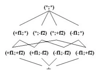
It should be easy to see that the set S forms a Boolean lattice with the following relation among the assignments,≤_R: for any two assignmentsa1

anda2,a1 ≤R a2iff the value of every featurefi ina1is identical to the value offiina2, unlessfi is unspecified ina2. The top element of the lattice

is an assignment in which all features are unspec-ified, and the bottom is the contradiction. Every element of the lattice is amonomialcorresponding to the conjunction of the specified feature values. An example lattice for two binary features is given in Figure 1.

Figure 1: A lattice for 2 binary features

A language L consists of pairs from Σ×S0. That is, the learner is exposed to morphs in differ-ent environmdiffer-ents.

3_{However, we could also conceive of morphs as functions}

specifying what transformations apply to the stem without much change to the formalism.

One way of stating the learning problem is to say that the learner has to learn a grammar for the target language L (we would then have to spec-ify what this grammar should look like). Another way is to say that the learner has to learn the lan-guage mapping itself. We can do the latter by us-ing Boolean functions to represent the mappus-ing of each morph to a set of environments. Depending on how we state the learning problem, we might get different results. For instance, it’s known that some subsets of DNF’s are not learnable, while the Boolean functions corresponding to them are learnable (Valiant, 1984). Since I will use Boolean functions for some of the learners below, I intro-duce the following notation. Let B be the set of Boolean functions mapping elements ofS0totrue orfalse. For convenience, we say that bm corre-sponds to a Boolean function that maps a set of en-vironments totrue when they are associated with

minL, and tofalseotherwise.

3 Learning Algorithms

3.1 Learner 1: an extension of the Valiant k-DNF learner

An observation that a morphological paradigm can be represented as a partition of environments in which each block corresponds to a mapping be-tween a morph and a DNF, allows us to easily con-vert standard DNF learning algorithms that rely on positive and negative examples into paradigm-learning algorithms that rely on positive examples only. We can do that by iteratively applying any DNF learning algorithm treating instances of in-put pairs like (m, e) as positive examples for m

and as negative examples for all other morphs. Below, I show how this can be done by ex-tending ak-DNF4 learner of (Valiant, 1984) to a paradigm-learner. To handle cases of free varia-tion we need to keep track of what morphs occur in exactly the same environments. We can do this by defining the partitionΠon the input following the recipe in (1) (substituting environments for the variabler).

The original learner learns from negative exam-ples alone. It initializes the hypothesis to the dis-junction of all possible condis-junctions of length at mostk, and subtracts from this hypothesis mono-mials that are consistent with the negative ex-amples. We will do the same thing for each

4_{k-DNF formula is a formula with at mostkfeature}

morph using positive examples only (as described above), and forgoing subtraction in a cases of free-variation. The modified learner is given below. The following additional notation is used: Lexis the lexicon or a hypothesis. The formula D is a disjunction of all possible conjunctions of length at mostk. We say that two assignments are con-sistentwith each other if they agree on all specified features. Following standard notation, we assume that the learner is exposed to some textTthat con-sists of an infinite sequence of (possibly) repeating elements fromL. tj is a finite subsequence of the first j elements from T. L(tj) is the set of ele-ments intj.

Learner 1 (input:tj)

1. set Lex := {hm, Di| ∃hm, ei ∈ L(tj)}

2. For each hm, ei ∈ L(tj), for each

m0 s.t. ¬∃ block bl ∈ Π ofL(tj),

hm, ei ∈blandhm0, ei ∈bl: replace hm0, fi in Lex by hm0, f0i

where f0 is the result of removing every monomial consistent withe.

This learner initially assumes that every morph can be used everywhere. Then, when it hears one morph in a given environment, it assumes that no other morph can be heard in exactly that environ-ment unless it already knows that this environenviron-ment permits free variation (this is established in the partitionΠ).

4 Learner 2:

The next learner is an elaboration on the previous learner. It differs from it in only one respect: in-stead of initializing lexical representations of ev-ery morph to be a disjunction of all possible mono-mials of length at mostk, we initialize it to be the disjunction of all and only those monomials that are consistent with some environment paired with the morph in the language. This learner is simi-lar to the DNF learners that do something on both positive and negative examples (see (Kushilevitz and Roth, 1996; Blum, 1992)).

So, for every morphmused in the language, we define a disjunction of monomialsDmthat can be derived as follows. (i) LetEmbe the enumeration of all environments in which m occurs in L (ii) letMicorrespond to a set of all subsets of feature

values inei,ei ∈E(iii) letDm beWM, where a sets∈M iffs∈Mi, for somei.

Learner 2 can now be stated as a learner that is identical to Learner 1 except for the initial set-ting of Lex. Now, Lex will be set to Lex :=

{hm, Dmi| ∃hm, ei ∈L(ti)}.

Because this learner does not require enumer-ation of all possible monomials, but just those that are consistent with the positive data, it can handle “polynomially explainable” subclass of DNF’s (for more on this see (Kushilevitz and Roth, 1996)).

5 Learner 3: a learner biased towards monomial and elsewhere distributions

Next, I present a batch version of a learner I pro-posed based on certain typological observations and linguists’ insights about blocking. The typo-logical observations come from a sample of verbal agreement paradigms (Pertsova, 2007) and per-sonal pronoun paradigms (Cysouw, 2003) show-ing that majority of paradigms have either “mono-mial” or “elsewhere” distribution (defined below). Roughly speaking, a morph has a monomial dis-tribution if it can be described with a single mono-mial. A morph has an elsewhere distribution if this distribution can be viewed as a complement of distributions of other monomial or elsewhere-morphs. To define these terms more precisely I need to introduce some additional notation. Let

T

ex be the intersection of all environments in which morphxoccurs (i.e., these are the invariant features ofx). This set corresponds to a least up-per bound of the environments associated withxin the latticehS,≤Ri, call itlubx. Then, let the min-imal monomial function for a morph x, denoted

mmx, be a Boolean function that maps an envi-ronment to trueif it is consistent withlubx and to f alseotherwise. As usual, an extension of a Boolean function, ext(b) is the set of all assign-ments thatbmaps to true.

(2) Monomial distribution

A morphxhas a monomial distribution iff

bx ≡mmx.

en-vironments in the language.

(3) Elsewhere distribution

A morphx has an elsewhere distribution iffbx ≡mmx−(mmx1 ∨mmx2 ∨. . .∨

(mmxn))for allxi 6=xinΣ.

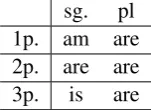
The definition above amounts to saying that a morph has an elsewhere distribution if the envi-ronments in which it occurs are in the extension of its minimal monomial function minus the min-imal monomial functions of all other morphs. An example of a lexical item with an elsewhere distri-bution is the present tense formareof the verb “to be”, shown below.

Table 1: The present tense of “to be” in English

sg. pl 1p. am are 2p. are are 3p. is are

Elsewhere morphemes are often described in linguistic accounts by appealing to the notion of blocking. For instance, the lexical representation of are is said to be unspecified for both person and number, and is said to be “blocked” by two other forms: am and is. My hypothesis is that the reason why such non-monotonic analyses ap-pear so natural to linguists is the same reason for why monomial and elsewhere distributions are ty-pologically common: namely, the learners (and, apparently, the analysts) are prone to generalize the distribution of morphs to minimal monomi-als first, and later correct any overgeneralizations that might arise by using default reasoning, i.e. by positing exceptions that override the general rule. Of course, the above strategy alone is not sufficient to capture distributions that are neither monomial, nor elsewhere (I call such distributions “overlap-ping”, cf. the suffixes -en and -tin the German paradigm in Table 2), which might also explain why such paradigms are typologically rare.

Table 2: Present tense of some regular verbs in German

sg. pl 1p. -e -en 2p. -st -t 3p. -t -en

The original learner I proposed is an incre-mental learner that calculates grammars similar to those proposed by linguists, namely grammars consisting of a lexicon and a filtering “blocking” component. The version presented here is a sim-pler batch learner that learns a partition of Boolean functions instead.5 _{Nevertheless, the main} proper-ties of the original learner are preserved: specifi-cally, a bias towards monomial and elsewhere dis-tributions.

To determine what kind of distribution a morph has, I define a relationC. A morphm stands in a relation Cto another morph m0 if ∃hm, ei ∈ L, such that lubm0 is consistent with e. In other

words, mCm0 if m occurs in any environment consistent with the invariant features ofm0. Let

C+be a transitive closure ofC.

Learner 3 (input:tj)

1. LetS(tj)be the set of pairs intj containing monomial- or elsewhere-distribution morphs. That is, hm, ei ∈ S(tj) iff ¬∃m0 such that

mC+m0andm0C+m.

2. LetO(tj) = tj −S(tj)(the set of all other pairs).

3. A pair hm, ei ∈ S is a least element of S

iff ¬∃hm0, e0i ∈ (S − {hm, ei}) such that

m0C+m.

4. Given a hypothesisLex, and for any expres-sionhm, ei ∈ Lex: letrem((m, e), Lex) = (m,(mmm− {b|hm0, bi ∈Lex}))6

1. setS:=S(tj)andLex:=∅

2. While S 6= ∅: remove a least x

from S and set Lex := Lex ∪ rem(x, Lex)

3. SetLex:=Lex∪O(tj).

This learner initially assumes that the lexicon is empty. Then it proceeds adding Boolean functions corresponding to minimal monomials for morphs that are in the setS(tj)(i.e., morphs that have ei-ther monomial or elsewhere distributions). This

5_{I thank Ed Stabler for relating this batch learner to me}

(p.c.).

6_{For any two Boolean functionsb, b}0

:b−b0is the function that mapseto 1 iffe ∈ext(b)ande 6∈ext(b0). Similarly,

b+b0 is the function that mapseto 1 iffe ∈ ext(b)and

is done in a particular order, namely in the or-der in which the morphs can be said to block each other. The remaining text is learned by rote-memorization. Although this learner is more com-plex than the previous two learners, it generalizes fast when applied to paradigms with monomial and elsewhere distributions.

5.1 Learner 4: a learner biased towards shorter formulas

Next, I discuss a learner for morphological paradigms, proposed by another linguist, David Adger. Adger describes his learner informally showing how it would work on a few examples. Below, I formalize his proposal in terms of learn-ing Boolean partitions. The general strategy of this learner is to consider simplest monomials first (those with the fewer number of specified features) and see how much data they can unambiguously and non-redundantly account for. If a monomial is consistent with several morphs in the text - it is discarded unless the morphs in question are in free variation. This simple strategy is reiterated for the next set of most simple monomials, etc.

Learner 4 (inputtj)

1. Let Mi be the set of all monomials over F withispecified features.

2. LetBi be the set of Boolean functions from environments to truth values corresponding toMi in the following way: for each mono-mial mn ∈ Mi the corresponding Boolean function b is such that b(e) = 1 if e is an environment consistent with mn; otherwise

b(e) = 0.

3. Uniqueness check:

For a Boolean functionb, morphm, and text

tj let unique(b, m, tj) = 1 iff ext(bm) ⊆

ext(b) and ¬∃hm0, ei ∈ L(tj), s.t. e ∈

ext(b)ande6∈ext(bm).

1. setLex:= Σ× ∅andi:= 0;

2. while Lex does not correspond to

L(tj)ANDi≤ |F|do:

for each b ∈ Bi, for each m, s.t.

∃hm, ei ∈L(tj):

• ifunique(b, m, tj) = 1then replacehm, fi withhm, f +bi

inLex

i←i+ 1

This learner considers all monomials in the or-der of their simplicity (determined by the num-ber of specified features), and if the monomial in question is consistent with environments associ-ated with a unique morph then these environments are added to the extension of the Boolean function for that morph. As a result, this learner will con-verge faster on paradigms in which morphs can be described with disjunctions of shorter monomials since such monomials are considered first.

6 Comparison

6.1 Basic properties

First, consider some of the basic properties of the learners presented here. For this purpose, we will assume that we can apply these learners in an iter-ative fashion to larger and larger batches of data. We say that a learner is consistentif and only if, given a texttj, it always converges on the gram-mar generating all the data seen in tj (Osherson et al., 1986). A learner ismonotonic if and only if for every texttand every point j < k, the hy-pothesis the learner converges on attj is a subset of the hypothesis at tk (or for learners that learn by elimination: the hypothesis at tj is a superset of the hypothesis attk). And, finally, a learner is generalizingif and only if for sometjit converges on a hypothesis that makes a prediction beyond the elements oftj.

The table below classifies the four learners ac-cording to the above properties.

Learner consist. monoton. generalizing Learner 1 yes yes yes

Learner 2 yes yes yes Learner 3 yes no yes Learner 4 yes yes yes

6.2 Illustration

To demonstrate how the learners work, consider this simple example. Suppose we are learning the following distribution of morphsA andB over 2 binary features.

(4) Example 1

+f1 −f1

+f2 A B

−f2 B B

Suppose further that the textt3is:

A +f1; +f2

B −f1; +f2

B +f1;−f2

Learner 1 generalizes right away by assuming that every morph can appear in every environment which leads to massive overgeneralizations. These overgeneralizations are eventually eliminated as more data is discovered. For instance, after pro-cessing the first pair in the text above, the learner “learns” that B does not occur in any environ-ment consistent with(+f1; +f2)since it has just seenA in that environment. After processingt3,

Learner 1 has the following hypothesis:

A (+f1; +f2)∨(−f1;−f2)

B (−f1)∨(−f2)

That is, after seeingt3, Learner 2 correctly

pre-dicts the distribution of morphs in environments that it has seen, but it still predicts that both A

and B should occur in the not-yet-observed en-vironment, (−f1;−f2). This learner can some-times converge before seeing all data-points, es-pecially if the input includes a lot of free varia-tion. If fact, if in the above exampleAandBwere in free variation in all environments, Learner 1 would have converged right away on its initial set-ting of the lexicon. However, in paradigms with no free variation convergence is typically slow since the learner follows a very conservative strategy of learning by elimination.

Unlike Learner 1, Learner 2 will converge after seeingt3. This is because this learner’s initial

pothesis is more restricted. Namely, the initial hy-pothesis for Aincludes disjunction of only those monomials that are consistent with (+f1; +f2). Hence,Ais never overgeneralized to(−f1;−f2). Like Learner 1, Learner 2 also learns by

elimina-tion, however, on top of that it also restricts its ini-tial hypothesis which leads to faster convergence.

Let’s now consider the behavior of learner 3 on example 1. Recall that this learner first computes minimal monomials of all morphs, and checks in they have monomial or elsewhere distributions (this is done via the relationC+). In this case,A

has a monomial distribution, and B has an else-where distribution. Therefore, the learner first computes the Boolean function forAwhose exten-sion is simply (+f1; +f2); and then the Boolean function forB, whose extension includes environ-ments consistent with (*;*) minus those consistent with(+f1; +f2), which yields the following hy-pothesis:

ext(bA) [+f1; +f2]

ext(bB) [−f1; +f2][+f1;−f2][−f1;−f2]

That is, Learner 3 generalizes and converges on the right language after seeing textt3.

Learner 4 also converges at this point. This learner first considers how much data can be un-ambiguously accounted for with the most minimal monomial (*;*). Since bothAandB occur in en-vironments consistent with this monomial, noth-ing is added to the lexicon. On the next round, it considers all monomials with one specified fea-ture. 2 such monomials, (−f1) and(−f2), are consistent only withB, and so we predictBto ap-pear in the not-yet-seen environment(−f1;−f2). Thus, the hypothesis that Learner 4 arrives at is the same as the hypothesis Learners 3 arrives at after seeingt3.

6.3 Differences

While the last three learners perform similarly on the simple example above, there are significant differences between them. These differences be-come apparent when we consider larger paradigms with homonymy and free variation.

First, let’s look at an example that involves a more elaborate homonymy than example 1. Con-sider, for instance, the following text.

(5) Example 2

A [+f1; +f2; +f3]

A [+f1;−f2;−f3]

A [+f1; +f2;−f3]

A [−f1; +f2; +f3]

Given this text, all three learners will differ in their predictions with respect to the environ-ment (−f1; +f2;−f3). Learner 2 will pre-dict both A and B to occur in this environment since not enough monomials will be removed from representations of A or B to rule out ei-ther morph from occurring in (−f1; +f2;−f3). Learner 3 will predict A to appear in all envi-ronments that haven’t been seen yet, including

(−f1; +f2;−f3). This is because in the cur-rent text the minimal monomial for Ais (∗;∗;∗)

and A has an elsewhere distribution. On the other hand, Learner 4 predicts B to occur in

(−f1; +f2;−f3). This is because the exten-sion of the Boolean function for B includes any environments consistent with(−f1;−f3)or

(−f1;−f2)since these are the simplest monomi-als that uniquely pick outB.

Thus, the three learners follow very different generalization routes. Overall, Learner 2 is more cautious and slower to generalize. It predicts free variation in all environments for which not enough data has been seen to converge on a single morph. Learner 3 is unique in preferring monomial and elsewhere distributions. For instance, in the above example it treatsAas a ‘default’ morph. Learner 4 is unique in its preference for morphs describ-able with disjunction of simpler monomials. Be-cause of this preference, it will sometimes gener-alize even after seeing just one instance of a morph (since several simple monomials can be consistent with this instance alone).

One way to test what the human learners do in a situation like the one above is to use artifi-cial grammar learning experiments. Such experi-ments have been used for learning individual con-cepts over features like shape, color, texture, etc. Some work on concept learning suggests that it is subjectively easier to learn concepts describable with shorter formulas (Feldman, 2000; Feldman, 2004). Other recent work challenges this idea (La-fond et al., 2007), showing that people don’t al-ways converge on the most minimal representa-tion, but instead go for the more simple and gen-eral representation and learn exceptions to it (this approach is more in line with Learner 3).

Some initial results from my pilot experiments on learning partitions of concept spaces (using ab-stract shapes, rather than language stimuli) also suggest that people find paradigms with else-where distributions easier to learn than the ones

with overlapping distributions (like the German paradigms in 2). However, I also found a bias to-ward paradigms with the fewer number of relevant features. This bias is consistent with Learner 4 since this learner tries to assume the smallest num-ber of relevant features possible. Thus, both learn-ers have their merits.

Another area in which the considered learn-ers make somewhat different predictions has to do with free variation. While I can’t discuss this at length due to space constraints, let me comment that any batch learner can easily de-tect free-variation before generalizing, which is exactly what most of the above learners do (ex-cept Learner 3, but it can also be changed to do the same thing). However, since free variation is rather marginal in morphological paradigms, it is possible that it would be rather problem-atic. In fact, free variation is more problematic if we switch from the batch learners to incremental learners.

7 Directions for further research

There are of course many other learners one could consider for learning paradigms, including ap-proaches quite different in spirit from the ones considered here. In particular, some recently pop-ular approaches conceive of learning as matching probabilities of the observed data (e.g., Bayesian learning). Comparing such approaches with the algorithmic ones is difficult since the criteria for success are defined so differently, but it would still be interesting to see whether the kinds of prior assumptions needed for a Bayesian model to match human performance would have some-thing in common with properties that the learn-ers considered here relied on. These properties include the disjoint nature of paradigm cells, the prevalence of monomial and elsewhere morphs, and the economy considerations. Other empirical work that might help to differentiate Boolean par-tition learners (besides typological and experimen-tal work already mentioned) includes finding rele-vant language acquisition data, and examining (or modeling) language change (assuming that learn-ing biases influence language change).

References

Avrim Blum. 1992. Learning Boolean functions in an infinite attribute space. Machine Learning, 9:373– 386.

Michael Cysouw. 2003. The Paradigmatic Structure of Person Marking. Oxford University Press, NY.

Jacob Feldman. 2000. Minimization of complexity in human concept learning. Nature, 407:630–633.

Jacob Feldman. 2004. How surprising is a simple pat-tern? Quantifying ‘Eureka!’. Cognition, 93:199– 224.

John Goldsmith. 2001. Unsupervised learning of a morphology of a natural language. Computational Linguistics, 27:153–198.

Anthony Kroch. 1994. Morphosyntactic variation. In Katharine Beals et al., editor, Papers from the 30th regional meeting of the Chicago Linguistics Soci-ety: Parasession on variation and linguistic theory. Chicago Linguistics Society, Chicago.

Eyal Kushilevitz and Dan Roth. 1996. On learning vi-sual concepts and DNF formulae. Machine Learn-ing, 24:65–85.

Daniel Lafond, Yves Lacouture, and Guy Mineau. 2007. Complexity minimization in rule-based cat-egory learning: revising the catalog of boolean con-cepts and evidence for non-minimal rules. Journal of Mathematical Psychology, 51:57–74.

Gary Marcus, Steven Pinker, Michael Ullman, Michelle Hollander, T. John Rosen, and Fei Xu. 1992. Overregularization in language acquisition.

Monographs of the Society for Research in Child Development, 57(4). Includes commentary by Harold Clahsen.

Robert M. Nosofsky, Thomas J. Palmeri, and S.C. McKinley. 1994. Rule-plus-exception model of classification learning. Psychological Review, 101:53–79.

Daniel Osherson, Scott Weinstein, and Michael Stob. 1986. Systems that Learn. MIT Press, Cambridge, Massachusetts.

Katya Pertsova. 2007. Learning Form-Meaning Map-pings in the Presence of Homonymy. Ph.D. thesis, University of California, Los Angeles.

Jeffrey Mark Siskind. 1996. A computational study of cross-situational techniques for learning word-to-meaning mappings. Cognition, 61(1-2):1–38, Oct-Nov.

Matthew G. Snover, Gaja E. Jarosz, and Michael R. Brent. 2002. Unsupervised learning of morphology using a novel directed search algorithm: taking the first step. InProceedings of the ACL-02 workshop on Morphological and phonological learning, pages 11–20, Morristown, NJ, USA. Association for Com-putational Linguistics.

Leslie G. Valiant. 1984. A theory of the learnable.

CACM, 17(11):1134–1142.