Faculty of Electrical Engineering,
Mathematics & Computer Science
Automatic annotation
of the cooking process
Jan Ubbo van Baardewijk Master thesis
February 2018
Supervisors:
When looking for an interesting subject to write my master thesis about, I visited TNO Soesterberg to meet Anne-Marie. Automatic annotation of a cooking experiment was suggested as one of the subjects for my the thesis. It turned out to be a very interesting topic which offered more than enough possibilities for extensive research. I want to thank TNO to give me this opportunity. And I want to thank Anne-Marie Brouwer for supporting me a lot. Thanks Mannes to be my supervisor from the University of Twente, you had no doubt that I would succeed.
Bedankt Inge, mijn aanstaande vrouw, voor alle mentale support, liefde en geduld. Ook mijn ouders wil ik bedanken, niet in de minste plaats omdat ik tijdens mijn peri-ode bij TNO weer tijdelijk bij hen in kon trekken. Tenslotte wil ik God bedanken die dit alles mogelijk heeft gemaakt.
Automatic annotation of actions using accelerometer data would make the analysis of everyday, spontaneous activities much easier. It could create a context when try-ing to relate physiology to experience and it could lead to extracttry-ing new features. The goal of this thesis is to examine how different actions can be classified using inertial measurement unit data and to see how well a model that is trained in a struc-tured experiment could be used to classify actions in a more naturalistic setting. This is done in the context of food preparation, because the project ’Quantified consumer’ is used as the framework.
Therefore, the data from ’Quantified consumer’ is used as the data set for this experiment. We chose an approach where we split the data in windows of 1 second and classify each window. As the ground truth we used a selection of the data set for which we could be sure about the performed action. We performed three different classification tasks, each with a different number of actions. k-nearest neighbor with k=5 was used as classification method with up to 6 different features. The informa-tion from neighboring windows were taken into account for each of the windows.
Classification between action and standing still had a high performance, classifi-cation with more classes gave the highest results on the dry cooking session data. A model trained on dry cooking data and run on real cooking data performed almost as well as a model trained on real cooking data, provided that the dry cooking set is balanced between classes.
This study presented a way to evaluate different action recognition models with-out requiring manual annotation of videos.
To improve the results, we could look at increasing the number of neighboring windows that is taken into account or better look at the used features. A different classification method like deep learning hopefully improves recognition performance as well as a more user-specific approach.
Preface iii
Summary v
List of acronyms xi
1 Introduction 1
1.1 Context . . . 1
1.2 Problem statement . . . 2
1.3 Research questions . . . 3
1.4 Overview of this paper . . . 4
2 Related work 5 2.1 Automatic annotation . . . 5
2.1.1 Activity types . . . 5
2.1.2 Input . . . 5
2.1.3 Output . . . 6
2.2 Preprocessing and feature extraction . . . 6
2.2.1 Data windowing . . . 7
2.2.2 Labeling activity data . . . 8
2.2.3 Feature extraction . . . 9
2.2.4 Filtering . . . 12
2.2.5 Principal component analysis . . . 12
2.2.6 Normalization . . . 12
2.2.7 Neighboring windows . . . 13
2.3 Action segmentation and recognition methods . . . 14
2.3.1 Possible approaches for automatic annotation of actions . . . . 14
2.3.2 Classification methods . . . 16
2.3.3 Classification tools . . . 16
2.3.4 Comparison . . . 17
2.4 Evaluation . . . 17
2.4.1 Introduction . . . 17
2.4.2 Splitting data set . . . 18
2.4.3 Evaluation measure . . . 18
3 Data set 21 3.1 Data quality . . . 26
4 Methodology 27 4.1 Approach . . . 27
4.2 Data windowing . . . 27
4.3 Ground truth . . . 28
4.3.1 Selection . . . 29
4.4 Classification tasks . . . 29
4.5 Splitting train, validation and test set . . . 30
4.6 Tests . . . 30
4.7 Evaluation . . . 31
4.8 Classification method . . . 31
4.9 Features . . . 32
4.10 Balancing train set . . . 32
5 Results 33 5.1 Two classes: Standing still and action . . . 33
5.2 Three classes: Standing still, stirring and pressing button . . . 34
5.3 Four classes: Standing still, stirring, adding and pressing button . . . . 38
5.3.1 Selected data . . . 38
5.3.2 All data . . . 43
6 Discussion 45 6.1 ’Action’ versus ’standing still’ . . . 45
6.1.1 Classification performance . . . 45
6.1.2 Generalization dry to real . . . 45
6.2 Multiple classes . . . 46
6.2.1 Classification performance . . . 46
6.2.2 Generalization dry to real . . . 48
7 Conclusion and recommendations 51 7.1 Conclusion . . . 51
7.2 Improving the performance of the models . . . 51
Appendices
A Data selection 57
A.1 Class ’standing still’ . . . 57
A.2 Class ’Stirring’ . . . 57
A.3 Class ’Pouring’ . . . 58
A.4 Class ’Pressing button’ . . . 58
A.5 Class ’Adding bowl’ . . . 59
AAL ambient assisted living ADL activity of daily living BN Bayesian network DNN deep neural network DT decision tree
ECG electrocardiography EEG electroencephalography FFT fast Fourier transform
FNSW fixed-size non-overlapping sliding window FOSW fixed-size overlapping sliding window HMM hidden Markov model
IMU inertial measurement unit k-NN k-nearest neighbor
LOOCV leave-one-out cross-validation NB naive Bayes
PSD power spectral density
PCA principal component analysis RF random (decision) forest RMS root mean square
SMA signal magnitude area
Introduction
Studying everyday, spontaneous activities often requires annotation of the actions that are performed during the activity. These annotations are usually done manu-ally, which takes a lot of time and effort. Automatic annotation of actions using ac-celerometer data would make the analysis of this type of data much easier. Training annotation models could be facilitated by using data from a structured experiment and use these models for automatic annotation on the data of interest in a more naturalistic setting.
This thesis will examine how different actions can be classified using inertial measurement unit (IMU) data and how well we can generalize a model that is trained in a structured experiment to a more naturalistic setting.
1.1 Context
In the project ’Quantified consumer’ at TNO, the goal is to estimate the experienced emotion during real-life cooking and tasting. Positive emotions are critical for the success of food products in the marketplace, but little is known about the emotional processes in the interaction of the consumer with the product during food preparation and cooking. New methods to quantify these experiences are essential in order to successfully deliver emotional benefits and health to consumers by making nutritious cooking and eating desirable, enjoyable and easy to understand and do.
Therefore, an experiment is done where participants are asked to cook a dish, which is cooked with either presumably pleasant products (fresh ingredients and nice-looking packaging) or less pleasant products. During the experiment, physio-logical measurements such as electroencephalography (EEG), electrocardiography (ECG), skin conductance and IMU data (accelerometer and gyroscope) are recorded. The participants follow prerecorded, auditory instructions given at specified times that guide them through the cooking process. Before and after the real cooking
session, a so-called ’dry cooking’ session is run where participants simulate the movements of real cooking.
We aim to automatically annotate the actions of the cooking process in this con-text, using the IMU data. A few studies about the automatic annotation of sensor data from subjects preparing food have been done in the past, mainly [1], [2] and [3]. In these studies both video and IMU data were recorded and used to perform auto-matic annotation.
Because the project ’Quantified consumer’ is used as the framework, the focus of this paper is on automatic annotation of sensor data from subjects preparing food. However, automatic annotation would facilitate research in a large range of real-life conditions.
1.2 Problem statement
Annotation of the actions (whether automatic or manual) helps with the interpre-tation of physiological measurements in experiments like ’Quantified consumer’: It is possible to relate physiological reactions (caused by motor activity and emotion) to action more precisely by looking where an action started and where a reaction should occur, instead of looking at the start of the commando given through the ex-perimental setup. In this way, it is creating a context when trying to relate physiology to experience.
Another benefit from annotation is that it could lead to extracting new, potentially interesting features, such as movement duration, or the duration of stirring.
Currently, in order to annotate the actions, many experiments need to have a very structured setup, where subjects are explicitly instructed at a certain time stamp to perform certain actions, so that the data is labeled. Experiments that do not require the subjects to execute the experiment in a very structured order, but instead execute the activity at their own pace, make the setting more naturalistic. However, this kind of experiment requires manual annotation, which requires one or more experts to inspect the data and label the data with the actions that the subject is doing, which is very time-consuming work.
An automatic annotation system, based on an action recognition model that would detect and identify the separate actions that are performed, would greatly facilitate the analysis of naturalistic experiments.
of their actions, could help in monitoring these people.
Many experiments that train action recognition models, (such as [4] and [5]) are very structured. In these experiments, participants are performing one action at a time so it is easy to generate a ground truth. However, it is questionable whether models trained in these artificial settings generalize to real life conditions, where actions may be performed differently.
Other experiments that try to model action recognition models are less structured and use a more naturalistic setting (such as [1] and [2]), but require precise manual annotation, which is usually a lot of work.
An important part of this thesis is to explore how data from a structured experi-ment could be used to automatically annotate a more naturalistic experiexperi-ment. This is not seen in other studies where either data from an experiment with a structured setup is used or data from an experiment with a manually annotated, naturalistic setup is used for training and testing of the action recognition model.
This could be very interesting in an experiment with a naturalistic setting where a calibration session could be done prior to the experiment. Most experiments consist of their own set of actions and therefore require a unique model in order to recognize all actions. In the calibration session, the model is trained for all of these actions in a very structured setting and then used to classify the real sessions that follow. This could make the process of automatic annotation less complicated to apply in practice.
1.3 Research questions
In order to facilitate the automatic annotation of actions, this paper will examine the possibilities to classify the actions, using a supervised model that is trained on IMU data. More specifically we will look at data of participants who cooked a dish, provided by TNO from the experiment ’Quantified consumer’. Therefore the main question of this project is:
How well can we automatically annotate the actions in a cooking process, based on the IMU data, using a supervised model?
In order to classify all actions, we need to know where in the data the participant is standing still and where he is performing an action. Therefore, we will first look into the binary classification of the data into action and no action, which leads to the following question:
For the active parts, we will look which actions are performed. A multi-class classifi-cation model will be trained in order to classify most of the actions that are performed by the participants during cooking.
What is the performance of a model trained on IMU data for classification of cooking data into multiple actions?
In extension, we will look how we can use data from a more structured experiment for automatic annotation of data from an experiment that has a more naturalistic setting. There is data from two sessions: a dry cooking session that is strongly structured and a real cooking session where participants cooked a real dish, which was less structured. It would be interesting to know how well dry cooking data generalizes to real cooking. This leads to the following question:
How does the classification performance of a model trained on dry cook-ing data compare to a model trained on real cookcook-ing data for the classifi-cation of actions in real cooking data?
1.4 Overview of this paper
Related work
2.1 Automatic annotation
A considerable amount of research has been done in the past on the automatic annotation of human activities, such as food preparation. This section describes in general the type of activities that have been automatically classified, the input that is required and the output that is expected after automatic annotation. The details of the process are described in later sections.
2.1.1 Activity types
Cornacchia et al. [6] give an overview of existing studies on activity detection and classification. In their overview, they group human activities into two types: global body movement and local interaction. The first type includes activities like walking, running, jumping and swimming, the second type consists of activities like cleaning, eating, construction, food preparation and office activities.
This paper focuses on the second type, which means our studied literature will fo-cus mostly on research towards local interaction recognition, especially food prepa-ration. However, papers about the first type will be mentioned as well, as these papers could provide useful insights.
2.1.2 Input
Automatic annotation of human activities can be done on different kinds of sensor data. The survey of activity recognition studies provided in [6] distinguishes various types of sensor types: Accelerometer and/or gyroscope (often combined into an IMU) are mostly used for global body movement activities, while camera systems are often used for local interaction. Hybrid sensor systems, such as camera combined with an IMU, are often used for a combination of these activity types. However,
some studies explored the possibilities of recognition of local interaction using only IMU data. We will further focus on these possibilities for annotating IMU data.
The extraction of features from the sensor data is required as input to the classi-fier. They need to be chosen in such a way that the classifier can detect and classify the different actions. More details about the different features that are commonly used for activity detection and classification are in subsection 2.2.3.
Other input that is required is the ground truth, both for training a classifier and for evaluation. The most precise way to correctly label spontaneous activities can probably be provided by one or more human experts. Video data could be useful for this. After the model for automatic annotation has been created, hopefully the manual labeling will not be necessary anymore.
2.1.3 Output
Two things are expected after automatic annotation: actions are detected and the detected actions are recognized and labeled with the corresponding action.
Detecting where an action begins and where it ends is often called (temporal) segmentation. To do this automatically, a change in the performed action should be detected in the IMU data. Based on these detected changes, the data is segmented into actions. The time between actions should also be labeled as non-action, so that all data is labeled (either as an action or non-action).
Recognition of actions is the identification of an action from sensor data. It should be possible to annotate an action with the corresponding action label.
Segmentation and recognition can be done sequentially, but there are methods that combine these two. Possible approaches to this are described in more detail in section 2.3.
In the end, the output of the annotation process should be a labeled data set, where the labels are those of the actions and non-actions, with the exact points in time where actions start and end.
2.2 Preprocessing and feature extraction
2.2.1 Data windowing
In order to process all the data, it is often necessary to split up the data into smaller chunks or windows. There are multiple methods to do this and very different choices for window size are made.
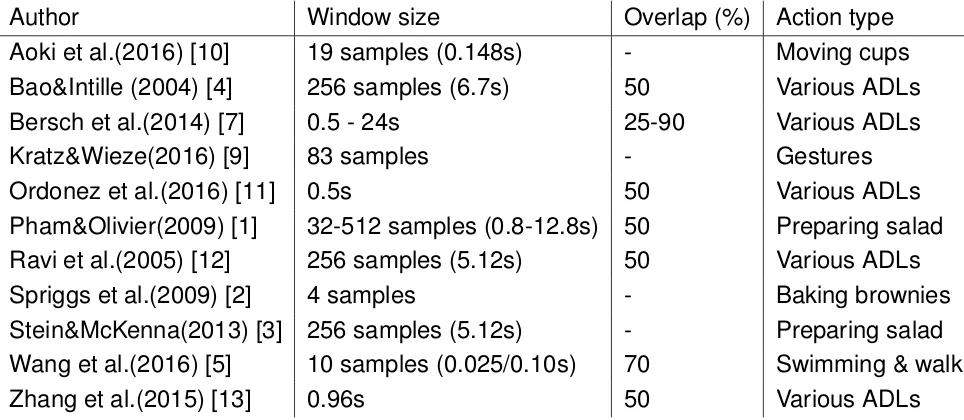
Bersch et al. [7] state that many studies base their windowing method and win-dow size on previous experiments, hardware limitations, or do not state a specific reason. They give an overview of research projects on classification of activities of daily living (ADLs) using accelerometer data and describe several different window-ing techniques used in these projects, of which three in particular: fixed-size non-overlapping sliding window (FNSW), fixed-size non-overlapping sliding window (FOSW) (with various overlap percentages and sliding window) and, finally, bottom-up. Win-dow sizes that are used vary between 0.25 and 74s, but this depends on the type of activity: a small window size is often selected in studies with faster-changing activ-ities like walking and standing and larger window sizes are selected in studies with activities that are not changing very quickly, like making coffee or eating breakfast.
Their study was done to make a more informed decision on such parameter selection. Bersch et al. did an experiment with 32 different window sizes on two datasets, one dataset [4] consisting of subjects performing ADLs, such as walking, sitting, walking and carrying an item, standing still, lying down, and climbing stairs. Activities that were used from the other dataset [8] were stand, walk, sit, and lie. Different methods for windowing the data were tested as well. They looked at the classification accuracy of predicting the activity class for each of the instances for different parameters. In the results, FOSW with 90% overlap gave the highest accu-racy out of all windowing methods for both datasets. The optimal choice of window size was different per dataset. For the first dataset, a window size of 6.5 to 11s resulted in the best accuracy, for the other dataset, a window size <1.5s gave the best results.
Spriggs et al. [2], a study about the classification of subjects baking brownies, took the mean of every 4 sample window to smooth and down-sample the sensor data.
Kratz&Wieze [9] tried to segment mobile device gestures by classifying data points into four different classes: noise, start, middle and end. For online segmen-tation, they chose a sliding window approach. As the size of the sliding window they chose 83 data points, the rounded up average of gesture phase segment length. Because of the large number of potential training sample, they took every 100th window for the training of the classifiers.
Author Window size Overlap (%) Action type Aoki et al.(2016) [10] 19 samples (0.148s) - Moving cups Bao&Intille (2004) [4] 256 samples (6.7s) 50 Various ADLs
Bersch et al.(2014) [7] 0.5 - 24s 25-90 Various ADLs
Kratz&Wieze(2016) [9] 83 samples - Gestures
Ordonez et al.(2016) [11] 0.5s 50 Various ADLs
Pham&Olivier(2009) [1] 32-512 samples (0.8-12.8s) 50 Preparing salad Ravi et al.(2005) [12] 256 samples (5.12s) 50 Various ADLs
Spriggs et al.(2009) [2] 4 samples - Baking brownies
Stein&McKenna(2013) [3] 256 samples (5.12s) - Preparing salad Wang et al.(2016) [5] 10 samples (0.025/0.10s) 70 Swimming & walking
[image:20.595.66.548.86.296.2]Zhang et al.(2015) [13] 0.96s 50 Various ADLs
Table 2.1: Comparison of window sizes and overlap used in existing studies.
2.2.2 Labeling activity data
All methods that use supervised learning require the labeling (or annotation) of the data as a ground truth. Different labels can be given to the data, depending on what the model should predict. For action segmentation, these labels should only be the points where the action is changing. Aoki et al. [10] call these points ’seg-ment points’. For action recognition, the label should be the action that is currently performed.
Manual labeling is performed in order to create these labeling sets. In one study [10] where subjects were moving cups on a table (some kind of local interaction), manual annotation of the action segments is done by using the recorded video. Several observers decided where segments start and end. This was used as the ground truth for the performance analysis of the automatic segmentation.
Aoki et al. point out that a decision has to be made on the time window for which a label is given during the manual segmentation, which they call the segment range. They note that there is variation between annotators: a previous study reports there is an inter-personal error between annotators of around ±0.125s. Therefore, the
segment range used by them was 20 windows (±0.156s).
a database of people preparing salads where the annotations are exactly defined. They split up activities in three separate phases. The core phase of an activity con-sist of actions that are essential like pouring oil, while the pre- and post-phases are actions like grabbing the bottle. In this way, annotations were made unambiguous and repeatable.
When a (sliding) window is used, the class that is the ground truth has to be decided on for each window (especially when the ground truth labels are given more than once per window). Ordonez et al. [11] chose the class label at the last sample of the window.
2.2.3 Feature extraction
There are many features that can be extracted from the sensor data. However, not all of them are as useful for the classification models that we focus on here.
Bersch et al. [7] describe a number of common metrics that are used to retrieve the different features of the accelerometer sensor data in this research area. Several of these features are listed here, complemented with some features found in other relevant studies, together with a description of their use in the research field and how they are calculated.
Each of these features is modified to apply for IMU data with three axes (x, y and z). In these equations, where calculations are done for the x-axis, they can be done in the same way for the other axes. In all equations, nis the window size.
• root mean square (RMS), according to Bersch et al. used in several studies to distinguish walking patterns and in general as input to classifiers for activity recognition. The average RMS for a window is calculated using Equation 2.1;
R MSx−Axis=
s Pn
i=1x 2
i
n (2.1)
• mean signal, according to Bersch et al. used in several studies to recognize sitting and standing, to discriminate between periods of activity and rest and in general as input to various classifiers. It is calculated using Equation 2.2;
M eanx−Axis=
Pn
i=1xi
n (2.2)
• standard deviation (STD) of a signal, according to Bersch et al. extensively used in general for activity recognition, as input to various classifiers. It is calculated using Equation 2.3.
ST Dx−Axis=
s Pn
i=1(xi−M eanx−Axis)2
• signal magnitude area (SMA), according to Bersch et al. used in several stud-ies to discriminate between periods of activity and rest in order to identify peri-ods that the subject is mobilizing and when they are immobile, calculated using Equation 2.4;
SM A=
Pn
i=1(|xi| + |yi| + |zi|)
n (2.4)
• signal vector magnitude (SMV), the magnitude of the signal vector, accord-ing to Bersch et al. used in several studies to indicate degree of movement intensity and an essential metric for fall detection. Zhang et al. [13] use the magnitude of the acceleration vector as a feature for general activity classi-fication. Aoki et al. [10] use the magnitude of the angular velocity vector as the only feature for classification of local interaction. They claim that it avoids the need of a detailed kinematic model or handling IMU drift, but still gives accurate pattern recognition of human body motion.
The average magnitude of a signal vector is calculated using Equation 2.5
SMV=
Pn
i=1
q
x2
i +y
2
i+z
2
i
n (2.5)
• time-domain energy and entropy, used by Pham&Olivier [1] and Stein&McKenna [3] for classification of food preparation. Energy is calculated as shown in Equation 2.6.
T D−Ener g yx−Axis=
Pn
i=1x 2
i
n (2.6)
Pham&Olivier describe the calculation of time-domain entropy by defining a probability mass function as p(xi)=P r(X=xi), but it is unclear how they com-pute this probability function and, in extension, how they calculate their entropy feature. It is also unclear why Pham&Olivier and Stein&McKenna used these features and what the reasoning behind them is.
a certain frequency component.
P SDx−Axis(f)= |F F Tf|2 (2.7)
Frequency-domain energy is then calculated as the sum of the PSD compo-nents, divided by the window length for normalization. The DC component, which is the mean acceleration, is excluded in this sum, because that is al-ready measured by another feature. The calculation is shown in Equation 2.8. According to a paper from Nham et al. [15], this calculation follows from Par-seval’s theorem.
F D−Ener g yx−Axis=
Pn
f=1P SDx−Axis(f)
n (2.8)
Frequency-domain entropy is used for discrimination of activities with similar energy values, but with different number of dominant frequency components. Bao&Intille [4] describe it as the normalized information entropy of the PSD. The PSD is first normalized so it can be viewed as a probability density func-tion, as shown in Equation 2.9.
px−Axis(f)=PnP SDx−Axis(f)
f=1P SDx−Axis(f)
(2.9)
It is then calculated as the Shannon entropy of the PSD and divided by the maximum entropy,logn, for normalization of all values in a [0,1] interval. Effec-tively, this sets the base of the logarithm that is used for the entropy calculation to the window length. The calculation of entropy is shown in equation Equa-tion 2.10;
F D−N ormEntro p yx−Axis= −
Pn
f=1px−Axis(f) log[px−Axis(f)]
logn (2.10)
• FFTPeak. It is the intensity of the highest peak in the PSD (see Equation 2.7) and is, according to Bersch et al., used in several studies for activity recog-nition, because an activity often has a dominant frequency component, which can be characteristic for that activity;
• correlation. Zhang et al. [13] mention correlation between acceleration axes as another popular feature. Ravi et al. [12] explain that it is used to differenti-ate activities that involve translation in just one dimension from activities with translation in multiple dimensions. It is calculated between each pair of axes, as shown in Equation 2.11 for x and y:
corr(x,y)= cov(x,y)
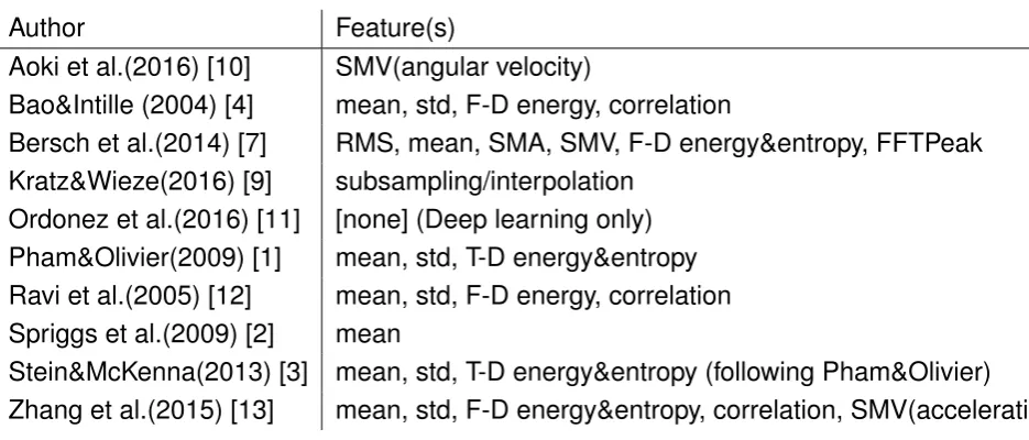
Author Feature(s)
Aoki et al.(2016) [10] SMV(angular velocity)
Bao&Intille (2004) [4] mean, std, F-D energy, correlation
Bersch et al.(2014) [7] RMS, mean, SMA, SMV, F-D energy&entropy, FFTPeak Kratz&Wieze(2016) [9] subsampling/interpolation
Ordonez et al.(2016) [11] [none] (Deep learning only) Pham&Olivier(2009) [1] mean, std, T-D energy&entropy Ravi et al.(2005) [12] mean, std, F-D energy, correlation Spriggs et al.(2009) [2] mean
Stein&McKenna(2013) [3] mean, std, T-D energy&entropy (following Pham&Olivier)
[image:24.595.67.535.82.282.2]Zhang et al.(2015) [13] mean, std, F-D energy&entropy, correlation, SMV(acceleration)
Table 2.2: Overview of features extracted from IMU data in existing studies
• subsampled values. Sometimes the data values are directly used as fea-tures and subsampled to obtain feafea-tures of homogeneous length, such as in Kratz&Wieze [9].
Table 2.2 gives an overview of all features used in several studies about activity classification.
2.2.4 Filtering
Sometimes filtering is applied to the signal to better extract several features. For example, Aoki et al. [10] apply a low-pass filter (with a cut-off frequency of 10 Hz) before calculating the angular velocity in order to filter out the noise and non-relevant components.
2.2.5 Principal component analysis
In some studies the feature space became very large. In order to reduce the size of the feature space and with that the computation time, principal component analysis (PCA) can be performed on the data. For example, Spriggs [2] reduced the number of features from 45 down to 32(or fewer) features for certain methods, using PCA.
2.2.6 Normalization
features to a certain interval, using Equation 2.12, where xi is the original feature value and x0i the new feature value:
x0i= xi−Xmin
Xmax−Xmin (2.12)
For example, Kratz&Wieze [9] mean-shifted and normalized their sensor data to a [-1,1] interval.
Another method is standardization, where all data has zero mean and unit vari-ance. Through this method, each data point is expressed in the number of standard deviations from the mean. It is calculated using Equation 2.13:
x0i= xi−Xmean
Xstd (2.13)
For example, Spriggs et al. [2] normalize all of their data with this method.
2.2.7 Neighboring windows
Information about neighboring windows could improve action detection and recog-nition. Zhang et al. [13] note that many studies only use features of the current window as input for the classifier. They claim to have improved the performance of activity recognition by using the information from neighboring windows. The features of these windows are used as additional input to the classifier in order to improve the accuracy, effectively increasing the number of features when the number of neigh-boring windows to include is increased.
For example, if 5 features are extracted from each window and one window be-fore and after the current window is incorporated in the input for the current window, the total number of features that is used for the current window is 15. They suggest that because there is interdependency between neighboring windows, incorporating this information as input when classifying improves the activity recognition perfor-mance.
Aoki et al. [10] also took a similar windowed approach where feature vectors from the adjacent time steps were concatenated to a full window, in order to incorporate temporal information. For the initial data, the first data was used in place of previous data, because there is no previous window and at the end the final data was used to pad the last window. This study investigated the influence that the choice of window size (always an odd number, because it was centered around the center window) has on the classification accuracy. A window size of 19 samples (approximately 0.148s) showed the highest accuracy.
2.3 Action segmentation and recognition methods
After preprocessing data and feature extraction, different approaches are possible towards the automatic annotation of actions in the IMU data. These are described in here as well as the classification methods most of these approaches make use of.
2.3.1 Possible approaches for automatic annotation of actions
Peak detection
This method does not use make use of a classification method, but rather detects and segments activities through analysis of the signal only. In this approach, the signal is band pass filtered at optimal frequencies in order to reveal the kinematic peaks, as is done in for example Nyugen et al. [16] for global body movement activi-ties. In order to differentiate between standing up and sitting down, they augmented the information about the peak of the acceleration with the derivative of the acceler-ation. In this way, the could detect different activities. The transitions (beginning and end) of these activities were then identified by locating the minimum or maximum to the left or right of the activity peaks.
Combined segmentation and recognition
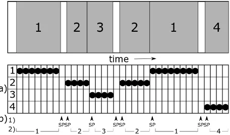
All windows are labeled as belonging to a certain type of action (or non-action). Each window is classified separately by a classification algorithm. By detecting a type of actions for each window, the data is segmented at the same time, because windows where the classified action has changed from the classified action in the previous window are then the segment points, as shown in approach a of Figure 2.1. This is the method that is used in [2].
Segmentation, then recognition
could lead to a new method for action recognition and could possibly be adapted to use for a windowed approach. It is visualized as approach b in Figure 2.1.
Figure 2.1: Two different approaches towards segmentation and recognition. Ap-proach a) is combined segmentation and recognition through classifi-cation of each window. Approach b) consists of two steps: first seg-mentation through binary classification (into segment points (SP) and non-segment points), then recognition through action classification on the non-segment points.
Start/mid/end segmentation, then recognition
Unsupervised methods
Both supervised and unsupervised techniques are possible to perform segmenta-tion. Recent developments in unsupervised temporal segmentation [17] look promis-ing. However, these techniques are applied to global body movement activities rather than local interaction and are often computed from video instead of IMU data. This is the case with the experiment by Spriggs et al. [2]. They had some success with unsupervised segmentation of the video data and also explored unsupervised segmentation of IMU data, but had no success.
Therefore, unsupervised techniques will not be studied in detail here, as they do not seem to apply very well to temporal segmentation of IMU data of local interaction, which is the focus of this paper.
2.3.2 Classification methods
The approaches described in subsection 2.3.1 almost all require classification. In this section, an overview is given of different classification methods that are used in relevant studies on activity recognition. For this overview, the following classifiers were considered:
• k-nearest neighbor (k-NN)
• support vector machine (SVM)
• hidden Markov model (HMM)
• deep neural network (DNN)
• decision tree (DT)
• random (decision) forest (RF)
• Bayesian network (BN)
• naive Bayes (NB)
Many studies use combinations of these or use meta-level classifiers [12], which obtain their final prediction from the predictions of base-level classifiers.
2.3.3 Classification tools
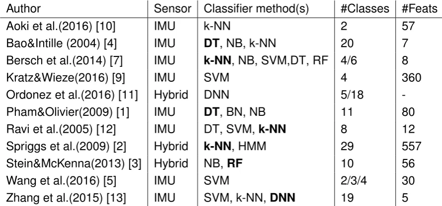
Author Sensor Classifier method(s) #Classes #Feats
Aoki et al.(2016) [10] IMU k-NN 2 57
Bao&Intille (2004) [4] IMU DT, NB, k-NN 20 7 Bersch et al.(2014) [7] IMU k-NN, NB, SVM,DT, RF 4/6 8
Kratz&Wieze(2016) [9] IMU SVM 4 360
Ordonez et al.(2016) [11] Hybrid DNN 5/18
-Pham&Olivier(2009) [1] IMU DT, BN, NB 11 80
Ravi et al.(2005) [12] IMU DT, SVM,k-NN 8 12
Spriggs et al.(2009) [2] Hybrid k-NN, HMM 29 557
Stein&McKenna(2013) [3] Hybrid NB,RF 10 56
Wang et al.(2016) [5] IMU SVM 2/3/4 30
[image:29.595.93.538.86.294.2]Zhang et al.(2015) [13] IMU SVM, k-NN,DNN 19 5
Table 2.3: Comparison of classifier method(s) used in existing studies for super-vised action segmentation and/or classification. ’IMU’ means here ei-ther an IMU or only accelerometer, ’Hybrid’ means a multi-modal model with both camera and IMU. The bold method gave the highest accuracy. ’#Classes’ means the number of classes. ’#Feats’ means the maximum number of features that is used for classification.
The deep belief network, which is a class of DNN, is used in [13]. They used MATLAB code from the homepage of Geoffrey Hinton [19].
2.3.4 Comparison
Classification methods used in action segmentation and/or recognition in different studies are compared in Table 2.3. The most popular methods are SVM and k-NN and very promising results are given by DNN, as shown in studies such as [13] and [11], who claims an improvement of 6% on average over non-deep architectures.
2.4 Evaluation
2.4.1 Introduction
All classification methods need evaluation afterwards to see how well the automatic annotation algorithm performed. Depending on the method, action segmentation and action recognition are evaluated separately.
2.4.2 Splitting data set
In order to properly test the classification model, it is necessary to split the data set in a training, validation and test set. The training set is used to train multiple models with different hyperparameters that are validated with the validation set. The best performing model is then tested on the test set to determine the performance. It is very important that the test set is not used during training and validation and that the model is not tuned anymore after testing, because then there is a risk of overfitting the model to the test set, which results in too optimistic results. Spriggs et al. [2] classify each frame from a withheld person’s sequence based on the grouping of the frames in the sequences of the remaining subjects. This is repeated in a cross-validation manner, withholding all people in turn and is called leave-one-out cross-validation (LOOCV). Aoki et al. [10] use LOOCV as well to evaluate their automatic segmentation results.
Another method that is used by, for example Bao&Intille [4] and Ravi et al. [12] is a user-specific approach where part of the data of one subject was used for training of one model and tested on the rest of the data for one subject. This was then repeated for all subjects and compared to LOOCV. Bao&Intille claim that, for their data set, the recognition accuracy was significantly higher for all algorithms under LOOCV than with the user-specific approach.
2.4.3 Evaluation measure
A frequently used measure to evaluate the performance of a classier is the accuracy. This is simply the number of correctly classified samples divided by the total number of samples.
However, the training data set can be highly unbalanced, because the activity can consist of mainly one action, for example, in Spriggs et al. [2], 25% of the frames was labeled as ’stirring’, while there were 29 actions defined. Therefore, in the case of action recognition, the overall classification accuracy is not an appropriate measure of performance when the action classes are highly unbalanced. Ordonez et al. [11] show that a trivial classifier that predicted every instance as the majority class could achieve very high accuracy, so they use the F-measure(F1) instead, a measure that considers the correct classification of each class equally important. It is the harmonic mean of the precision and recall for each of the classes, where precision is defined as T P
T P+F P and recall as T P
T P+F N, where T P, F P are the number
of true and false positives, respectively, andF N corresponds to the number of false negatives. The F-measure is then calculated as in Equation 2.14.
F1=
X
i
2∗wi
precisioni∗recalli
whereiis the class index andwi=ni/N is the proportion of samples of classi, with ni being the number of samples of the i-th class and N being the total number of samples.
Data set
The data from the experiment ’Quantified customer’ at TNO was used. This data set consists of the following data:
• EEG: biosemi
• Heart rate: mio fuse;
• ECG: biosemi;
• video: three camera’s. From the top, side and in front of the participant;
• IMU: 3 Shimmers, on each wrist and one on the hips
The experiment was done with 89 participants, recorded in three sessions: a ’dry cooking’ session where participants ’cooked’ with pieces of paper, then a session where subjects cooked a curry and then another ’dry cooking’ session. The real cooking session took almost twice as long as the dry cooking session.
We used the IMU data primarily and the video data for labeling, if necessary. The data set also includes event markers for each session, indicating the start of the audio instructions that the participants received during the experiment.
The raw IMU data dt contains the 3-axis accelerometer and 3-axis gyroscope data for time t, as shown in Equation 3.1
dt=[ax,ay,az,gx,gy,gz]t (3.1)
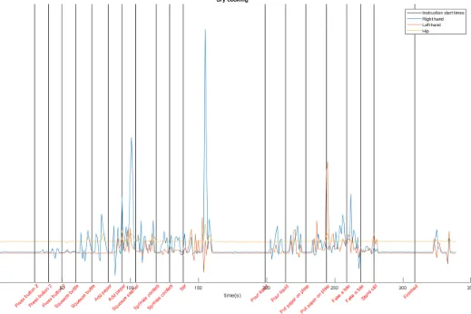
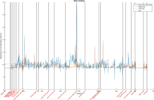
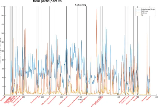
To give an indication how the data looks like, the magnitude of the signal vector over time (see Equation 2.5), for each of the three shimmers, of both the accelerom-eter and gyroscope data is given in Figure 3.1, Figure 3.2, Figure 3.3 and Figure 3.4 for the dry cooking and real cooking sessions. The times where the instructions are given to the participant are marked in the graph by the vertical lines. For the dry cooking sessions it is clearly visible that most of the action takes place between these instructions.
3.1 Data quality
Several subjects had data sets where the markers (which were used to synchronize the data with other data, such as the video and instruction start times) were missing. This meant only the data from 80 out of 89 subjects were in our data set.
From these 80 subjects, we assessed the quality of the data from each shimmer for each subject with a number 1 (bad quality) or 2 (partially bad quality) or 3 (good quality). Data was assessed as (partially) bad quality when one or more shimmers were not calibrated or properly connected, this led to almost useless data. However, 75% of the shimmer data was of good quality (rating 3), 18% of partially bad quality (rating 2) and only 7% of bad quality (rating 1).
The data of a subject was only used when the quality of the right-hand shimmer (which was the most important shimmer, because all participants were right-handed) was of good quality and the quality of data from the shimmers on the left hand and hip at least quaility 2. This meant that the data from 61 out 80 subjects was used.
Rating Shimmer 1 (RH) Shimmer 2 (LH) Shimmer 3 (hip) Total
3 (good) 69 (81%) 55 (65%) 68 (80%) 75%
2 (partially bad) 12 (14%) 26 (31%) 7 (8%) 18%
1 (bad) 4 (5%) 4 (5%) 10 (12%) 7%
Methodology
4.1 Approach
As described in subsection 2.3.1, there are several approaches we could take in order to automatically annotate IMU data. We did not take the approach where the data is segmented first and then action recognition is performed, because, in our data, it is very difficult to select a ground truth of (non) segment windows for training a classifier that could recognize segment windows.
Instead, we chose an approach where each window is classified as one of the actions, which is something that works well with our selection method (see sub-section 4.3.1), because we can select data where we are sure certain actions are performed or not, so a ground truth is easier to obtain.
4.2 Data windowing
We chose a window size of 1 second without overlap, because this is small enough to detect the shorter actions like pressing a button, but big enough to perform a meaningful frequency analysis. It is a similar window size as used by Zhang et al. [13], who calculated the same features for their model.
For every window, we calculated the n features over the shimmer data of that window ( n is different for different tasks: n=1 for the two class model and n=16 for the multi-class models, see section 4.9). These features were concatenated with the n features from the other two shimmers. Finally, these features from all three shimmers for the current window were concatenated with the features from the neighboring windows, creating9n features per window.
4.3 Ground truth
For classification we need a data set that is labeled, both for training the data and for validating the predictions. Most experiments that have a naturalistic setting use manual annotation from video, as described in subsection 2.2.2. However, because this is a time-consuming task and therefore not an option for most envisioned re-search projects, we examined other options:
1. Estimate the label for each of the windows of the data set, using all time-related information that is available, such as the start times for the auditory instructions, the length of the instruction and the average time that participants need for a certain action. This means that we have labels that should match the behavior for most participants, most of the time, though there is still uncertainty about the performance of the labels as ground truth, since participants are behaving rather freely and can for instance stand still in between stirring;
2. Use only dry cooking data for training. Here we know better what actions participants are performing and we could use this information for labeling the data. However, it is uncertain how well we can generalize this model to real cooking data. For instance, if a subject is adding something in a real cooking session, he will immediately start stir-frying the ingredient, while in the dry-cooking session, this can be performed as a separate action, which results in different motion data;
3. Select periods of time in the data set where we are very sure what action all participants are performing. It could be even necessary for dry cooking data to do this selection, as there are parts in the dry cooking data were we are unsure about. For instance, while participants may differ in the time that they need to empty a bowl of ingredients, we can be quite sure that they are all working on that for 5 seconds after the instruction;
4. For evaluation only: make a plot with the time on the x-axis and on the y-axis the prediction score (that is, the probability according to the model that the window belongs to a certain class). Mark on the x-axis the start times of the auditory instructions.
that there should be an increased probability for ’stirring’ during this period and we should be able to visually check this in such a graph.
We decided to make a selection of ground truth data in both the dry cooking and the real cooking data set, as described in option 3. We expect that the selection for dry cooking data is more accurate than the selection for real cooking data, be-cause the dry cooking session was more structured, so the performed actions are more predictable. Also, if it proves successful, this would support using a structured calibration set on real-life action.
We made a selection for the real cooking data as well, primarily to have a mea-surable indication of the performance of the trained model. Secondly, we used this selection for the training of a model that we compared to a model trained on dry cooking.
Finally we used a plot, as described in option 4, for a good indication of the performance of the trained model on all of the real cooking data. This is not an absolute metric, but gives an impression of the performance, especially for the non-selected parts (which are not evaluated otherwise).
4.3.1 Selection
For most actions that were performed during the cooking process, a selection is made for both the dry cooking session and the real cooking session. The actions that have selected data are:
• Standing still;
• Stirring;
• Pouring;
• Pressing button;
• Adding bowl;
• Squeezing bottle.
In Appendix A is described in detail how the selection is made and where the choices for this selection are based on.
4.4 Classification tasks
abstract action. This is also done because we wanted to start by evaluating the performance of our classifier on a simpler task and then compare it with the perfor-mance on more difficult tasks, with more classes. The combined abstract actions are as follows:
• Action: all selected actions that are not ’standing still’. At the time of running these tests, not all selections were made, so only ’stirring and ’pouring’ were used to train ’action’;
• Adding: this is the selections for ’adding bowl’, ’pouring’ and ’squeezing bottle’ combined.
From these (combined) actions, we defined the following tasks to see how the clas-sifier would perform:
• Two classes: ’standing still’ and ’action’;
• Three classes: ’standing still’, ’stirring’, ’pressing button’;
• Four classes: ’standing still’, ’stirring’, ’adding’, ’pressing button’;
4.5 Splitting train, validation and test set
As described in subsection 2.4.2, it is important to properly split the data set in a train and test set and train only on the train set in order to prevent overfitting. We chose to split only the real cooking data set separately in a train and test set with 80% of the participants as train set and other 20% for testing. The same participants were used on each run as train participants.
For validation, we used LOOCV on the train set. Each validation round, the data from another participant was taken as the validation set.
For the runs where the model trained on dry cooking data was run on real cooking data, the data was not split any more in a train and test set.
4.6 Tests
• Train on all selected dry cooking data, and validate using LOOCV;
• Run the model that is trained on all selected dry cooking data on all selected real cooking data .
• Run the four classes model trained on all selected dry cooking data on all real cooking data (also the non-selected parts) to get prediction scores of each of the four classes for each window;
• Train and validate on 80% of the selected real cooking data and test on the other 20%.
• Train and test on all selected real cooking data, using LOOCV. The four classes model is run on all real cooking data (also the non-selected parts) to get prediction scores of each of the four classes for each window;
4.7 Evaluation
We will use the following metrics for evaluation of the performance of the classifiers:
• Confusion matrix: this includes the overall accuracy and the recall and preci-sion for each class; This will be reported for all runs on selected data;
• score: From the recall and precision of each class we can calculate an F-score per class. We chose to report the average of the F-F-score for each class, which is described by Sokolova&Lapalme [20] as the macro-average. We also report an average of the F-score over only the action classes for runs with more than two classes, because this will show how well the classifier can dif-ferentiate between the different actions. This will be reported for all runs on selected data;
• A plot with prediction score over time, which can be visually evaluated in a plot, as described in section 4.3. This will be made for the runs with the four classes model on all real cooking data, where no ground truth is available, but still something can be said about the performance.
4.8 Classification method
these 5 neighbors that has a certain class to use as prediction score. This predic-tion score is used for evaluapredic-tion: it is plot over time to visually check how well the classification model performs on the real cooking data, as described in section 4.3.
4.9 Features
As described in subsection 2.2.3, there are many features that can be extracted for action recognition.
For the task of classifying only ’standing still’ and ’action’, we chose to use the magnitude of angular velocity (gyroscope data), following Aoki et al. [10]. Even though they use it for segmentation, our task is similar, as segmentation windows also include the windows where the participants are standing still and they also use this with k-NN.
For the other tasks of multi-class action recognition, we will follow Zhang et al. [13], who have very high performance on an action recognition task with these features on k-NN. This means we will use:
• mean (for each axis);
• STD (for each axis);
• the magnitude of acceleration (over all axes);
• frequency-domain energy (for each axis);
• frequency-domain entropy (for each axis);
• correlation of acceleration data between pairs of axes
for a total of 16 features per shimmer.
4.10 Balancing train set
As certain classes may be over-represented and others under-represented, there is unbalance in the training set. Since k is chosen to be 5 and not 1, the performance of k-NN could be influenced a little bit by the unbalanced classes (because for edge cases, where samples lie in between multiple classes, the class with more samples will tend to have the majority among 5 neighbors), therefore we tried balancing the train set.
Results
5.1 Two classes: Standing still and action
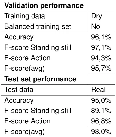
The results for the first classifier are shown here, a classifier with only the classes ’Standing still’ and ’Action’. The validation run results for the selected dry cooking set and the test results of this trained model on the selected real cooking set are shown in Table 5.1 for all participants. Figure 5.1 gives an indication of the performance by showing the predictions for participant 35.
Validation performance
Training data Dry
Balanced training set No
Accuracy 96,1%
F-score Standing still 97,1%
F-score Action 94,3%
F-score(avg) 95,7%
Test set performance
Test data Real
Accuracy 95,0%
F-score Standing still 89,1%
F-score Action 96,8%
[image:45.595.92.285.468.696.2]F-score(avg) 93,0%
Table 5.1: Classification results for the two classes model. F-score(avg) is the aver-age F-score over all classes.
Figure 5.1: Two class performance for participant 35 on selected real cooking data for the model trained on selected dry cooking data. Blue is standing still, orange is action. White is a non-selected part. 97.5% of the windows was predicted correctly, with an average F-score of 96.5%.
5.2 Three classes: Standing still, stirring and
press-ing button
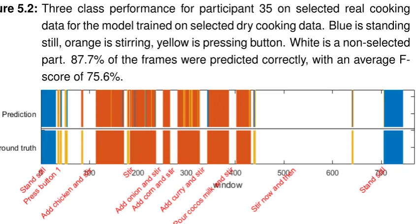
[image:46.595.87.510.516.744.2]The results for the second type of classifier are shown here, with the classes ’Stand-ing still’, ’Stirr’Stand-ing’ and ’Press’Stand-ing button’. For all participants, the validation and test results are shown in Table 5.2. An indication of the performance of the classifier on the selected parts is given for one participants with a higher performance (Figure 5.2 and one with a lower performance( Figure 5.3). Confusion matrices of the runs on dry cooking and on real cooking data are given in Figure 5.4 and Figure 5.5.
Figure 5.3: Three class performance for participant 71 on selected real cooking data for the model trained on selected dry cooking data. Blue is standing still, orange is stirring, yellow is pressing button. White is a non-selected part. 77.0% of the frames were predicted correctly, with an average F-score of 64.2%.
[image:47.595.177.436.474.746.2]Validation performance
Training set Dry Dry Real (80%) Real (80%)
Balanced No Yes, subsampled No Yes, subsampled
Accuracy 90,5% 88,8% 87,9% 76,8%
F-score Standing still 94,5% 93,2% 87,7% 85,6%
F-score Stirring 87,3% 87,2% 93,7% 84,9%
F-score Pressing button 75,9% 73,3% 43,5% 37,9%
F-score(avg) 86% 84,6% 75,0% 69,5%
F-score(action) 82% 80,2% 68,6% 61,4%
Test set performance
Test set Real Real Real(20%) Real(20%)
Accuracy 81,3% 83,8% 84,8% 71,5%
F-score Standing still 81,8% 88,3% 82,6% 83,4%
F-score Stirring 88,1% 90,1% 91,6% 80,1%
F-score Pressing button 40,9% 42,9% 42,5% 34,1%
F-score(avg) 70,3% 73,2% 72,2% 65,8%
[image:48.595.65.534.207.502.2]F-score(action) 64% 66,5% 67,1% 57,1%
5.3 Four classes: Standing still, stirring, adding and
pressing button
5.3.1 Selected data
[image:50.595.84.510.458.618.2]The results for the third type of classifier are shown here, with the classes ’Standing still’, ’Stirring’, ’Adding’ and ’Pressing button’. An indication of the performance of the classifier on the selected parts of both a participant with a higher and one with a lower performance is given in Figure 5.6 and Figure 5.7 for the unbalanced training set and in Figure 5.8 and Figure 5.9 for the balanced training set. For all participants, the validation and test results are shown in Table 5.3. Confusion matrices of the runs on dry cooking and on real cooking data are given in Figure 5.10 and Figure 5.11. These are included here to give an idea of the size of the data sets and to show the unbalance in the number of samples between classes, but also to show which classes are confused often.
Figure 5.7: Four class performance for participant 71 on selected real cooking data for the model trained on selected dry cooking data. Blue is standing still, orange is stirring, yellow is adding and purple is pressing button. White is a non-selected part. 52,7% of the frames were predicted correctly, with an average F-score of 49.0%.
[image:51.595.105.541.526.717.2]Figure 5.9: Four class performance for participant 71 on selected real cooking data for the model trained on balanced selected dry cooking data. Blue is standing still, orange is stirring, yellow is adding and purple is press-ing button. White is a non-selected part. 62.3% of the frames were predicted correctly, with an average F-score of 51.9%.
[image:52.595.149.409.474.747.2]Run # 1 2 3 4 5 Validation performance
Training data Dry Real (80%) Real (80%) Dry Dry
Balanced No No Subsampled Subsampled Over-sampled
Accuracy 79,4% 81,0% 73,1% 77,9% 77,7%
F-score Standing still 91,9% 91,1% 90,3% 93,1% 92,7%
F-score Stirring 53,8% 87,8% 80,8% 55,8% 55,1%
F-score Adding 74,8% 31,9% 43,1% 69,9% 71,2%
F-score Pressing button 61,7% 47,7% 45,7% 64,0% 61,1%
F-score(avg) 70,6% 64,7% 65,0% 70,7% 70,0%
F-score(action) 63,4% 55,8% 56,5% 63,2% 62,5%
Test set performance
Test set Real Real(20%) Real(20%) Real Real
Accuracy 58,0% 77,8% 69,5% 69,8% 67,4%
F-score Standing still 85,0% 86,3% 90,1% 88,4% 88,6%
F-score Stirring 63,6% 85,7% 77,0% 78,1% 75,4%
F-score Adding 31,4% 29,0% 40,5% 31,8% 32,7%
F-score Pressing button 38,3% 44,3% 41,5% 42,9% 41,0%
F-score(avg) 54,6% 61,3% 62,3% 60,3% 59,4%
[image:53.595.98.586.160.532.2]F-score(action) 44,5% 53,0% 53,0% 50,9% 49,7%
5.3.2 All data
[image:55.595.38.574.215.560.2]Several trained models were run on all data. However, we only report the prediction score of the different classes over time, as there is no (reliable) ground truth. These are shown in Figure 5.12 and Figure 5.13 for the models trained from run 1 and 4 in Table 5.3.
Discussion
6.1 ’Action’ versus ’standing still’
6.1.1 Classification performance
Our first objective was to see how well a classifier could differentiate between win-dows where the subject is standing still and where he or she is performing an action. From the results (Table 5.1), we can conclude that this is a simple task for our clas-sifier when the ground truth is clear, as we achieved an accuracy of 96.1% and an average F-score of 95.7% for the validation run, while the base line with two classes is 50%. Note that part of the inaccuracies are probably not real inaccuracies, but can be explained by some wrong labels in the ground truth of either the training set or the test set, as it is very likely that several participants were actually standing still during periods of expected action.
While we chose here for an approach that does not require annotation of the video data, it is clear that the most thorough test, which also tests and solves this issue, requires manual annotation.
6.1.2 Generalization dry to real
As can be seen in the comparison made in Figure 6.1, there was only a small dif-ference of -1.1% in accuracy and -2.7% in F-score between the validation run and the run on the real cooking data. This means that for training a model for detecting action, the training data does not have to be very similar to the test data. Most of the difference in performance is explained by the fact that it is easier to select data for dry cooking data, because participants are acting more according to instructions only.
Figure 6.1: Comparison in performance between different runs. No big differences are seen when the model is run on real cooking data.
6.2 Multiple classes
6.2.1 Classification performance
Secondly, we wanted to examine the performance of a classifier for multiple classes. This classifier should be able to differentiate between the different actions that are performed.
Three classes
From the results of the first of these tests, with three classes (Table 5.2), we can conclude that the classifier is able to perform well when trained and tested on dry cooking data, with an accuracy of 90.5% and an F-score of 86%, while the base line is 33%. Even the average F-score of the action classes is high, with 82%.
Training and testing with real cooking data shows a lower performance. Even though it has a test set performance of 84.8% accuracy and an average F-score of 72.2%, when we look at the individual F-scores, we see a low score for the class ’pressing button’, much lower than for dry cooking.
There are multiple explanations why ’pressing button’ has a low F-score, which are more or less likely:
ac-tions more at their own pace, so participants are more likely to perform other actions, like stirring, which can also be seen at the video. Therefore, this is a likely explanation for the lower F-score for ’pressing button’;
• The ground truth selection in the real cooking data (the test set) for other classes than ’pressing button’ contains windows where participants are press-ing a button. However, participants were not presspress-ing a button when not havpress-ing the instruction to do so. This is also the case with ’adding’, but not with ’stirring’ in the pan, which was done more spontaneously by participants. This means that it is not a likely explanation for the lower F-score for ’pressing button’;
• The real cooking session is more realistic and therefore the actions are more difficult to recognize, e.g. the participant is pressing a button with one hand, while stirring with the other. This particular behavior is seen on video and is therefore another likely explanation why ’pressing button’ has a lower F-score. In addition, this could explain inaccuracies in the classification of other actions as well.
’Pressing button’ is also a minority class in the real cooking data set (see Fig-ure 5.5), which means that it could be more difficult for the classifier to achieve a high performance.
For our application, automatic annotation of actions in the data, it depends on the specific question whether it is important to have a high performance on the minority classes. For some questions it is important need to know when these small actions are performed, for others, one mainly wants to know about the actions that are performed most.
We tried to improve the performance of the dry-dry and real-real runs on the minority classes by balancing the training set. As can be seen in Figure 6.2, this was not successful, as the average F-score on the actions went down for both dry cooking and real cooking. This is probably because the data amount is lower, as we deleted samples in the over-represented classes and because the model could not capitalize on differences in frequency of occurrence.
Four classes
Balancing the training set made the performance worse for both sets, similar to the three class model. Therefore we also tried balancing by over-sampling the under-represented class, but this performed even worse.
Figure 6.2: Comparison in performance between different runs of three classes models.
6.2.2 Generalization dry to real
Selected data
The runs where the dry cooking data was used as training set and the real cooking data as test set performed worse than the runs where only real cooking data was used (see Figure 6.2 and Figure 6.3), but still far beyond the base line of 25% for both the three and the four class model.
However, balancing the dry cooking training set improves the performance on the real cooking set significantly, especially for the action classes. This model is nearly as good as the model trained on real cooking data. The difference in the average F-score for the action classes between dry on real and real on real is only +0.6% in the case of three classes and +2.1% in the case of four classes.
Figure 6.3: Comparison in performance between different runs of four classes mod-els.
All real cooking data
When visually looking at the performance of the dry cooking model on the real cook-ing data in Figure 5.12, it becomes clear that for the selected parts, the model trained on dry cooking data is right, most of the time on average, however, it is confusing stirring and adding a lot. Balancing the training set gave much higher prediction score for stirring overall, but this score dropped when the participants were adding something, which makes sense, as participants were probably stirring most of the time and were not as much time busy with adding, which was predicted much more highly by the unbalanced model.
This is, however, an average over all participants, so it is difficult to say something about the specific performances per participant. Therefore the standard deviation is given as well. This shows that for example ’standing still’ is very similar for all participants. Other parts have a much higher standard deviation.
Conclusion and recommendations
7.1 Conclusion
In conclusion, we can say that, for up to four classes, we can automatically anno-tate the different actions pretty well, with the highest average F-score on the action classes of 53.0%. Especially classifying action and standing still has a very high performance, with an F-score of 95.7%. For classifying between three different ac-tions, the highest average F-score on the actions we achieved for real cooking data was 67.1% by the model trained on real cooking data.
However, even when using the data from a separate dry cooking session for training a four class model, we achieved an F-score on the actions of 50.9% and for training a three class model, an F-score of 66.5%. This means that training data from a structured session is almost as good for training a classifier that used in real cooking session, as training data from a more realistic session.
When taking an approach where data is first trained in a session like our dry cooking session, a balanced training set gave the highest performance.
Looking at the prediction score graphs (Figure 5.12 and Figure 5.13), we can conclude that the performance on real cooking data is good on average. While clearly manual annotation provides the best ground truth for training and evaluating models, this is often not possible due to research budget constraints. This study presented a way to evaluate different action recognition models without requiring manual annotation of videos.
7.2 Improving the performance of the models
There is definitely improvement in both training and evaluation by manually annotat-ing video and improvannotat-ing ground truth. However, this is somethannotat-ing we were lookannotat-ing to circumvent in this study, which worked moderately well.