Mapping electron tunnelling in a nanoparticle network to a cellular neural network

Nanoelectronics group

Mapping electron tunnelling in a

nanoparticle network to a cellular

neural network

University of Twente

Author: D.S. de Bruijn

26-10-2015

1

Table of Contents

Chapter 1: Introduction ... 3

Chapter 2: Theory ... 4

2.1 Single-electron tunnelling (SET) ... 4

2.1.1 Basic concept ... 4

2.1.2 Orthodox theory ... 5

2.1.3 Coulomb blockade and stability plots ... 6

2.1.4 Capacitance and voltage matrices ... 8

2.1.5 Energy levels ... 8

2.2 SIMON: a Monte Carlo SET simulator ... 9

Chapter 3: Adaptation to a cellular neural network (CNN) ... 11

3.1 Characteristics of CNNs ... 11

3.2 Equivalence between single-electron tunnelling and CNN dynamics ... 12

3.3 Current relation ... 13

3.4 Translation to Mathematica code ... 13

3.4.1 Adaptation of the one nanoparticle network ... 14

3.4.2 Adaptation of the two nanoparticle network ... 16

Chapter 4: Implementation & Method ... 17

4.1 A single nanoparticle simulation ... 17

4.1.1 Coulomb staircase and Coulomb oscillations ... 17

4.1.2 Stability plot... 17

4.2 Two nanoparticles simulation ... 18

4.2.1 Energy levels ... 18

4.2.2 Current... 19

Chapter 5: Results & discussion ... 20

5.1 Results single nanoparticle simulation ... 20

5.1.1 Coulomb staircase and Coulomb oscillations ... 20

5.1.2 Stability plot... 21

5.2 Results multiple nanoparticles simulation ... 23

5.2.1 Energy levels ... 23

5.2.2 Current... 24

Chapter 6: Conclusion & recommendations ... 25

6.1 Conclusion ... 25

2

Acknowledgement ... 26

References ... 27

Appendix A: Mathematica script of one nanoparticle network ... 28

Appendix B: Mathematica script of a two nanoparticle network ... 31

3

Chapter 1: Introduction

Today's scientists are looking for new ways to do computations faster, more efficiently and to master more complex computations like pattern recognition. Especially pattern recognition is for conventional computers a very difficult and a time consuming task. To improve upon doing these sorts of computations new concepts must be developed.

An example of such a new concept is for instance the recent work of S.K. Bose and C.P. Lawrence, in which a designless nanoparticle network is turned into reconfigurable Boolean logic by evolution[1]. These networks of interconnected metal nanoparticles act as strongly nonlinear single-electron transistors[2], [3] and can be turned into any Boolean logical gate. This concept is very interesting for further research to see if more advanced tasks like pattern recognition can be handled.

Looking into the behaviour of these networks before fabricating them requires an appropriate computer model. At this moment circuits built of single-electrons can be modelled by a simulator for single-electron tunnel devices and circuits called SIMON 2.0 [4],[5]. However, SIMON is only suitable for simulating small amounts of nanoparticles, because for large systems the computation time becomes too large, due to the use of Monte Carlo simulations [3]. Therefore, another model must be found to simulate the behaviour of larger systems.

In this report will be investigated if it is possible to map a nanoparticle network to a cellular neural network (CNN) and discover the behaviour of such networks. The advantages of CNNs are [6],[7]:

 Scalability

 High-speed parallel signal processing

 Local dynamics, local feedback and local feedforward

To check if the adopted CNN model is valid, the results of the CNN model will be compared with the results of SIMON which is proven to be realistic for small networks. Later on, if the CNN model matches with SIMON, the model can be tested for bigger networks. The CNN model will be made in Wolfram Mathematica [8].

4

Chapter 2: Theory

The basics of single-electron tunnelling (SET) will be discussed in this subsection. First the basic concept of SET will be explained. Secondly the simplified theory used to describe SET will be introduced. Then the special behaviour of SET will be discussed, further more the voltage relations in a basic network and energy levels are explained. Finally, the working principle of the simulation software SIMON is presented.

2.1 Single-electron tunnelling (SET)

2.1.1 Basic concept

First of all, a conducting island or nanoparticle is needed for SET. At the right conditions, which will be introduced next, SET has a very interesting behaviour. Under these conditions the tunnelling of individual electrons can be controlled. The tunnelling rate can for example be influenced by a bias voltage at the nanoparticle.

The tunnelling will now be discussed in more detail. Lets first assume that the island has the same amount of electrons as it has protons, such that the island is electroneutral as can been seen in figure 1. A weak external force may add an extra electron from the outside to the island. Now the island is negatively charged and will repel electrons from the outside by its electric field E.

figure 1: At the left of the arrow an electroneutral island is depicted. One single electron is added to this island, due to a weak external force from outside. The result is shown on the right: a negatively charged island, which generates an

electric field which repels other electrons.

However, in general the energy that is needed to add an electron to the island is not expressed as the strength of the electric field but as the charging energy as can be seen in equation ( 1 ). When one electron is added, the electrostatic potential changes by the charging energy. This charging energy is inversely proportional to the capacitance of the island, which is again related to the size of the island by C = εS/(4 d) [9]. So, the smaller the nanoparticle, the higher the charging energy.

( 1 )

( 2 )

( 3 )

The charging energy is not the only energy contribution in this system. The electron addition energy

5 2.1.2 Orthodox theory

Single-electron tunnelling can be described by different theories with each there pro's and con's. In this paper the 'Orthodox theory' [10] will be explained, since the CNN model will be based on this model. The Orthodox theory is a simple but very effective method in describing the physical behaviour of single electrons. It translates the quantization of charge into the quantization of a continuous spectrum of energy states.

The Orthodox theory makes the following major assumptions [2]:

1. The electron energy spectrum is considered continuous. This will give an adequate observation as long as Ek << EC.

2. The tunnel time of an electron is negligibly small in comparison with other time scales, which is valid for tunnel barriers in single-electron devices.

3. Multiple tunnelling processes at the same time by a single electron called "cotunnelling" are neglected. This assumptions holds if the resistance R of all the tunnel barriers is much higher than the quantum resistance RQ. RQ is typically 6.5 kΩ [2].

The Orthodox theory manages to be in quantitative agreement with nearly all experimental data for systems with metal conductors. For semiconductor structures the theory gives qualitatively description of most obtained results. The networks in this research are based on metal conductors and will therefore give quantitative results based on the Orthodox theory.

Now the tunnel rate Γ will be introduced. The tunnel rate is the number of electrons that tunnel through a barrier per second. It depends on the reduction ΔW of the free (electrostatic) energy in the total system due to the tunnelling event as is shown in equation ( 4 ). One can observe from this equation that the tunnel rate is linear dependent on the change of free energy at 0K. The free energy depends on voltage drop across the barrier before Vi and after Vf a tunnel event as stated by equation ( 5 ).

( 4 )

_{( 5 )}

The calculations seems to be straight forward, but problems can already occur in basic circuits when multiple tunnelling events are possible on the same time. All possible states of the network have to be integrated into a system of master equations ( 6 ), which describes the change of probability in time for each state. The master equation will blow up when a multidimensional space is considered with all its possible states. A way to solve these complex systems is with the Monte Carlo Method which will be discussed in section 2.2 SIMON: a Monte Carlo SET simulator on page 9. [11] In this report the master equations will be mapped to a CNN to check if it can solve complex systems as will be explained in Chapter 3: Adaptation to a cellular neural network (CNN).

6 The most significant effects that are neglected by the Orthodoxy theory are cotunnelling and discrete energy levels. Cotunnelling is negligible if the resistance R of the barriers is much higher than the quantum resistance RQ. The discrete energy levels start to play a role for very small islands. At that moment the quantum splitting Ek between electron energy levels may become larger than EC and kBT

as a result the energy dependence of the tunnelling rate changes. For large differences in energy the tunnel rate will reach a constant rate.

2.1.3 Coulomb blockade and stability plots

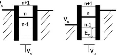
At low temperatures for small structures and under the right conditions the tunnelling behaviour of electrons at nanoparticles can be described by the Orthodox theory as mentioned before. In this section a look is taken at the special behaviour of SET. Due to the charging energy a single nanoparticle can be in two states as is shown in the double tunnel junction in figure 2. Once the potential outside a nanoparticle has overcome the charging energy an electron can tunnel to the nanoparticle. However, to establish a current it should also leave the nanoparticle through another barrier. If the electron cannot leave the nanoparticle and its trapped it is called a Coulomb blockade.

figure 2: Different states of conduction of a nanoparticle with energy level n. In the right network electrons can tunnel from and to the nanoparticle via energy level n, such that there is a current. At the left nanoparticle there is a so called

Coulomb blockade and no current will flow.

The effect of the Coulomb blockade in double tunnel junctions can be seen from the Coulomb staircase and Coulomb oscillations in figure 3. In the top figure Vb is the bias or source voltage. The so called Coulomb blockade is clearly visible at Vb = 0V, because the charging energy must first be overcome before a current can start to flow. The step like behaviour is due to new energy levels that are able to conduct with an increasing bias voltage.

7

figure 3: The top figure, a I-Vb curve, shows the Coulomb staircase. The bottom figure, a I-Vg curve, shows the Coulomb oscillations. The simulation is done at 0K and the capacitances of the barriers are 1aF. (Source [3])

Now it is time to analyse the behaviour of the complete double tunnel junction. This can be done by looking at the current of the nanoparticle while adjusting both the bias and the gate voltage. This results in a stability plot as is shown in figure 4. The diamond structures are well known as Coulomb diamonds. The grey areas indicate the stable areas and the white areas are instable. So, instable means that there is a current and the stable areas are the result of the Coulomb blockade without a current.

8 2.1.4 Capacitance and voltage matrices

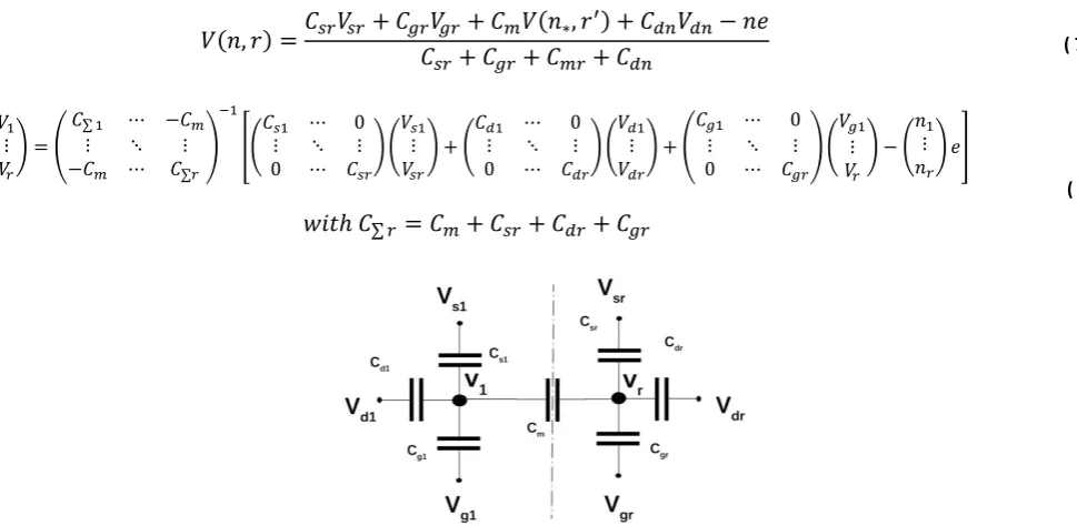
In order to find an expression for the tunnelling rate defined by the Orthodox theory the change in free energy of each tunnelling event must be calculated. To do this all the potentials and capacitances in the network must be known. The nanoparticles are interconnected by tunnel barriers which can be represented by a capacitance and resistance. Each individual nanoparticles can have a source, drain, bias and multiple neighbouring nanoparticles as is shown in figure 5. The potential

of nanoparticle r is expressed in equation ( 7 ). The voltage and capacitance matrices for a large network can be expressed as in equation ( 8 ). This equation is based on the circuit in figure 5 and the assumption that the charging energy is constant.

( 7 )

( 8 )

figure 5: This network shows all the voltages and capacitances within a nanoparticle network. Vr is the potential of

nanoparticle r, Vsris the source voltage, Vgr is the gate voltage and Vdr is the drain voltage of nanoparticle r.

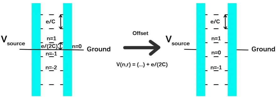
2.1.5 Energy levels

9

figure 6: At the left the energy levels of a nanoparticle without an offset. The source and gate voltage are 0V. In the right figure the offset is introduced.

In order the find out which highest occupied energy level is applicable for a certain nanoparticle a rule of thumb can be used. If and the network is considered as a simple RC network without a charging energy, can be calculated as is shown in equation ( 9 ). Considering the discrete energy levels near will give a good estimation of the relevant energy levels.

( 9 )

2.2 SIMON: a Monte Carlo SET simulator

A proven simulator for single-electrons tunnel devices is SIMON [4],[5]. SIMON is capable of simulating the random dynamics of complex systems. The working principle of SIMON will now be discussed.

The basic working principle of the Monte Carlo method can be seen in the flowchart of figure 7. At first all the tunnel rates, free energy changes and the duration to the next tunnel events of all the possible tunnelling events are calculated. This is done using the capacitance matrix of the network. When all the calculations are done, one single event with the smallest duration will take place and this process is then started over and over. One can imagine that this takes a lot of computations time for large networks, so the computation time mainly depends on the number of tunnel junctions and nodes in the network.

Despite the long computation time the Monte Carlo method has the following advantages [5]:

1. It takes underlying microscopic physics into account for a better transient and dynamic characteristics of SET circuits.

10

11

Chapter 3: Adaptation to a cellular neural network (CNN)

In this chapter the adaptation to a cellular neural network will be discussed by first looking at the characteristics of CNNs. Secondly the equivalence between single-electron tunnelling and CNN dynamics is explained. After this the current in the network is expressed. Finally the adaptation to SIMON and the CNN model in Mathematica is explained for an one and two nanoparticle network.

3.1 Characteristics of CNNs

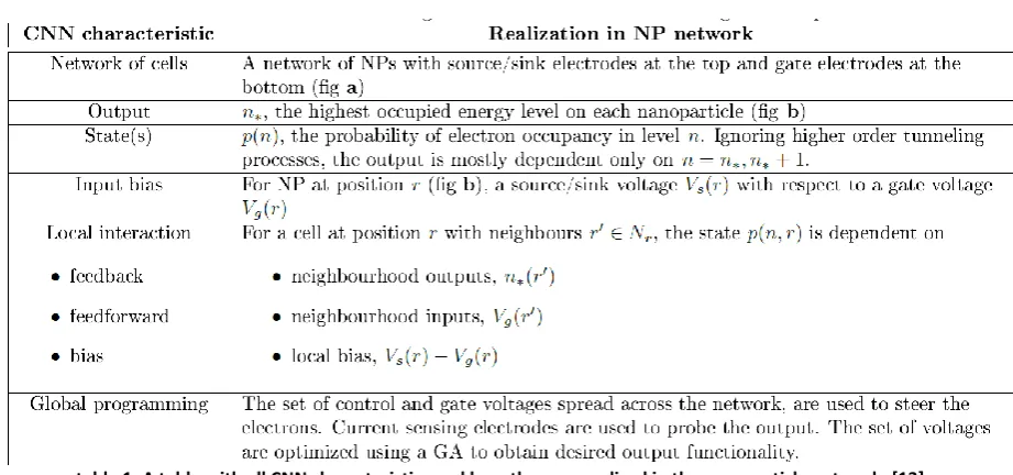
To be able to adapt a network of nanoparticles to a CNN the characteristics of such a CNN must be determined. In this report the list below shows the characteristics of the CNN as described by T. Roska and L. Chua [12]. A CNN is,

1. a network of nonlinear cells

2. where each cell has an output corresponding to its state 3. which is determined by its own input bias plus...

4. local interactions by feedback and feedforward mechanisms

5. that is measured and controlled by global lines (which maybe sparse)

In figure 8 the mapping of a nanoparticle network to a CNN is visible. All the characteristics of the list above are taken into account. In table 1 the realization in a nanoparticle network is explained more elaborate.

figure 8: a) A schematic of a nanoparticle network. b) In this network electrons tunnel between neighbouring nanoparticles and source/sink electrodes as described by the master equation ( 10 ) introduced in the next section. c)

Simplifying the master equation satisfies the essential characteristics of a CNN as is explained in table 1. [13]

12

3.2 Equivalence between single-electron tunnelling and CNN dynamics

The following assumptions in this section are proposed by C.P. Lawrence.[13] The master equation for single-electron transport in general is

( 10 )

where

 is the probability of an electron to be in energy level n at a nanoparticle located in position r

 is the rate for the tunnelling process from position r' to r, energy level n' to n

 n' iterates over all possible energy levels Z, r' iterates over all nanoparticles in neighbourhood Nr

To estimate a lower-bound for the dynamical complexity of this system, the equations are simplified by introducing many working assumptions:

 Neighbourhood tunnelling: electrons only tunnel from the highest occupied energy level  Source/sink tunnelling: electrons tunnel from or to the energy level -eVs with a tunnel rate

or





, gives the tunnelling rate as a function of

energy/voltage and a constant tunnel resistance. is a ramp function



gives the corresponding voltage potential by assuming a constant

charging energy

The simplified master equation thus becomes,

( 11 )

( 12 )

The master equation will be solved for stable systems, so such that the probability of an electron to be at nanoparticle r at energy level n is,

13

3.3 Current relation

In order to give expression to the current in a network one can look at the tunnelling rates of electrons leaving and entering a nanoparticle and the probabilities of electrons to be at a certain energy level. The probability times the tunnel rate gives the number of electrons per second that tunnel, which is current. In general a current can be expressed as,

( 14 )

The current in the two nanoparticle system can be described as is shown in equation ( 15 ). In figure 9 a graphical representation of the two nanoparticle network is shown.

( 15 )

figure 9: In this schematic two nanoparticles are drawn which interact with each other and with the source and sink indicated by the dashed vertical lines. All the possible currents between the source, sink and nanoparticles are IA, IBand

IC.

3.4 Translation to Mathematica code

In table 2 the mathematical descriptions of the CNN model are translated to the code in Mathematica. In Mathematica the symbol r' cannot be used and is replaced by the rr.

CNN model Mathematica model

14

table 2: Mapping of the CNN model to the code in Mathematica.

3.4.1 Adaptation of the one nanoparticle network

The first model will only consists of one nanoparticle to check if the fundamental behaviour of the nanoparticle can be described by the CNN model. The circuit used in SIMON can be seen in figure 10.

All the tunnel barriers will have a resistance of 10kΩ, the bias capacitance will be kept at 20aF and the temperature is set to 0K for all simulations. The source capacitance Cs and mutual capacitance Cm

can be changed depending on the goal of the simulation. Different capacitance values should give different shapes of Coulomb diamonds.

figure 10:One nanoparticle network in SIMON

The code used to describe a one nanoparticle network in Mathematica is shown in Appendix A:

15 simple, because the only unknown variable, is the energy level n of this one nanoparticle. The probability expressed in equation ( 13 ) can easily be calculated for each energy level. First of all the potentials are calculated using equation ( 8 ).Then the tunnel rates are calculated and finally the probability is expressed.

To make the calculations more efficient not all the energy levels should be considered when calculating the probability. It should be enough to consider only the relevant energy levels as explained in section 2.1.5 Energy levels. This is done by using the following line of code,

To define the relevant energy levels the energy levels close to the value in MatrixN should be found. This can be done using the following line of code to make a list of levels,

The probability gives information about the way an energy level is filled and this can be done in three states as mentioned below in table 3. The graphical representation of these states is shown in figure 11. Of course, only the occupied energy levels will have a current contribution in the network. Therefore, by checking for the relevant energy levels if one of them is sometimes occupied, one can determine if the network is stable or not. Only one occupied energy level is enough to have a current contribution and for the network to be instable.

State Probability

Always filled p(n,r) = 1

Sometimes occupied 0 < p(n,r) < 1

Always empty p(n,r) = 0

table 3: Three different possible states of an energy level with its probability.

figure 11: Different states of the energy level n

The pseudo code of the Mathematica script can be considered as follows:

 Initialise capacitance and voltage matrices  Calculate the potentials of all nodes  Approximate the relevant energy levels

 Calculate tunnelling rates to and from the nanoparticle for these energy levels  Calculate the probability of each energy level

 Evaluate the probabilities by checking if the configuration is stable or instable o An energy level is in the occupied state -> Instable

16 3.4.2 Adaptation of the two nanoparticle network

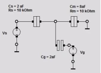
The next step is to look at a more complicated two nanoparticle network. An interesting network to look at is the network in figure 12, because the nanoparticles are placed in parallel and coupled which gives an interesting stability. This network is thoroughly examined by K.S. Makarenko in her book Charge Transport in Bottum-Up Inorganic-Organic and Quantum-Coherent Nanostructures [14]. The two nanoparticles are placed in parallel to the source and the drain as can be seen in figure 12. All the tunnel barriers will have a fixed resistance of 10kΩ and the temperature is set to 0K.

figure 12: Two particle network in SIMON inspired by the work of Ksenia S. Makarenko. [14]

The equivalent CNN model of the SIMON model introduced in the section above can be found in

Appendix B: Mathematica script of a two nanoparticle network on page 31.

The first step is to calculate all the voltages in the circuit. This time nanoparticle 1 and 2 interact with each other and both potentials are dependent on each other. As explained in section 2.1.4

Capacitance and voltage matrices the complete network can be described by capacitance and

voltage matrices. By doing this matrix calculation all the potentials in the network for any given combination of energy levels can be calculated by equation ( 8 ).

After this the energy levels can be expressed by taking care of the offset. This is done using the following lines of code,

17

Chapter 4: Implementation & Method

In this chapter the implementation and testing method of different networks is described. There will be started with a simple network of just one nanoparticle. A few basic examples from literature will be examined for this network like the well known Coulomb staircase and oscillations. After that a look is taken at the stability plot. Finally the current and stability of the two nanoparticle model will be considered.

4.1 A single nanoparticle simulation

4.1.1 Coulomb staircase and Coulomb oscillations

The first comparison between the CNN model and SIMON will be by comparing the Coulomb staircase and Coulomb oscillations of both models. The Coulomb staircase will be obtained by adjusting the voltage source from -1.0V to 1.0V and the bias voltage is fixed at 0V. In SIMON the current from the source to the nanoparticle is measured as can be seen in figure 13. In Mathematica the probability times the tunnel rate from and to the source will give the current. The source and mutual capacitance are set to 0aF in this simulation. The expected charging energy will be

. To compare the results of the CNN model in Mathematica and the results in SIMON the obtained data of both programs are converted to Excel and plot in one figure.

The next simulation will show the Coulomb oscillations by adjusting the gate voltage from -1.0V to 1.0V and fixing the source voltage at 0.05V. In SIMON the current from the source tot nanoparticle is measured as can be seen in figure 13. In Mathematica the probability times the tunnel rate from and to the source will give the current. The source and mutual capacitance are set to 0aF in this simulation. To compare the results of the CNN model in Mathematica and the results in SIMON the obtained data of both programs are converted to Excel and plot in one figure.

figure 13: Measuring circuit for Coulomb staircase and oscillations in SIMON.

4.1.2 Stability plot

Next the stability plot of the one nanoparticle circuit in figure 10 will be made. A stability plot shows normally the amount of activity for a certain configuration of the network. Activity means in that context the number of electrons per second that tunnel. However, later on in this report will be explained that the current cannot be calculated for multiple nanoparticle systems, therefore it is more convenient to check whether a system is stable (no current) or instable (any current).

The stability plot is obtained by varying Vgfrom -0.1V to 0.1V and Vs from -0.03V to 0.03V. To get a

18 the CNN model in Mathematica. This means that the activity at no conduction is 0 and set to 1 for any current. The model is tested for multiple configurations of the capacitances to see if the shapes keep matching. The first test is based on Cs=2aF, Cg=2af and Cm=8aF. The second test is done for Cs=Cg=Cm=2aF.

As described before in section 2.1.4 Capacitance and voltage matrices the algorithm estimates the appropriate energy levels for a combination of potentials. In this case a total range of four energy levels is considered. The estimation is correct if the diamonds will repeat themselves along the x-axis (gate voltage). The gate voltage will be changed from 3V to 3V, the source voltage is changed from -0.5V to -0.5V and the capacitances in this network are all 0.16aF.

4.2 Two nanoparticles simulation

4.2.1 Energy levels

To check if the energy levels are correctly calculated by the CNN model, the energy levels will be visually compared to the stability plot in SIMON. This stability plot is shown in figure 14. The energy levels will be compared by looking at the six different regimes indicated in the figure at Vs=3mV. Regime 1,3 and 5 should be stable and regime 2,4 and 6 should be instable.

After this the probability for each energy should be checked to see if this is implemented the right way.

19 4.2.2 Current

By evaluating numerically a random network one can easily check whether the current relation discussed in section 3.3 Current relation on page 13 holds and satisfies the expected behaviour. In this case one expects that the source current equals the sink current. To check this the random network in figure 15 will be examined. If the relation holds for this network one should investigate more situations and check whether this holds for all possible networks.

figure 15: A random network to check if the proposed current equations hold. From left to right are visible: the source, the first nanoparticle, the second nanoparticle and the sink. The source voltage is -4V, the sink voltage is 0V and the two

20

Chapter 5: Results & discussion

In this chapter the results of the simulations will be presented and discussed.

5.1 Results single nanoparticle simulation

5.1.1 Coulomb staircase and Coulomb oscillations

The results of the Coulomb staircase and Coulomb oscillations are respectively shown in figure 16 and figure 17. In the figure of the Coulomb staircase one can clearly see that the Coulomb blockades of both models match. There is no current from 0.46V to 0.54V, therefore the charging energy is 0.08V for this nanoparticle as expected. The slope of the current for the CNN model does not match with the slope of the current in SIMON. However, the slope could be adjusted by changing the ramp function as it is given in section 3.2 Equivalence between single-electron tunnelling and CNN dynamics on page 12.

The Coulomb oscillations of the CNN model and SIMON have the same period, but the amount of current is again not equal. In this case the solution can be changing the ramp function as well. There is also a small mismatch in the width of each peak.

figure 16: The Coulomb staircase of the nanoparticle network for the CNN model and SIMON is shown by plotting the current versus the source voltage. In this network Vg=0V. The left figure shows the complete plot and the right figure shows a zoom in of the Coulomb blockade. The current for the CNN model is expressed as the probability times the

tunnel rate from and to the source.

-2,75E-05 -2,25E-05 -1,75E-05 -1,25E-05 -7,50E-06 -2,50E-06 2,50E-06 7,50E-06 1,25E-05 1,75E-05

-0,50 0,00 0,50

Cu rr e n t (I)

Source voltage (V)

Coulomb staircase one NP

network

SIMON CNN model

-1,25E-06 -7,50E-07 -2,50E-07 2,50E-07 7,50E-07 1,25E-06

-0,10 -0,05 0,00 0,05 0,10

Cu rr e n t (I)

Source voltage (V)

Coulomb staircase one NP network

- zoom in

21

figure 17: The Coulomb oscillation of the one nanoparticle network for the CNN model and SIMON is shown by plotting the current versus the gate voltage. In this network Vs=0.05V. The current in Mathematica is expressed as the probability

times the tunnel rate from and to the source.

5.1.2 Stability plot

The stability plots of the one nanoparticle network are shown in figure 18 and figure 19. There is an exact match between the stability plots of the CNN model and SIMON. The values do also match with the values from literature in figure 4.

figure 18: The left figures correspond to the results of the CNN model and the results to the right correspond to results of SIMON. At the x-axis the gate voltage is shown and at the y-axis the source voltage. The capacitance values are Cs=20aF,

Cg=20af and Cm=80aF.

-5,00E-08 0,00E+00 5,00E-08 1,00E-07 1,50E-07 2,00E-07 2,50E-07

0,00 0,20 0,40 0,60 0,80 1,00

Cu

rr

e

n

t

(I)

Gate voltage (V)

Coulomb oscillations one NP network

SIMON

22

figure 19: The left figures correspond to the results of the CNN model and the results to the right correspond to results of SIMON. At the x-axis the gate voltage is shown and at the y-axis the source voltage. The capacitance values are

Cs=Cg=Cm=20aF.

In figure 20 it is clear that the Coulomb diamonds will repeat themselves along the x-axis as expected. This means that the approximation of finding the highest occupied energy level works and four energy levels is enough to simulate the behaviour of a one nanoparticle network.

23

5.2 Results multiple nanoparticles simulation

In this section the results of the two nanoparticle network will be presented and discussed.

5.2.1 Energy levels

The energy levels of the CNN model are plot in figure 21 for the six different regimes. One can visually check that regime 1,3 and 5 are indeed stable and regime 2,4 and 6 are instable. So, the energy levels are implemented the right way.

However, if a look is taken at the probabilities there is a mismatch. In figure 22 there is an example given of a wrong probability. If we look at the energy level (0,0) the number of electrons on both nanoparticles is 0. The second nanoparticle will give a probability of 1, because it is in between ground and the level (0,0) of nanoparticle 1. It does not know that level (0,0) of nanoparticle 1 will never be filled and gives therefore wrong information.

24

figure 22: Example of a wrongly expressed probability.

5.2.2 Current

The random network proposed in section 4.2.2 Current is numerically evaluated to check if the proposed current equations holds. The results of the equations are in equation ( 16 ). Despitefully the current IA does not equal the current in IC as expected, therefore the current cannot be derived from this CNN model. One can see that the total amount of current in the network is in balance. This is because for each individual nanoparticle the same amount of current that enters the nanoparticle leaves the nanoparticle, but there is no communication between the neighbours, so there can be a difference in current between two neighbours.

Another problem is the fact that only the highest occupied energy level of the neighbour is taken into account when looking at the tunnelling rates. Even if lower energy levels of neighbouring particles conduct, their current contribution is not taken into account.

25

Chapter 6: Conclusion & recommendations

6.1 Conclusion

To sum up, the goal of this research was to check if the adopted CNN model is valid by comparing it to simulations in SIMON. First of all one can conclude that the current in a nanoparticle network cannot be expressed using the CNN model. However, giving expression to the stability of a nanoparticle network seems more promising.

The stability of an one nanoparticle model can perfectly be simulated by the CNN model and matches with literature. A nice feature is that the simulation time is reduced by only calculating a minimum amount of relevant energy levels for a certain configuration of potentials.

So far, the stability of the two nanoparticle model cannot be simulated. The energy levels are in agreement with the expected levels, but the probability is wrong. The master equation is too much simplified and the tunnel rates of the neighbouring particles should be coupled.

The moment the two nanoparticle network shows accurate results the number of nanoparticles can easily be scaled up, since the two nanoparticle problem is written using only matrices, which are scalable to any size.

6.2 Recommendations

The tunnel rates of the neighbouring particles should be coupled, such that the probability can be expressed in the right way.

In the future it is good to integrate for multiple nanoparticle networks also the feature of calculating only the relevant energy levels instead of taking all levels into account. This will save a lot of

computation time and it will be easier to simulate stability plots of a higher resolution.

26

Acknowledgement

This bachelor thesis could not have successfully been finished without the generous help of a few people. These people took a lot of their valuable time and helped me to gain insight into the wonderful world of nanoparticles and helped to overcome the obstacles that I found on my way.

I would like to thank Celestine Lawrence and Wilfred van der Wielfor their advice and help as supervisors during this project. They were of great support and gave me new insights and introduced me to the right people to help me further.

27

References

[1] S. K. Bose, C. P. Lawrence, Z. Liu, K. S. Makarenko, R. M. J. van Damme, H. J. Broersma, and W. G. van der Wiel, “Evolution of a designless nanoparticle network into reconfigurable Boolean logic,” Nat. Nanotechnol., no. September, pp. 1–6, 2015.

[2] K. K. Likharev, “Single-electron devices and their applications,” Proc. IEEE, vol. 87, no. 4, pp. 606–632, 1999.

[3] C. Wasshuber, Computational Single-Electronics. Springer Wien New York, 2001.

[4] C. Wasshuber and H. Kosina, “A single-electron device and circuit simulator,” Superlattices

Microstruct., vol. 21, no. 1, pp. 37–42, 1997.

[5] C. Wasshuber, H. Kosina, and S. Selberherr, “SIMON - A simulator for single-electron tunnel devices and circuits,” IEEE Trans. Comput. Des. Integr. Circuits Syst., vol. 16, no. 9, pp. 937– 944, 1997.

[6] L. O. Chua and L. Yang, “Cellular neural networks: applications,” IEEE Trans. Circuits Syst., vol. 35, no. 10, pp. 1273–1290, 1988.

[7] L. O. Chua and L. Yang, “Cellular neural networks: theory,” IEEE Transactions on Circuits and

Systems, vol. 35, no. 10. pp. 1257–1272, 1988.

[8] “Wolfram Mathematica.” [Online]. Available: http://www.wolfram.com/mathematica/. [Accessed: 30-Sep-2015].

[9] L. L. Sohn, L. P. Kouwenhoven, and G. Schön, “Mesoscopic Electron Transport,” in Mesoscopic Electron Transport, 1997, p. 21.

[10] D. V. Averin and K. K. Likharev, “Single electronics: A correlated transfer of single electrons and Cooper pairs in systems of small tunnel junctions,” in Single electronics: A correlated transfer of single electrons and Cooper pairs in systems of small tunnel junctions, 1991, pp. 173–271.

[11] K. K. Likharev, N. S. Bakhalov, G. S. Kazacha, and S. I. Serdyukova, “Single-electrom tunnel junction array: an electrostatic analog of the Josephson transmission line,” IEEE Trans. Magn., vol. 25, no. 2, pp. 1436–1439, 1989.

[12] L. Chua and T. Roska, Cellular Neural Networks and Visual Computing: Foundations and

Applications. Cambridge University Press, 2005.

[13] “Private communication with C.P. Lawrence.”

[14] K. S. Makarenko, Charge Transport in Bottum-Up Inoarganic-Organic and Quantum-Coherent

Appendix A: Mathematica script of one nanoparticle

network

Constants

In[1]:= e = 1.60*10^-19;

R0 = 1*10^5;

Cg1=20*10^-19;

Cs1 =20*10^-19;

Cd1 =80*10^-19;

NUMlevels =1;

(* The total number of calculated energy levels is NUMlevels*2+2 *)

numneighb = 0;

(* Number of neighbours is equal to the number of particles -1 *)

Initialisation

In[8]:= vd1 = 0;

vs1= vs;

vg1= vg;

In[11]:= MatrixC = {Cs1+Cg1+Cd1};

MatrixCs = {Cs1};

MatrixCg = {Cg1};

MatrixCd = {Cd1};

(* Defines the capacitance matrices each row maps to a particle *)

MatrixVs := {vs1};

MatrixVg := {vg1};

MatrixVd := {vd1};

Matrixn := level[n1];

level[n_] := n-12;

(* Defines the voltage matrices each row maps to a particle *)

MatrixV :=1MatrixC*

(MatrixCs.MatrixVs+MatrixCg.MatrixVg+MatrixCd.MatrixVd-Matrixn*e);

MatrixN := 1

e (MatrixCs.MatrixVs+MatrixCg.MatrixVg+MatrixCd.MatrixVd);

(* Calculates all the node potentials and sets them in matrix v *)

MatrixR = {10^99};

MatrixRs = {R0};

MatrixRd = {R0};

(* Defines the resistance matrix,

not connected nodes have a very high resistance *)

In[25]:= Toneighbour[r_, rr_] := v[[r]] -v[[rr]]

e*MatrixR[[r]]

;

(* All tunnelling electrons from node r to neighbours *)

Tosource[r_]:= v[[r]] -MatrixVs[[r]]

e*MatrixRs[[r]] ;

Tosink[r_]:= v[[r]] -MatrixVd[[r]]

e*MatrixRd[[r]] ;

(* All tunnelling electrons from node r to source or drain *)

Fromneighbour[r_, rr_] := v[[rr]] -v[[r]]

e*_MatrixR[_r] ;

(* All tunnelling electrons from neighbours to node r *)

Fromsource[r_]:= MatrixVs[[r]] -v[[r]]

e*MatrixRs[[r]] ;

Fromsink[r_]:= MatrixVd[[r]] -v[[r]]

e*MatrixRd[[r]] ;

(* All tunnelling electrons from source or drain to node r *)

In[31]:= Ttoneighbour[r_]:=  rr=1 numneighb+1

tunneling[Toneighbour[r, rr]];

Ttoss[r_]:=tunneling[Tosource[r]] +tunneling[Tosink[r]];

Tfromneighbour[r_]:=  rr=1 numneighb+1

tunneling[Fromneighbour[r, rr]];

Tfromss[r_]:=tunneling[Fromsource[r]] +tunneling[Fromsink[r]];

Tfrom[r_] := Tfromneighbour[r] +Tfromss[r];

Tto[r_] :=Ttoneighbour[r] +Ttoss[r];

(* Defines the tunneling rates of all surrounding neighbours,

sources and sinks *)

tunneling[x_]:=If[x > 0, x, 0];

(* Determines if an electron can tunnel *)

In[38]:= pr[_r_]_:=_If_Tto[_r]⩵_{0, 0,} Tfrom[r] Tto[r]

_;

(* Calculates the probability of an electron

to be at an energy level on particle r. Energy levels which are always full or empty have a probability of 0 *)

Matrix calculations

In[39]:= matrix[r_] :=Nrelev=MatrixN; Table[v=MatrixV;

pr[r],{n1, Floor[Nrelev] -NUMlevels, Ceiling[Nrelev] +NUMlevels}]

(*creates matrix with probalities for each individual energy level*)

In[40]:= DensTable=Table[If[Total@matrix[1] ==0, 0, 1],

{vs,-0.03, 0.03, .0025},{vg,-0.1, 0.1, 0.01}];

(* Checks if the system is stable or instable for a given vs and vg *) 2 2015-10-25 single nanoparticle (2).nb

Graphical representation

In[41]:= ListDensityPlot[DensTable, PlotRange→All, Mesh→Automatic,

PlotLegends → Automatic, FrameLabel→{"Vg (mV)", "Vs (mV)"},

PlotLabel→"One NP network CNN model",

InterpolationOrder→0, DataRange→{{-100, 100},{-30, 30}}]

2015-10-25 single nanoparticle (2).nb 3

NUMlevels =1;

Nr = 2;

Ngsd=3;

e = 1.60*10^-19;

R0 = 1*10^5;

Cg1=8.66*10^-19;

Cg2=7.23*10^-19;

Cm=3.49*10^-18;

Cs1 =3.73*10^-18;

Cs2 =4.85*10^-18;

Cd1 =5.28*10^-18;

Cd2 =3.61*10^-18;

Initialisation

MatrixC = {{Cs1+Cg1+Cd1+Cm,-Cm},{-Cm, Cs2+Cg2+Cd2+Cm}};

MatrixCgsd = {{Cg1, Cs1, Cd1},{Cg2, Cs2, Cd2}};

MatrixVgsd := {vg, vs, 0};

Matrixn := {n1, n2};

Ec := e

2*Diagonal[MatrixC];

MatrixV :=Inverse[MatrixC].(MatrixCgsd.MatrixVgsd-Matrixn*e);

MatrixN := 1

e (MatrixCgsd.MatrixVgsd);

MatrixRgsd = {{∞, R0, R0},{∞, R0, R0}};

MatrixR = {{∞, R0},{R0,∞}};

(* Defines the resistance matrix,

not connected nodes have a very high resistance *)

Fromrr[r_, rr_] := (v[[r]] -v[[rr]] +Ec[[r]] -Ec[[rr]]) / (e*MatrixR[[r, rr]]);

Fromgsd[r_, i_]:= (v[[r]] -MatrixVgsd[[i]] +Ec[[r]]) / (e*MatrixRgsd[[r, i]]);

Torr[r_, rr_] := (v[[rr]] -v[[r]] -Ec[[r]] +Ec[[rr]]) / (e*MatrixR[[r, rr]]);

Togsd[r_, i_]:= (MatrixVgsd[[i]] -v[[r]] -Ec[[r]]) / (e*MatrixRgsd[[r, i]]);

Ttoneighbour[r_]:=

rr=1

Nr

tunneling@Torr[r, rr];

Ttoss[r_]:=

i=1

Ngsd

tunneling@Togsd[r, i];

Tfromneighbour[r_]:=

rr=1

Nr

tunneling@Fromrr[r, rr];

Tfromss[_r_]_:=

i=1

Ngsd

tunneling@_Fromgsd[_{r, i}]_;

Tin[r_] := Tfromneighbour[r] +Tfromss[r];

Tout[r_] :=Ttoneighbour[r] +Ttoss[r];

(* Defines the tunneling rates of all surrounding neighbours,

sources and sinks *)

tunneling[x_]:=If[x > 0, x, 0];

(* Determines if an electron can tunnel *)

v=_{MatrixV; pr}[_r_]_:=_If_Tto[_r]⩵_{0, 0,} Tfrom[r]

Tto[r]

_;

Visualise energy levels

Manipulate[

vs= -0.003;

vg=VG;

levels=Flatten[Table[vv=MatrixV+Ec;

{{1,-vv[[1]]},{2,-vv[[2]]}},{n1,-1, 1},{n2,-1, 1}]];

Nlevels=Flatten[Table[vv=MatrixV+Ec;

Text[{n1, n2},#]&/@ {{1,-vv[[1]]},{2,-vv[[2]]}}, {n1,-1, 1},{n2,-1, 1}]];

Show[{ListPlot[val=Partition[Join[{0,-vs, 3, 0}, levels], 2],

PlotMarkers→"---",

AxesLabel→{, "Energy level(mV)"}, Ticks→{None, Automatic},

PlotRange→{{0, 3},{-.05, .05}}], Graphics@Nlevels}],{VG ,-.25, 0}]

VG --- ---0.04 -0.02 0.02 0.04 Energy level(mV)

2 CNN_celes_2NP (Exemplaar met conflict van Douwe de Bruijn 2015-10-27).nb

Appendix C: Mathematica script for importing text

documents SIMON

data =Import["C:\\Users\\Laptop-Douwe\\Dropbox\\BSc

Project\\SIMON2.0\\Single island.set.s1", "Table"];

activity = _Table[_data[[_n+_{m, 3}]]_,{_{m, 3, 159 600, 400}}_,{_{n, 0, 400}}]_;

discrete = _Table[_If[_activity[[_{m, n}]] >_{0, 1, 0}]_,{_{m, 1, 399}}_,{_{n, 1, 399}}]_;

ListDensityPlot[Reverse[discrete], Mesh→Automatic,

PlotLegends → Automatic, FrameLabel→{"Vg (mV)", "Vs (mV)"},

PlotLabel→"One NP network in SIMON", DataRange→ {{-100, 100},{-30, 30}}]