On the description and identifiability analysis of experiments with mixtures

University of Warwick institutional repository: http://go.warwick.ac.uk/wrap

This paper is made available online in accordance with

publisher policies. Please scroll down to view the document

itself. Please refer to the repository record for this item and our

policy information available from the repository home page for

further information.

To see the final version of this paper please visit the publisher’s website

.

Access to the published version may require a subscription.

Author(s): H Maruri-Aguilar, R Notari and E Riccomagno

Article Title: On the description and identifiability analysis of

experiments with mixtures

Year of publication: 2006

Link to published article:

http://www2.warwick.ac.uk/fac/sci/statistics/crism/research/2006/paper

06-03

On the description and identifiability analysis

of experiments with mixtures

Hugo Maruri-Aguilar

and Roberto Notari

and Eva Riccomagno

1

_{Department of Statistics, The University of Warwick, CV4 7AL, UK}

2

_{Dipartimento di Matematica, Politecnico di Torino, 10141, IT}

Abstract: Mixture designs are represented as sets of homogeneous polynomials. Techniques from computational commutative algebra are employed to deduce generalised confounding relationships on power products and to determine fami-lies of identifiable models.

Key words and phrases: Mixture designs, cone of a mixture design, fan of a design.

1

Introduction

In a mixture experiment the response variables depend on the proportion of the components or factors but not on the absolute amount of the mixture. There is a vast literature on experiments with mixtures, ranging from the seminal work by H. Scheff´e Scheff´e (1958, 1963) up to the work on optimal designs for second order mixture experiments by Zhanget al. Zhang et al. (2005). A textbook at its third edition is by J. Cornell Cornell (2002) and we refer the reader to the bibliographical list therein. See also Aitchison (1986).

[email protected] [email protected]

We study mixture designs with tools from computational commutative algebra (CCA). Specifically we tailor the polynomial algebra approach to identifiability analysis introduced in Pistone and Wynn (1996) to mixture designs. In a few words that approach consists of representing a design with a set of polynomials inkindeterminates, wherekis the total number of factors in the design. Relevant statistical information and objects are retrieved by analysis of that polynomial set. From a practical view point, it is particularly useful in the analysis of non-regular designs by describing the set of polynomials which take the same values over all design points, and determining a finite generator set, called generalised confounding relations, and by determining classes of saturated hierarchical models identified by the design Caboara et al. (1999); Caboara and Riccomagno (1998); Giglio et al. (2001); Holliday et al. (1999); Pistone et al. (2000, 2001). A technical advantage of the algebraic statistic framework is the avoidance of the computation of the rank of design/model matrix which can be numerically ill conditioned.

Our argument is based on three observations, already present in the literature in different forms. First, a mixture design is a projective object. Each point of the original mixture can be assimilated to a line through the point and the origin, excluding the origin itself. We call the set of all such lines the design cone. From an algebra geometric perspective this leads naturally to consideration of homogeneous polynomials and thus homogeneous type regression models. A reference to mixture models based on homogeneous polynomials is Draper and Pukelsheim (1998), where the mathematical tool employed is the Kronecker product. So homogeneous polynomials are at the base of our second observation. The third one is that no non-trivial polynomial function can be defined over a cone and rational polynomial models play a relevant role. Cornell Cornell (2002) collects and comments on many models for mixture experiments including ratios of polynomial models.

We shall make heavy use of CCA. In Appendix 8 we collect definitions and results from CCA we use, while in the main text we report only few essential ones. For an algebraic statistics neophyte it might be useful to read Appendix 8 first. There are many good books of compu-tational commutative algebra, each with its peculiarities. We mainly use the undergraduate texts Cox et al. (1997) and Cox et al. (2004). Good books are also Adams and Loustaunau (1994) and Kreuzer and Robbiano (2000). We would like to put the reader in the condition to be able to perform the computations we present here for his/her own mixture designs. To this aim we specify the name of the commands and macros required in the syntax of CoCoA which is a freely available system for computing with multivariate polynomials CoCoATeam. We could have used other excellent and free softwares like Singular Greuel et al. (2005) or Macaulay2

Grayson and Stillman. The proofs of the results we present are collected in Appendix 8 as exemplificative of the way geometric properties of the experimental plan are used.

In this paper we use the terms “interaction” to mean a monomial of total degree larger than one and “main effect” for monomials of degree one. For proper use of the terminology, statistical interpretation and analysis of the presence or absence of an interaction in the obtained model when dealing mixture experiments, we refer to the caveats, comments and solutions proposed in Claringbold (1955); Cornell (2002); Cox (1971); Piepel et al. (2002); Waller (1985).

experiments with ndistinct points. In Section 3 we see a method to retrieve supports for ho-mogeneous regression models identified by a mixture experiment. The algorithm in Section 3.1, which allows us to substitute some terms of the obtained model support retaining identifiability, strongly resembles the algebraic FGLM and Gr¨obner walk algorithms Faug`ere et al. (1993)(Cox et al., 2004, Ch.8§5). It proved to be very useful in practice. Some typical model structures from the literature are considered in Section 3.2. Practical examples are collected in Section 4 where the theoretical results of the paper are applied to simplex lattice designs, simplex centroid designs and axial designs. A brief exemplifying analysis of two data sets is performed.

2

The cone of a mixture design

The design space of a mixture design in k factors, D ⊂ Rk, is a regular (k−1)-dimensional simplex. For this reason we can seeDalternatively in the affine spaceRk _{or in the projective}

space Pk−1(R), where every point is associated to a line through the origin. We recall that

Pk−1_{(R) is defined as the set of equivalence classes of points inR}k_wherep

1andp2are equivalent ifp1,p2and 0 = (0, . . . ,0)∈Rklie on the same line. Moreover, ifp∈Pk−1(R) and (x1, . . . , xk)∈

pthen (x1:. . .:xk) are the homogeneous coordinates ofpand they are defined up to a multiple

scalar. This leads us to identify naturally and uniquelyDwith the affine cone,CD⊂Rk, passing through the origin andD: CD={αd:d∈ Dandα∈R} ⊂Rk.

Example 1 The cone of D1 ={(0,1), (1,0), (1/2,1/2)} ⊂R2 is CD1 ={(0, a),(b,0),(c, c) :

a, b, c,∈R} ⊂R2, to which we can associate three projective points. For example (0,1),(1,0),(1,1)∈

P1(R) are representative of the points inD1 as well.

An analogous construction of CD2 for D2 = {(0,0,1), (0,1,0), (1,0,0), (0,1/2,1/2),

(1/2,0,1/2), (1/2,1/2,0), (1/3,1/3,1/3)} ⊂ R3 shows that in the projective space D2 can be represented inP2(R) by a 23_{\{(0,0,0)}structure with levels 0,1: a fact we shall exploit in} Section 4.

In order to define the design ideal and the cone ideal, let R[x1, . . . , xk] be the set of all

is a(polynomial) idealiff+g∈Iandhf∈Ifor allf, g∈Iandh∈R[x1, . . . , xk]. The Hilbert

basis theorem states that every polynomial ideal is finitely generated, whereG={g1, . . . , gq} ∈ R[x1, . . . , xk] generatesI if for all f ∈ I there exist s1, . . . , sq ∈ R[x1, . . . , xk] such thatf =

Pq

i=1sigi. We writeI =hg1, . . . , gqi. There exist special generating sets called Gr¨obner bases which depend on a term-ordering (see Appendix 8.1). The computation of a Gr¨obner basis from a generating set is considered here an “elementary” operation.

Definition 1 ForD ⊂Rkwithndistinct points, defineIdeal(D) ={f∈R[x1, . . . , xk] :f(d) = 0 for alld∈ D}.

Ideal(D) is a polynomial ideal Pistone et al. (2001); Pistone and Wynn (1996).

Example 2 Ideal(D1) = {s1(x1+x2−1) +s2x1(x1−1/2)(x1−1) : s1, s2 ∈ R[x1, x2]} and

x1+x2−1 andx1(x1−1/2)(x1−1) form a generator set of Ideal(D1).

If Dis a mixture experiment, then the polynomial x1+. . .+xk−1 always vanishes on

the design points and thus belongs to Ideal(D) Giglio et al. (2001); Pistone et al. (2000). If the design lies on a face of the simplex then there will be a set A ⊆ {1, . . . , k} for which

P

i∈Axi−1 ∈ Ideal(D). As we shall show in Section 3, this restricts unduly the class of

regression models forDretrieved with the algebraic statistics methodology and we need a more general theory. The idea is to exploit the representation of a mixture design as a cone. This will have consequences on the structure of the regression models we can associate to D, thus extending the general theory of modelling and confounding particularly useful for non-regular fractions of a design.

Definition 2 The cone ideal of a mixture design isIdeal(CD) ={f∈R[x1. . . , xk] :f(d) = 0 for alld∈ CD}, that is the ideal of polynomials vanishing on every point of the cone of the

design.

It is easy to show that Ideal(CD) is an ideal. LetI, J ⊂R[x1. . . , xk] be two ideals generated

by the sets GI and GJ respectively. Then I+J ={f+g:f∈I andg∈J}is an ideal and

GI∪GJ is a generator set ofI+J. A polynomial ideal is said to behomogeneous if for each

f ∈I the homogeneous components off are inI as well, equivalently ifI admits a generator set formed by homogeneous polynomials (Cox et al., 1997, page 371). In some computer al-gebra packages macros are implemented to compute generator sets of Ideal(D) and Ideal(CD) directly from the coordinates of the points inD. In CoCoA they are calledIdealOfPoints and

IdealOfProjectivePoints, respectively. See Abbott et al. (2000).

Theorem 1 For a mixture design D

1. Ideal(CD) =hf ∈R[x1, . . . , xk] :f is homogeneous andf(d) = 0 for alld∈ Di, that is the largest homogeneous ideal inR[x1, . . . , xk]vanishing on all the points ofD.

2. Ideal(D) = Ideal(CD) +hPik=1xi −1i, that is a polynomial vanishing on D can be written as combination of homogeneous components vanishing onDand the sum to one condition. IfGis a generator set ofIdeal(CD)thenGandPki=1xi−1form a generator set ofIdeal(D).

Example 3 Ideal(CD1) =hx

2

1x2−x1x22i and Ideal(CD2) =hx

2

1x2−x1x22, x21x3−x1x23, x23x2−

x3x22i. ForD3={(1,0,0),(0,1,0),(0,0,1),(1/3,1/3,1/3)}, Ideal(CD3) =hx1x3−x2x3, x1x2−

x2x3i.

Theorem 1 states explicitly a method to construct a generating set of Ideal(D) from a generating set of Ideal(CD) by just adjoining the sum-to-one condition. Theorem 2 provides the converse. A term ordering is graded ifxα _{< x}β _whenever Pk

i=1αi<

Pk

Theorem 2 Let D be a mixture design and CD its cone. Let G = {l−1, g1, . . . , gr} be a Gr¨obner basis ofIdeal(D) with respect to a graded term orderingτ. Then{h(g1), . . . , h(gr)}is a generating set ofIdeal(CD), whereh(g)is the homogeneization ofgwith respect tol=Pki=1xi.

The generating set of the cone ideal obtained in Theorem 2 might not be a Gr¨obner basis because we do not control the leading term of h(gi) (see Definition 4 for leading term). The

next example shows that ifGis not a Gr¨obner basis the thesis of Theorem 2 might not hold.

Example 4 ForD={(0,0,1),(0,1,0),(1,0,0),(1/2,1/2,0),(1/2,0,1/2), (0,1/2,1/2)}Ideal(D) =

hx1+x2+x3−1, xi(xi−1/2)(xi−1) :i= 1,2,3iand the four listed polynomials form a generator

set. Forl=x1+x2+x3 the idealI =hxi(xi−1/2l)(xi−l) :i= 1,2,3i(Ideal(D) does not

contain the polynomialx2

2x3−x2x23, which instead belongs to Ideal(D) and to Ideal(CD). For a simple test to check ideal membership see Cox et al. (1997) and Pistone et al. (2001).

For αi ∈ R>0, i = 0, . . . , k, Ideal(CD) +hPki=1αixi−α0i cuts the design cone not at the standard simplex. It returns another affine representative of the projective representation of the mixture experiment. In this case there is no immediate interpretation of the points on the hyperplane as a mixture experiment. An obvious interpretation is as a fraction of a bigger experiment with a linear generator.

2.1

Notes on confounding for mixture experiments

In Pistone and Wynn (1996) the authors use polynomials in Ideal(D) to deduce (generalised) confounding relations between functions defined over a design D. For examplex1+x2−1∈ Ideal(D1) testifies that the polynomial functions x1 and 1−x2 take the same values over

D1, likewise x21x2 =x1x22 over D1 because x21x2−x1x22 ∈ Ideal(D1). Indeed for alld ∈ D1, (x2

1x2)(d) = (x1x22)(d) = 0. In particular a Gr¨obner basis of Ideal(D1) with respect to some term ordering gives a finite set of confounding relations which is sufficient to deduce all the others. Usually in classical experimental design theory this information is encoded in the alias table for the design, if it is defined.

The polynomial P

ixi−1 belongs to Ideal(D) for every mixture design D Giglio et al.

the classical algebraic approach Pistone et al. (2001); Pistone and Wynn (1996) leads to the study of confounding relationships in a smaller set of factors and only when the sum-to-one condition is considered the remaining factors are reintroduced in the analysis.

Example 5 For the designDcontaining the corner points of the simplex inRk_{, for any corner}

pointdandα∈Zk≥0

(xα)(d) =

8

> > > > <

> > > > :

1 ifα= (0, . . . ,0)

(xi)(d) ifα= (0, . . . , αi,0, . . . ,0)

0 if at least two components ofαare not zero

Like Ideal(D) represents all generalised confounding relations over D, a polynomial in Ideal(CD) expresses confounding among homogeneous components. In Section 4 we study some classes of mixture designs and discuss methods to construct classes of fractions by describing the generating polynomials of the cone of the fraction. That is by confounding some power products. We consider some symmetric mixture designs which have interesting statistical properties like equal variance estimates for main factors and for interaction terms where reasonable McConkey et al. (2000). They are considered to be particularly useful in the first stage of an experiment when the design region needs to be fairly screened.

3

Supports for regression models

In Pistone and Wynn (1996); Pistone et al. (2001) it is noted that for any designDthe set of real functions overD is aR-vector space and it is isomorphic to the coordinate ringR[D]. In turn,R[D] is isomorphic to the quotient ringR[x1, . . . , xk]/Ideal(D). The quotient space is a

“computable algebraic object”, for example using Gr¨obner bases. This makes it an important tool to discuss functions over a design.

×

×

x

x

0 1 2 3

1

a)

×

x

x

b)

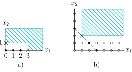
Figure 1: Standard monomials for Ideal(

D

) and Ideal(

C

). Both cases

were computed with a term order in which

x

> x

.

space bases of the quotient ring, calledstandard monomials, can be obtained from particular generating sets of Ideal(D), namely Gr¨obner bases and thus depend on a term ordering. The main steps of the computation are as follows.

1. Determine a Gr¨obner basis of Ideal(D) with respect to a term ordering, for example a Gr¨obner basis of Ideal(D1) is{x31−3/2x12+ 1/2x1, x1+x2−1}with respect to any term ordering for whichx2> x1;

2. compute the leading term of each element of the Gr¨obner basis, for the examplex31 and

x2;

3. determine all monomials which are not divisible by the leading terms, for the example 1,x1 andx21(see Figure 1a).

The CoCoA macros QuotientBasis performs the algorithm above. Models returned in Step 3. above have a hierarchical structure in that if they include the monomialxα _{then they}

also must includexβ _{for all β≤αcomponent-wise. A set of monomials with this property is}

Indeed for a mixture experiment D, the procedure above returns supports for slack models (Cornell, 2002, page 334). These can be homogenized to return the support for a homogeneous regression model Giglio et al. (2001). We could proceed differently and propose to adapt the above procedure to the homogeneous component of the design ideal, that is to work with the cone ideal instead of the design. The resulting homogeneous models can be different from those obtained by homogeneisation of a slack model as shown in Example 7.

There are two difficulties. First,R[x1, . . . , xk]/Ideal(CD) is infinite dimensional. Figure 1b) shows this for Ideal(CD1). Second, usually a polynomial does not define a polynomial function

onPk_{(R) equivalently on}

CD(see the comment before Definition 2). One classical CCA remedy to address the first problem considers only monomials of a certain degree say s ∈Z≥0. The basic algebraic definitions and results are in Appendices 8.2 and 8.4. Below we just apply them. For a mixture designD

1. determine a Gr¨obner basis of Ideal(CD) with respect to a term ordering, for Ideal(CD1)

it is{x1x22−x21x2};

2. compute the leading terms of each element of the Gr¨obner basis, for the examplex1x22 for term orderings for whichx2> x1;

3. consider all monomials of a sufficiently large total degree, for example inR[x1, x2] there are four monomials of degrees= 3, namelyx31, x21x2, x1x22, x32;

4. determine all monomials of degrees not divisible by the leading terms of the Gr¨obner basis, in the examplex31, x21x2, x32.

The monomials obtained in Step 4. above form a R-vector space basis of the quotient spaceR[x1, . . . , xk]s/Ideal(D)sand form a subset of the set of standard monomials for the cone

Lemma 3 LetDbe a mixture design ands∈Z≥0large enough. TheR-vector spaceR[x1, . . . , xk]≤s/Ideal(D)≤s has a basis[g1], . . . ,[gn]where representatives of the equivalence classes can be chosen to be

ho-mogeneous of degrees.

Theorem 4 LetDbe a mixture design. Then

dimR[x1, . . . , xk]s/Ideal(CD)s= dimR[x1, . . . , xk]≤s/Ideal(D)_≤s

If moreoverDhasndistinct points andsis sufficiently large then the dimensions equal n.

A monomial basis of degreescan be computed with the Singular macrokbase.

Example 6 The Gr¨obner basis of the homogeneous ideal ofD3 ={(0,0,1), (0,1,0),(1,0,0), (1/3,1/3,1/3)}and for any ordering for whichx1> x2> x3is{x1x3−x2x3, x1x2−x2x3, x22x3−

x2x23}. The leading terms arex1x3,x1x2,x22x3respectively. Fors= 3 the standard monomials are x31, x32, x33, x23x2: the largest possible number of terms we can identify with a four point design. Fors= 1 we obtained the support for a non saturated model: x1, x2, x3. Below we list the degreesstandard monomials for all values ofs.

s list of monomials of degrees degreesstandard monomials

0 1 1

1 x1, x2, x3 x1, x2, x3 2 x2

1, x1x2, x22, x1x3, x2x3, x23 x21, x22, x2x3, x23

3 x31, x21x2, x1x22, x32, x21x3, x31, x23, x2x23, x33

x1x2x3, x22x3, x1x23, x2x23, x33

s >3 xs

1, xs1−1x2, xs1−2x22, . . . , xs3 xs1, xs2, x2xs3−1, xs3

Example 7 The slack model obtained for D3 with respect to any ordering with x1 > x2 >

x3 has support 1, x3, x23, x2. By homogenising it following Giglio et al. (2001) we obtain

x3

1, x3x21, x32x1, x2x21, which is the support of a saturated homogeneous model of total degree 3 but different from the degree 3 model in Example 6. For slack models we consider “or-thogonal” projection over the axisxk = 0, while our procedure considers projection over the

Note the following things. i)Fors≥nthe procedure returns a degreessaturated support model. Example 6 shows that smaller values ofsare possible, but the returned model support may not be saturated. ii)Equivalently fors large enough, the design/model matrix forDand the degreesstandard monomials is invertible, and for anysit is full rank. iii)These standard monomials are not usually retrieved with the homogenization of a slack model, Example 7. iv)

Different identifiable models can be obtained by varying the term ordering, as in the affine case.

v)The degree sstandard monomial set can be used as a starting set to obtain other types of identifiable sets as shown in Section 3.1.

3.1

Changing model

Often we want to substitute standard monomials in the set obtained with the methodology of Section 3, or in any other monomial basis of the quotient space, with monomials from a set

δ that for some reason we would prefer to consider for the construction of the final regression model. The new set should still be a basis of the quotient space by Ideal(D). We present an algorithm to perform such substitution.

For a mixture design Dlet SMτ,s(CD) be the set of standard monomials of degreeswith respect to a term orderingτ. We simplify the notation SMτ,s(CD) to SMs. It seems reasonable

to start with a monomial set of the same size as the design, thus we takes sufficiently large. Setl=Pk

i=1xiand letGbe a Gr¨obner basis of Ideal(CD) with respect toτ.

Example 8 Our running example has D = {(1/4,1/4,1/2),(1/8,1/8,3/4), (1/3,1/3,1/3), (1/5,1/5,3/5),(0,0,1)},s= 4,τis the default term ordering in CoCoA andδ={x1, x2, x3, x1x2,

x1x3, x2x3, x1x2x3}is a Scheff´e type model (Scheff´e, 1963, page 237), Scheff´e (1958), (Cornell, 2002, page 334). Thus SMs={x42, x32x3, x22x23, x2x33, x43}.

Step 0. η:= SMsis the current monomial basis ofR[x1, . . . , xk]/Ideal(D),W :=∅set of

rewrit-ing rules,δ′_:=δ.

Compute the normal form ofwls−deg(w) _{with respect toG}

NF(wls−deg(w)_{) =} P

xα_∈SMsθαxα forθα∈R

= P

xα_∈ηθ

′

αxα

These equalities are valid over D. The second one follows by substituting the rules in

W where necessary (this can be cumbersome in practice).

Step 2. Chose a termxβ _inP

xα_∈ηθ

′

αxα for whichθ′β6= 0 and x β

6∈δ, equivalentlyxβ

∈SMs.

If there is not suchβthen repeatStep 1.

Step 3. Updateη:=η\{xβ

}∪{w}. In eachg∈W substitutexβ_with 1

θ′

β(w−

P

xα_∈η\{xβ_}θ′αxα)

and getg′_{. UpdateW ={x}β_≡ 1

θ′

β

(w−P

xα_∈η\{xβ_}θα′xα), g′:g∈W}.

Step 4. Repeat fromStep 1. untilδ′=∅.

This is a variation of the algorithm in Babson et al. (2003) where the setδis the union of all the stairs and their border sets. Stair is another name for an order ideal. The border of a monomial set is computed by multiplying any monomial in the set byxi, in turn fori= 1, . . . , k

and excluding monomials already in the set. The starting monomial set used in Babson et al. (2003), what we call η, is a stair as well. The correctness of the our algorithm is proved as for that in Babson et al. (2003). Its termination is guaranteed by the updating ofδ′ in Step 1. and the finiteness of δ. While in Babson et al. (2003) the algorithm terminates when η

containsnmonomials which are linearly independent and form an order ideal according to the chosen term ordering. In particular the algorithm in Babson et al. (2003) returns a support for a saturated hierarchical model. Different final monomial sets, and of possibly different sizes, might be obtained by choosing different monomials in Step 1. In the introduction we already mentioned the similarity with the algorithms in Faug`ere et al. (1993) and (Cox et al., 2004, Ch.8§5).

δ′=δ′\ {x1}. Steps 2. and 3. We selectxβ =x42 and updateη={x1, x32x3, x22x23, x2x33, x43} and W ={x4

2 ≡1/8x1−12/8x32x3−3/4x22x23−1/8x2x33}. Steps 1. and 2. Nextw=x2, updateδ′=δ′\ {x2}and NF(x2l3) = 8x42+ 12x32x3+ 6x22x23+x2x33=x1. There is no element to select as, over D, x1 = x2 which is already included in η. Steps 1. to 3. We try the next monomial in δ, w=x3 which can replacex32x3. We update η={x1, x3, x22x23, x2x33, x43},

W = W∪ {x3

2x3 ≡1/8x3−12/8x22x23−3/4x2x33−x43}and δ′. Steps 1. to 3. We update

ηsubstituting x2

2x23 withx1x2 and add the rulex22x23 ≡x1x2−x2x33−1/4x43−1/2x1+ 1/4x3 to W. Steps 1. to 3. Now we substitute in η the monomial x2x33 with x1x3 and add the rule x2x33 ≡ −1/16x43 + 4/9x1x2 + 2/9x1x2−2/9x1+ 4/243x3 to W. The current η is

{x1, x3, x1x2, x1x3, x43}. Steps 1. and 2. The next candidate inδ is x2x3. However, there is no interchange possible as over D,x2x3 =x1x3 and x1x3 ∈η. At this stepδ′ ={x1x2x3}.

Steps 1. to 3. The final monomial to be removed from η is x43 which is substituted with

x1x2x3. We add the rulex43 ≡6x1x2x3+ 14/3x1x2−11/3x1x3−7/3x1+ 235/162x3. Step

4. As now δ′ = ∅, the algorithm ends with the new model/representatives of classes of the quotient spaceη={x1, x3, x1x2, x1x3, x1x2x3}and with the updated set of rulesW to express polynomials in terms of monomials inη.

The starting monomial set does not need to be a SMs set but could be any other set of

monomials which are linearly independent overD. McConkey et al. (2000) McConkey et al. (2000) describe the confounding relationship between the parameters of the Scheff´e quadratic model and the model with supportxiandxi(1−xi),i= 1, . . . , kused to describe the average

deviation from linearity caused by an individual component on mixing with the other compo-nents. The setδcould then be this support and forw=xi(1−xi) the normal form ofxiP_j6=ixj

is computed.

SMτ ={1, x2, x3, x32}and anyτ for whichx1> x2> x3

B=

1 x2 x3 x23

x1 1 −1 −1 0

x2 0 1 0 0

x3 0 0 1 0

x1(1−x1) 0 0 1 −1

x2(1−x2) 0 0 1 −1

x3(1−x3) 0 0 1 −1

3.2

Rational models

Sets of linearly independent functions over D can be defined starting from a R-vector space basis ofR[x1, . . . , xk]/Ideal(D) and considering ratios of homogeneous polynomials of the same

degree.

Example 11 To D1 and {x1, x2, x1x2} we associate the real valued rational functions f1 =

x1 x1+x2, f2=

x2 x1+x2, f3=

x1x2

(x1+x2)2 where for example

x1

(x1+x2) : CD1 −→ R

(0,1) 7−→ 0 (1,0) 7−→ 1 (1,1) 7−→ 1/2

The design matrix ofD1 andf1, f2, f3 is the same as that ofD1 and x1, x2, x1x2. As overD1

x1+x2= 1, there is no issue in considering a polynomial model as usually done. Ifx1+x2=a for somea∈R\ {0}then a mixture-amount model either in polynomial form (Cornell, 2002,

§7.9) or rational form can be considered. The natural rational model which includes terms like

x1

a can be written as a polynomial model by introducing two extra indeterminates sayt= 1/a

and the extra polynomial ta−1. Namely, for θ1, θ2, θ11 parameters, θ1x1+θ2x2+θ11x1x2 becomes the rational modelθ1₍x1x+1x2)+θ2

x1

(x1+x2)+θ11 x1x2

(x1+x2)2 which in turn translates into

Sometimes in the literaturexiis substituted withxi/(1−xi) fori∈A⊆ {1, . . . , k}. These

functions are defined overDand not overCDand are used as screening models Cornell (2002). As the corner points with component 1 at the coordinates inA should not in the design, the normal forms (see Definition 6) of the polynomials 1−xi,i∈ A, are not zero. The authors

have not been able to prove of disprove the assertion that the linear independence of a set{xα_}

implies the linear independence of the “normalised”{xα_/Qk

i=1(1−xi)

αi_{}withα= (α}

1, . . . , αk).

An example is analysed in Section 5.2.

Some mixture model forms include inverse terms to model extreme changes in the response behaviour (see (Cornell, 2002, Ch.6)) for example

k

X

i=1

θixi+ k

X

i=1

θ−ix−i1 (1)

when no design point has a zero coordinate. Rather than checking that the design/model matrix is full rank we could employ a standard trick in algebra which allows us to transform the above in a polynomial model in two ways at least. Set yi = x−i1, to Ideal(D) add the

polynomials yixi−1, i = 1. . . , k and work in R[y1, . . . , yk, x1, . . . , xk] with a term ordering

which eliminates theyiindeterminates (Cox et al., 1997, page 72). Alternatively, rewrite Model

(1) asyPk

i=1θixi+Pki=1θ−iQjk6=i,j=1xj and add the polynomialyQki=1xi−1.

3.3

Logistic transformations

Mixture designs inRk+1with no point on the boundary are obtained from a full factorial designs in Rk _{by applying the additive logistic transformation or any other transformation that maps} Rk into the interior of the simplex in one higher dimension. Let F ⊂ Rk be a full factorial design withli1, . . . , lini∈Rlevels for factori. Then

Ideal(F) =h

n_i

Y

j=1

(zi−lij), i= 1, . . . , ki ⊂R[z1, . . . , zk] (2)

with the unique standard monomial set

(

zα:α∈

k

Y

i=1

{0,1, . . . , ni−1}

)

The additive logistic transformationxi=

ezi

1 +Pk j=1e

zj, fori= 1, . . . , kandxk+1=

1 1 +Pk

j=1e

zj

with inverse transformation

zi = ln

xi

xk+1

i= 1, . . . , k (4)

mapsz= (z1, . . . , zk) ∈ F into a mixture point. CallG the collection of such mixture points.

Note that substitution of the inverse relationship in (3) returns the support for a generalisation of the model (12.6) in Aitchison (1986).

Substitution of (4) in (2) and inclusion of the sum to one condition in thexispace gives

Ideal(G) =hPk+1

i=1xi−1,

Qni

j=1(xi−xk+1elij),i= 1, . . . , ki ⊂R[x1, . . . , xk+1].

Direct application of the Buchberger algorithm (Cox et al., 1997, Ch.2§7) shows that the polynomials above form a Gr¨obner basis for any term ordering for whichxk+1 > xi for all

i= 1, . . . , k. The corresponding standard monomial set is directly linked with the one of the full factorial in (3) and it gives the support for a slack model identified byG

{xα1

1 · · ·x

αk

k :αi∈ {0,1, . . . , ni−1}, i= 1, . . . , k} (5)

As another example of the simplicity and elegance of the algebraic statistics note that the recursive structure of the multiplicative logistic transformation xi =

ezi

Qi

j=1(1 +ezj) for

i= 1, . . . , k xk+1=_Qk 1

j=1(1 +ezj)

with inversezi= ln

xi

1−x1−. . .−xi

,i= 1, . . . , k sending

F intoHis reflected in the recursive structure of the polynomials in

Ideal(H) =h

k+1

X

i=1

xi−1, n_i

Y

j=1

“

xi(1 +elij)−(1−x1−. . .−xi−1)elij

”

: i= 1, . . . , ki

There exists at least a term ordering for which the leading terms of the polynomials above are

xni

i and for the sum to one condition it isxk+1. The corresponding standard basis is again (5) while the substitution of the inverse relationship in (3) returns the support for a generalisation of the model (12.7) in Aitchison (1986).

4

Some symmetric mixture designs

intercept are identifiable by such an experiment.

Lemma 5 Let D ⊂ Rk _{be the mixture design formed by the k corner points of the simplex} and τ be a term order. If xk > xi for all i∈ {1, . . . , k}, then the (generalised) confounding relationship for a general interactionxα=xα₁1. . . xαkk,α∈Z

k

≥0, is

NF(xα_{) =}

8 > > > > > > > > < > > > > > > > > :

1−Pk−1

i=1 xi ifxα=xαkk

xi ifxα=xi, i= 1, . . . , k−1

0 ifαhas at least two non zero components

1 ifα= (0, . . . ,0).

(6)

Theorem 6 LetDbe a mixture that contains the corner points. Letτ be a graded term ordering for whichxk> xifor alli. Then

1. 1, x1, . . . , xk−1 are linearly independent monomials overD,

2. the coefficient of the term1inNF(xαk k )is1,

3. the coefficient of the term1inNF(xα_{), with x}α

6

=xαk k is0.

4.1

Simplex lattice designs

In Scheff´e (1958) Scheff´e discusses uniformly spaced distributions of points on the simplex to explore the whole factor space and calls them simplex lattice designs. A {k, m} simplex lattice design is the intersection of the simplex inRk and the full factorial design ink factors and with them+ 1 uniformly spaced levels {0,1/m, . . . ,1}. It has `m+k−1

m

´

points. Directly from that description we deduce that for the {k, m} simplex lattice design, D, Ideal(D) =

hQm

j=0(x1−j/m), . . . ,

Qm

j=0(xk−j/m),

Pk

i=1xi−1iwhere the firstkpolynomials are a simple generating set of the full factorial design and the last one is the simplex condition.

D

Ideal(

C

)

Number of terms

{

k,

1

}

Ideal(

C

) =

h

x

x

:

i

6

=

j

i

{

k,

2

}

Ideal(

C

) =

h

x

x

−

x

x

, x

x

x

:

i

6

=

j

6

=

l

i

+

{

2

, m

}

Ideal(

C

) =

h

x

x

f

(

x

, x

)

i

Table 1: Ideal(

C

) for some simplex lattice designs

Theorem 7 The algebraic fan of a{k, m} simplex lattice design has sizek. Each one of its elements is the set of all monomials up to degreemink−1 factors.

Corollary 8 There are no other saturated hierarchical polynomial models identified by the

{k, m}simplex lattice design apart from those of Theorem 7.

By Theorem 1 Ideal(CD) is the radical of the ideal generated by the homogeneous poly-nomialsQm

j=0(xi−lj/m) fori= 1, . . . , k,l=Pk_i=1xi. Table 4.1 reports a Gr¨obner basis for

Ideal(CD) for various combinations ofkand m. It uses the following functions g(x1, x2, w) =

Qw

j=1(x1−mjx−2j)(x1−x2 m−j

j ) for w∈Z>0

f(x1, x2) =

8

> > > > <

> > > > :

1 ifm= 1

g(x1, x2, w) ifmodd,m6= 1 andw=⌊m/2⌋ (x1−x2)g(x1, x2, w) for meven andw=m/2−1

Example 12 For the{4,4}design, the binomialsx1x2−x3x4,x1x3−x2x4 and x1x4−x2x3 added to the generator set of the ideal of either the design or its cone, select the four corner points and the centroid point. They also establish that the terms in each binomial are confounded, take the same values over the selected fraction.

The polynomial (x1−x2)(x3−x4) selects the 15 points for whichx1=x2 orx3=x4, see Example 18. With respect to the default term ordering in CoCoA we obtain the support for a slack model 1, x4, x24, x34, x44, x3, x23, x2, x22, x32, x42, x3x4, x3x24, x2x4, x22x4.

For the same fraction and term ordering, the support for a homogeneous model of total degrees= 0, . . . ,4 is

s SMs

0 1

1 x1, x2, x3, x4 2 x2

1, x1x2, x22, x2x3, x23, x1x4, x2x4, x3x4, x24

3 x3

1, x21x2, x1x22, x32, x2x23, x33, x22x4, x2x3x4, x23x4, x1x42, x2x24, x3x24, x34

4 x4

1, x31x2, x21x22, x1x32, x42, x2x33, x43, x33x4, x22x24, x2x3x24, x23x24, x1x34,

x2x34, x3x34, x44

In Example 12 we had to take the saturation Hartshorne (1977) of the ideal generated by the homogeneous polynomialsQ4

j=0(xi−lj/4),i= 1,2,3,4 and (x1−x2)(x3−x4) with respect to x1, x2, x3, x4. The saturation is an algebraic operation which allows us to take the largest homogeneous ideal defined over a variety, namely the ideal of the variety. It can be performed in e.g. CoCoA with the commandSaturation. We do not study it here any further and refer to Hartshorne (1977), but we add another example and some comments in order to clarify the algebraic motivation.

Example 13 In P3 with coordinatesx, y, z, w consider the two skew lines L1 = V(x, y) and

L2 = V(z, w) and the curve C =L1∪L2 whose ideal is Ideal(C) = Ideal(L1)∩Ideal(L2) =

hxz, xw, yz, ywi. If we cutCwith the planeH = V(y+z) we obtain two pointsA1= (0 : 0 : 0 : 1) and A2 = (1 : 0 : 0 : 0) whose ideal is Ideal(A1, A2) =hy, z, xwi. Of course it is natural to compute the ideal J = Ideal(C) + Ideal(y+z) more than the coordinates of the intersection

Clearly J 6= Ideal(A1, A2) and it is easy to verify that Js = Ideal(A1, A2)s for s ≥ 2.

So, we can say that the sum of the two ideals I and J is asymptotically equal to the ideal of the intersection of the varieties V(I) and V(J). In fact, when we compute combinations of homogeneous polynomials we get always polynomials of degree larger than or equal to the degree of the operands.

The algebraic operation that allows us to compute the ideal of V(I)∩V(J) fromI+J is thesaturation with respect to the ideal generated by all the indeterminates, and it consists in looking for homogeneous polynomialsfwith the property thatf xmi

i ∈I+Jfor somemi∈Z>0 and for everyi= 1, . . . , k.

In the affine space this phenomenon does not show up because when computing combi-nations of non homogeneous polynomials we can obtain polynomials of degree strictly smaller than the degree of the operands.

4.2

Simplex centroid designs

Simplex centroid designs introduced in Scheff´e (1963) are mixture designs in which coordinates are zero or equal to each other. Thus in thekdimensional simple centroid design there arek

points of the form (1,0, . . . ,0),`k

2

´

of the form (1 2,

1

2,0, . . . ,0),

`k

3

´

of the form (1 3,

1 3,

1

3,0, . . . ,0), ..., and the point (1

k, . . . ,

1

k): a total of

Pk j=1

`k j

´

= 2k

−1 points. This design is the projection of the full factorial design with levels 0 and 1, on the simplex inRk with respect to the origin. Again easily we see that there are 2k

−1 points. We rename “2k_{design” the full factorial design}

with levels 0 and 1 ink factors.

The ideal of the cone of D is Ideal(CD) = hx2ixj−xix2j : i, j = 1, . . . , k;i 6= ji. The

geometry of the design is easily deduced by inspection of the factorised generatorsxixj(xi−xj):

coordinates of a point in Dare either 0 or equal to each other. The generator set given for Ideal(CD) is a Gr¨obner basis with respect to any term ordering. The proof is a straightforward application of the S-polynomial test (Cox et al., 1997, Ch.2§6Th.6).

Also the construction of Ideal(D) can be based on the derivation of the simplex centroid design from the 2k _{design but it is more complicated and involves techniques from elimination}

to list the mixture point coordinates. The steps of the constructions are as follows.

1. The ideal of the 2k_{design is}

hx2

i−xi:i= 1, . . . , ki.

2. The origin can be removed by adjoining the polynomial given by the sum of the ele-mentary symmetric polynomials and 1 with alternate signs (Cox et al., 1997, Ch.7§2). The elementary symmetric polynomials inR[x1, . . . , xk] are σ1 = (x1+. . .+xk), . . .,

σr= (P_i

1<i2<···<irxi1. . . xir),. . .,σk= (x1. . . xk).

3. The simplicial projection is performed in two steps Bocci et al. (2005). Extend the poly-nomial ring with the variablesy1, . . . , ykand adjoin to the ideal above the polynomials

yi(Pk_j=1xj)−xi.

4. Eliminate the indeterminatesxi, i= 1, . . . , k from the ideal obtained in 3. above (Cox

et al., 1997, Ch.3) to get Ideal (D) which is now expressed in theyiindeterminates.

Example 14 Fork= 3 the affine ideal of a 23 _{design ishx}2

1−x1, x22−x2, x23−x3i. The origin is removed with the ideal operation Ideal(23\ {(0,0,0)}) = Ideal(23) +hσ3−σ2+σ1−1i, where

σ3−σ2+σ1−1 =x1x2x3−x1x2−x1x3−x2x3+x1+x2+x3−1. Extend the polynomial ring withy1, y2, y3and create the following ideal: Ideal(23\{(0,0,0)})+hy1l−x1, y2l−x2, y3l−x3i ⊂

R[x1, x2, x3, y1, y2, y3], where l=x1+x2+x3. Eliminate the variables x1, x2, x3, for instance with the CoCoA macroElim. This last step gives a set of generators for Ideal(D){y1+y2+y3− 1, y3(y3−1)(2y3−1)(3y3−1), y2y3(y2−y3), y3(2y3−1)(2y2+y3−1), y2(2y2−1)(y2+2y3−1)}.

In Scheff´e (1963) Scheff´e considers two types of fractions of a simplex centroid. A fraction

Dof the type in (Scheff´e, 1963,§Appendix B) is built from a fraction of the 2k _design,

F not including the origin. In this case Ideal(D) is computed starting the above algorithm with F

and by homogenization as in Theorem 2 Ideal(CD) can be obtained. The ideal of a fraction of the other type (Scheff´e, 1963,§5) is built starting the algorithm from an echelon fraction of the 2k_{design excluding the origin. For echelon designs see (Pistone et al., 2001,}

Example 15 For 1< m≤kletFmbe the fraction of a simplex centroid design that includes

all points with at mostmnon zero components, whereFk is the full simplex centroid. Clearly,

Fm satisfies the description in (Scheff´e, 1963, §5). The number of points inFm is Pmj=1

`k j

´

. The cone ideal forFmishx2ixj−xix2j, xi1· · ·xim+1:i6=jandi1=6 · · · 6=im+1iifm >1 which

for m= 1 simplifies to hxixj :i6=ji. Differently from Example 12 the given generators are

those of a saturated ideal.

Example 16 We compute the algebraic fan of D = Fm of Example 15 as an example of

the application of the techniques in Subsection 4.2. First note that the given generator set is a universal Gr¨obner basis. Form= 1 and any term ordering, the leading term ofxixj∈Ideal(CD) is the monomial itself. Thus the homogeneous model has support {xs

1, xs2, . . . , xsk} for any

s ∈ Z≥1. If m > 1 the leading term of xi1xi2· · ·xim+1 is the monomial itself. For a given

initial term ordering onx1, . . . , xk, e.g. x1 < x2< x3, the leading term ofxi2xj−xix2j isx2ixj

ifxi> xjandxix2j otherwise. For a given initial term ordering there are

Pm j=1 `k j ´ monomials of total degree snot divisible by x2ixj, with xi > xj and xi1xi2· · ·xim+1, namely form = 3

{xs

i, xsi−1xj, x s−2

i xjxl:i, j, l= 1, . . . , k, i < j < l}.

4.3

Snee-Marquardt designs

In Snee and Marquardt (1976) simplex screening designs which are axial designs are presented and now they are known as Snee-Marquardt designs. The Snee-Marquardt design inkfactors,

M, is formed by the points

kvertices (1,0, . . . ,0), . . . ,(0, . . . ,0,1) 1 centroid (1

k, . . . ,

1

k)

kinterior points (k+1 2k ,

1 2k, . . . ,

1 2k), . . . ,(

1 2k, . . . ,

1 2k,

k+1 2k )

kend effects (0, 1

k−1, . . . , 1

k−1), . . . ,( 1

k−1, . . . , 1

k−1,0)

To construct Ideal(M) observe that each point inMlies on the lineAithrough Theith

vertex and its opposite end effect point, fori= 1, . . . , k. The ideal Ideal(M ∩ Ai) is generated

byg = Pk

obtained by changing thefi polynomials. First we prove that ifh, l are different fromi, then

xixl(xi−(k+ 1)xl)(xi−xl) andxixh(xi−(k+ 1)xh)(xi−xh) cut Ai on the same subset.

This remark justifies the fact that, in our notation,fi does not depend onl. In fact, it holds

xixl(xi−(k+ 1)xl)(xi−xl)−xixh(xi−(k+ 1)xh)(xi−xh) = (xl−xh)xi[x2i−(k+ 2)xi(xl+

xh) + (k+ 1)(x2l +xlxh+x2h)] ∈Ideal(Ai). The ideal definingMis the intersection of the

Ideal(M ∩ Ai)’s. As usual we compute Ideal(CM). If k = 3, a straightforward computation shows that Ideal(CM) =h(x1−x2)(x1−x3)(x2−x3), x1x2(x1−x2)(x1+x2−5x3), x1x3(x1−

x3)(x1+x3−5x2), x2x3(x2−x3)(x2+x3−5x1)i. Next, we want to compute a finite generating set of Ideal(CM) fork≥4.

Proposition 1 Fork≥4, Ideal(CM) is generated byqijkl= (xi−xj)(xh−xl) wherei, j, h, l are different from each other in{1, . . . , k}and byfrs=xrxs(xr−xs)(xr+xs−(k+ 1)xt)), wherer, s, tare different from each other in{1, . . . , k}.

A corollary of Proposition 1 is that

HFIdeal(CM)(s) = 8

> > > > > > > > > > > <

> > > > > > > > > > > :

1 ifs= 0

k ifs= 1 2k ifs= 2 3k ifs= 3 3k+ 1 ifs≥4

5

Notes on the analysis of two data sets

5.1

A non regular mixture design

Initial model

Final terms

R

_R

A

σ

ˆ

×

10

M

h

, bh, df, eh

0

.

977 0

.

958 6

.

1

M

f, h, bh, f h

0

.

983 0

.

978 4

.

4

M

,

2

(1−g)2

,

bh

(1−b)(1−h)

,

0

.

974 0

.

964 5

.

7

ch

(1−c)(1−h)

,

gh

(1−g)(1−h)

Table 2: Results of model selection

In particular we may want to check if we can replace the quadratic terms of f2_{, g}2_{, h}2 _{by the} linear termsf, g, h. Indeed that is the case and we have a (more) Scheff´e (like) model, named M2. We could as well have replaced some interactions terms with linear terms, for example building models degree by degree using a suitableδset in the algorithm in Subsection 3.1. But we do not pursue this here. Finally, following Cornell (2002) we can construct a support for a third model wherexixj in M1 are replaced by the rational termsxixj/((1−xi)(1−xj)). We

refer to this model as M3. Such a substitution with rational terms is not always possible. But in this specific example it can be shown that the linear independence of the terms in M3 over the design follows from the linear independence of the terms inM1, because of the particular structure of the design.

For practical purposes, often a reduced model which fits reasonably well to the data, is preferred to the saturated one. Table 5.1 shows the values of the determination coefficientR2, the adjusted oneR2

Aand the residual error ˆσfor the submodels obtained with backward stepwise

regression. We use theleapsfunction in the statistical softwareR; see http://cran.r-project.org.

5.2

A fraction of the simplex centroid design

factors such that any pair of non zero factors appears in the design just once. The fact that there are many such fractions, obtained by relabeling of the factors is clearest from the structure of the polynomial representation below. The fraction obtained is of the echelon type described in (Scheff´e, 1963,§5), and it is labeled{k|p}in McConkey et al. (2000). In McConkey et al. (2000) it is noted that there are some values ofk for which a {k|p}fraction cannot be constructed. We focus our attention on the{9|3}analysed in McConkey et al. (2000). To construct the cone ideal consider the polynomials

xi(xj−xk), xj(xi−xk), xk(xj−xi) : (i, j, k)∈A and xixj(xi−xj) :i6=j, i, j∈ {1, . . . ,9}

where the second set of polynomials gives the simplex centroid design in 9 factors and the set A = {(1,2,3),(1,4,8),(2,5,9),(3,6,7),(4,5,6),(2,4,7),(3,5,8), (1,6,9),(7,8,9), (1,5,7), (2,6,8),(3,4,9)}corresponds to the non-zero triplets in our design. The centroid point (1 :. . .: 1) still satisfies that set of equations. The algebraic operation to remove it is thecolonof ideals (Cox et al., 1997, Ch.4§4) and can be achieved by taking the saturation of the ideal generated by the above polynomials andx1x2x3x4x5x6x7x8x9 or any other degree three monomial with exponents not inA, for examplex4x8x9, where the saturation is with respect to the usual ideal Ideal(x1, . . . , x9). The Hilbert function (Appendix 8.4) of the cone ideal is

HFIdeal(CD)(s) = 8

> > > > <

> > > > :

1 ifs= 0 9 ifs= 1 21 ifs≥2

and thus we can construct a saturated homogeneous model of degree two. For the default term ordering in CoCoA withx1> . . . > x9 the support for such a model is

{x2

1, x22, x2x3, x23, x24, x4x7, x4x8, x4x9, x25, x5x6, x5x7, x5x8, x5x9, x26,

x6x7, x6x8, x6x9, x27, x28, x8x9, x29}

(7)

A feature of a {k|p} fraction is that double interactions are completely confounded over the design in sets of sizep, e.g. for the{9|3}fraction the polynomialsx1x2−x1x3, x1x2−x2x3 and

x1x3−x2x3belong to Ideal(CD), that is the column of a design/model involving the polynomials

The termsxican replace the termsx2i in Equation (7), e.g. by application of the algorithm

in Section 3.1. The design/model matrix for the obtained model and the fraction {9|3} is a diagonal matrix of the form

2

6 4

I9 0

P 1 9I12

3

7 5

whereIk is the identity matrix of sizek andP is the 12×9 matrix listing the coordinates of

the mixture points.

6

Further comments

If the points ofDdo not lie on a hyperplane, none of them is the origin and each line through the origin and a design point does not contain any other design point, then the cone ideal is still well defined. The identifiability theory of homogeneous model supports works exactly as for mixture designs. In particular Ideal(CD) is the largest homogeneous ideal in Ideal(D). Although mathematically sensible, this operation does not seem to be reasonable if the design points do not lie on a hyperplane.

For an experiment where the relative proportions of the components are significant rather than the total amount, few relevant facts are implied by considering the cone ideal. The design points are recovered as the variety obtained from intersecting the cone ideal with the simplex ideal as shown in Theorem 1. The generalised confounding relationships collected in Ideal(CD) are the same whatever the total amount of the mixture is. Likewise the homogeneous model supports are independent of the total mixture amount.

Both the confounding relationships and the model support are easily computed even for fairly irregular designs, i.e. designs that do not manifest any geometric symmetry. An exact evaluation of the speed of the algorithms in function of the sample size and number of factors has not been done. An estimation can be obtained from Abbott et al. (2000). Macros in the computational algebra package CoCoA to compute homogeneous model supports, the ideals and the cone ideals of the designs in Section 4 are available from the first author.

to identifiability. Thus numerical approximations are postponed to the estimation phase of an analysis. For example rather than checking numerically if the rank of the design/model matrix for a candidate model is maximal, one computes a basis of the quotient space. This might be advantageous or disadvantageous according to the practical situations. We find that the information embedded in the ideal of a design or of its cone are useful in visualising the constraints imposed on the power terms by the design.

7

Acknowledgments

The authors thank Prof. H. P. Wynn and A. di Bucchianico for providing initial bibliographical references on mixture designs. The first author acknowledges financial support from CONA-CYT.

8

Appendix

Reference texts for this appendix include Adams and Loustaunau (1994); Cox et al. (1997); Kreuzer and Robbiano (2000).

8.1

Basic concepts

WithR[x1, . . . , xk] we indicate the set of polynomials inx1, . . . , xk and with real coefficients.

The theory holds for whatever fieldKinstead ofR. For usTkindicates the set of power products or monomials inR[x1, . . . , xk]: xα=xα₁1. . . x_kαkforαi∈Z≥0and a polynomialf∈R[x1, . . . , xk]

is a finite sumf=P

α∈Aaαxα withxα∈Tk,aα∈Rand for a finite subsetA⊂Zk≥0.

Definition 3 A setI ⊂R[x1, . . . , xk]is a polynomial ideal if i)f+g∈I for allf, g∈I and ii)hf∈I for allh∈R[x1, . . . , xk]andf∈I.

Theorem 9 Every idealI ⊆R[x1, . . . , xk] is finitely generated, i.e. there exist g1, . . . , gt ∈I such that for everyf∈I there existh1, . . . , ht∈R[x1, . . . , xk]that satisfyf=h1g1+· · ·+htgt.

The polynomialsg1, . . . , gt in the previous theorem form a set of generators ofI and we write

I=hg1, . . . , gti. There are special sets of generators called Gr¨obner bases. To introduce them

we need the notion of term ordering. A term orderingτ is a total order relation on Tk _that

satisfies i) xα _{> 1 for all non zero α ∈ Z}k

≥0 and ii) if xα > xβ then xαxγ > xβxγ for all

α, β, γ∈Zk≥0.

Definition 4 Given a term ordering τ, the leading term of a polynomial f ∈R[x1, . . . , xk]is its largest term with respect to τ, and we write it asLTτ(f).

Given a term orderingτ and an idealI, we consider the set of leading terms of all polynomials inI: LTτ(I) =hLTτ(f) :f∈Ii. Ifg1, . . . , gtis a generator set of an idealI, in general LTτ(g1),

. . . ,, LTτ(gt) is not a set of generators of LTτ(I). This remark justifies the following definition.

Definition 5 LetI be an ideal, τ a term ordering and G={g1, . . . , gt} ⊆I. Gis a Gr¨obner basis (sometimes called a standard basis) ofI ifLTτ(I)is generated byhLTτ(g) :g∈Gi.

Theorem 10 For every idealI and term ordering τ there exist Gr¨obner bases ofI.

Definition 6 Letr=P

α∈Aaαx

α _{be a polynomial,τ a term ordering and I be an ideal. r is}

in normal form w.r.t. I andτ ifxα_6∈LT

τ(I)for allα inA.

The following result holds.

Proposition 2 Letτbe a term ordering,Ian ideal and letG={g1, . . . , gt}be a Gr¨obner basis ofI w.r.t. τ. For every polynomialf∈R[x1, . . . , xk]there exists a uniquer∈R[x1, . . . , xk]in normal form and h1, . . . , ht ∈R[x1, . . . , xk]such thatf =h1g1+· · ·+htgt+r. Furthermore,

r= 0 if and only iff∈I.

Given an idealI, we can consider the quotient ringR[x1, . . . , xk]/Iwhose elements are the

by polynomials obtained as combination of terms not in LTτ(I). The set SMτ(I) =Tk\LTτ(I)

is called the set of the standard monomials ofI w.r.t. τ. As R-vector spaces,R[x1, . . . , xk]/I

is isomorphic to R[x1, . . . , xk]/LTτ(I) and so it is isomorphic to the vector space spanned by

SMτ(I) overR. The Singular macrokbasisreturns SMτ(I) for an ideal of points.

8.2

Affine Hilbert function for ideals

Fors∈Z≥0letR[x1, . . . , xk]≤s= Span(xα∈Tk:Pki=1αi≤s). For an idealI⊂R[x1, . . . , xk],

let I≤s =I∩R[x1, . . . , xk]≤s. As R[x1, . . . , xk]≤s is aR-vector space of dimension`k+_ss´ and

I≤sis a subvector space ofR[x1, . . . , xk]≤s, we can define theaffine Hilbert functionofI as

a_HF

I(s) = dimR[x1, . . . , xk]≤s/I≤s= dimR[x1, . . . , xk]≤s−dimI≤s.

There existss0called theindex of regularity ofIsuch that for alls≥s0aHFI(s) is a polynomial

with integer coefficients. It is called theaffine Hilbert polynomialofIand denoted asa_HP

I(s).

That is

a_HP

I(s) = k

X

i=0

bi

s k−i

!

withbi∈Z≥0andbi>0. The following theorem gives the affine Hilbert function for the design

idealI(D).

Theorem 11 LetI(D) be the ideal generated by a designD withn distinct points. Then for

s≥n,a_HF

I(D)(s) =aHPI(D)(s) =n.

Proof. This is in (Cox et al., 1997, Ex.10,Ch.9§4).

The Hilbert function counts the monomials that are not in I(D); this set of monomials is precisely the set of standard monomials as described in Subsection 8.1. AsaHPI(D)(s) is a constant, we retrieve the standard result dimR[x1, . . . , xk]/I=n.

A term ordering τ is graded if xα _{is larger thanx}β _wheneverPk

i=1αi>Pk_i=1βi. Letτ

be a graded term ordering, then for alls∈Z≥0

a_HF

8.3

Homogenising a mixture ideal

A key point in this paper is the study of mixture designs through cone ideals, namely Ideal(CD)⊂

R[x1, . . . , xk] for a mixture design D. As mentioned in the main text, there are macros e.g.

IdealOfProjectivePointswhich construct a generator set for Ideal(CD) from the coordinates ofD. Next we outline the basic construction of Ideal(CD) which can be performed in any software for ideal computation. LetD={P1, . . . , Pn}be the design and assume thatPi= (ai1, . . . , aik)

with Pk

j=1aij = 1. Then, Pi belongs to the hyperplane H defined by the single equation

x1+. . .+xk= 1 fori= 1, . . . , n. MoreoverPiis the intersection ofHwith the lineLicontaining

Pi and the origin 0 = (0, . . . ,0). In particular, we have Ideal({Pi}) =hIdeal({Li}), x1+. . .+

xk−1i. But Ideal(D) = T_in₌₁Ideal({Pi}) = hTn_i=1Ideal({Li}), x1+. . .+xk−1i. We set

Ideal(CD) = Tni=1Ideal({Li}), and so Ideal(D) = hIdeal(CD), x1+. . .+xk−1i. Now, we

describe some properties of Ideal(CD).

Theorem 12 Ideal(CD)is generated by homogeneous polynomials.

Proof. The ideal defining the linesLiis generated by the 2×2 minors of the matrix

0

B @

x1 . . . xk

ai1 . . . aik

1

C A

and so it is generated by homogeneous linear polynomials. The intersection of ideals generated by homogeneous polynomials is again generated by homogeneous polynomials. So the claim follows.

Ideal(CD) can be characterized as follows.

Theorem 13 Ideal(CD)is the largest homogeneous ideal inIdeal(D).

Proof. Let f ∈ Ideal(D), f homogeneous. Then f(tai1, . . . , tsik) =tdegff(ai1, . . . , fik) = 0

for every i = 1, . . . , n and for all t ∈ R. Hence, f ∈ Ideal({Li}) for all i = 1, . . . , n and so

8.4

Hilbert function

An idealIh

⊂R[x1, . . . , xk] is homogeneous if it is generated by a set of homogeneous

polynomi-als. Fors∈Z≥0letR[x1, . . . , xk]s= Span(xα∈Tk:Pki=1αi=s)∪ {0}and for a homogeneous

ideal Ih

⊂ R[x1, . . . , xk], let Ish = Ih∩R[x1, . . . , xk]s. R[x1, . . . , xk]s is a R-vector space of

dimension`k+s−1

s

´

andIshis a subvector space. The Hilbert function of the homogeneous ideal

I is HFI(s) = dimR[x1, . . . , xk]s/Ish.

Theorem 14 LetIh

⊂R[x1, . . . , xk]be a homogeneous ideal.

1. For s sufficiently large HFIh(s) is a polynomial with rational coefficients and integer values.

2. Fors≥1

HFIh(s) =aHFIh(s)−aHFIh(s−1) (8)

3. IfIh _{is a monomial ideal and thus trivially homogeneous, thenHF}

Ih(s) is the number of monomials not inIh_{and in}

R[x1, . . . , xk]s.

4. Ifτ is a term ordering andIh_{a homogeneous ideal, then HF}

Ih(s) = HF_hLT(Ih_)i(s).

5. (The dimension theorem) Let V = V(I) = ˘

a∈Pk−1(C) :f(a) = 0for allf∈I¯

be

non empty. Thendim(V) = deg HPI(s)wheredim(V), forV a projective variety, is de-fined as the degree of the Hilbert polynomial ofI. Furthermore,dim(V) = deg HPhLT(I)i(s)

equals the maximum dimension of a projective coordinate subspace in V(hLT(I)i). If

I= Ideal(V) the last statements hold over R.

6. The previous statement holds forIan ideal, not necessarily homogeneous,V =V(I)and

HPI(s)is substituted byaHPI(s)

For the proof we refer to any classical text such as Cox et al. (1997). Here we just need to observe that as we deal with a regular structure asV =CDthenI= Ideal(V).

×

x

x

0 1 2 3

1

2

3

4

5

s

= 5

LT

a)

×

x

x

s

= 5

s

= 4

b)

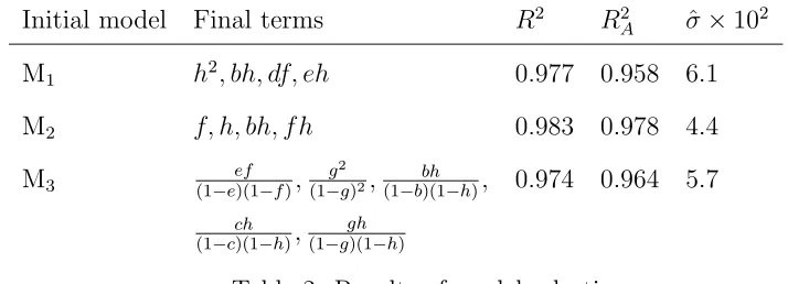
Figure 2: Standard monomials counted by a) the Hilbert function with

s

= 5 and b) the affine Hilbert function for

s

= 4

,

5. Both cases refer to

I(

C

) of Example 17.

ideal can be retrieved by Equation (8) together with the initial condition aHFIh(0) = 1. If

the ideal is not homogeneous then Hilbert returns the Hilbert function of the corresponding leading term ideal w.r.t. whatever term ordering is running in the open computer session.

Example 17 For D = {(1/2,1/2),(1/4,3/4),(0,1)} and a term order in which x1 > x2, Ideal(CD) =hx31−4/3x21x2+ 1/3x1x22i. Compare the following table with Figure 2

s HFIdeal(CD)(s)

a

HFIdeal(CD)(s)

0 1 1

1 2 3

2 3 6

3 3 9

4 3 12

..

. 3 3 +a_HF

Ideal(CD)(s−1)

Theorem 15 Let D be a mixture design with n distinct points and let CD be its cone; let Ideal(D) andIdeal(CD) be their corresponding ideals. Then fors large enough, HFI(CD)(s) =

a_HF

I(D)(s).

Example 18 The Hilbert function of the cone ideal of the{4,4}design in Example 12 is

HFIdeal(CD)(s) = 8 > > > > > > > > > > > < > > > > > > > > > > > :

1 ifs= 0 4 ifs= 1 10 ifs= 2 20 ifs= 3 35 ifs≥4

For the fraction cut by (x1−x2)(x3−x4) it is

HFIdeal(CF)(s) = 8 > > > > > > > > > > > < > > > > > > > > > > > :

1 ifs= 0 4 ifs= 1 9 ifs= 2 13 ifs= 3 15 ifs≥4

We use the CoCoA macroHilbert.

8.5

Proofs

Proof. of Theorem 1. 1. Let f ∈ I = {f ∈ R[x1, . . . , xk] : fis homogeneous andf(d) =

0 for alld ∈ D}. As f is homogeneous thenf(αd) = 0 for all α∈ Rand thus f(d) = 0 for

d∈ CD. HenceI⊆Ideal(CD).

Now we show that Ideal(CD) is homogeneous. Iff ∈ R[x1, . . . , xk] andf(d) = 0 on the

cone then asD ⊂ CDf(d) = 0 onD. Any polynomialfcan be written asf=fs+fs−1+· · ·+f0 withfi homogeneous polynomials of degreei. Forα∈Randd∈Rk

f(αd) =fs(αd) +fs−1(αd) +· · ·+f0(αd) =αsfs(d) +αs−1fs−1(d) +· · ·+α0f0(d) (9)

If we takef vanishing onCDthen we have f(αd) = 0 for allα∈Rand d∈ D. Equation (9) is a polynomial of degrees in α. As it is zero for infinitely manyα’s then its coefficients are zero that is fs(d) = . . . = f0(d) = 0. In particular for all d ∈ D. As by constructionfi is

homogeneous,f (d) = 0 for alldin the cone. Hence Ideal(C ) +hPk

2. Clearly Ideal(CD) ( Ideal(D) ⊂ R[x1, . . . , xk] and hPki=1xi −1i ( Ideal(D) ⊂ R[x1, . . . , xk]. Hence, Ideal(CD) +hPk_i=1xi−1i ⊆Ideal(D).

Let g ∈ Ideal(D). Then there exists s ∈ Z≥0 such that g = Psi=0fi and the fi’s are

homogeneous polynomials of total degree i. AsPk

i=1xi−1 ∈Ideal(D) we set

Ps

i=0fi(x1+

· · ·+xk)s−i=h(g) overD. Then, forl=x1+· · ·+xk

g−h(g) = g−Ps

i=0fi(x1+· · ·+xk)s−i=g−Psi=0fils−i

= (1−l)`

fs−1+ (1 +l)fs−2+· · ·+ (1 +l+· · ·+ls−1)f0

´

= (1−l) ¯f

and we haveg−h(g) = ¯f(1−l). But bothgand (1−l) ¯fare in Ideal(D), thush(g)∈Ideal(D). By 1. h(g)∈Ideal(CD) and thusg∈Ideal(CD) +hl−1iand the the proof is concluded. Proof. of Theorem 2. Letf ∈Ideal(D) be a homogeneous polynomial of degrees. From the defining property of a Gr¨obner basis, there exist q, q1, . . . , qr ∈ R[x1, . . . , xk] such that

f =q(l−1) +q1g1+. . .+qrgr with degq≤s−1 andδi = deg(qigi)≤s. Homogenising we

obtainh(f) =h(q)h(l−1) +ls−δ1_h(q

1)h(g1) +. . .+ls−δrh(qr)h(gr) and of courseh(l−1) =

l−l = 0. Thus h(f) = Pr i=1l

s−δi_h(q

i)h(gi). But f is homogeneous and so f = h(f) and

f=Pr i=1l

s−δi_h(q

i)h(gi). The claim now follows from Theorem 1.

Proof. of Lemma 3. Let [f] be an element in R[x1, . . . , xk]≤s/Ideal(D)≤s. We want to

prove that there exists g ∈ [f] such that g is homogeneous of degree s. Letl =x1 +. . .+

xk and let f = ft+. . .+f0 where fj is homogeneous of degree j and t ≤ s. Let g =

ls−t`

ft+lft−1+. . .+ltf0

´

ls−t_{h(f). Then,}

g−f = ls−t`

ft+lft−1+. . .+ltf0

´

−`

ft+lft−1+. . .+ltf0

´

+`

ft+lft−1+. . .+ltf0´−(ft+. . .+f0) = (ls−t

−1)`

ft+lft−1+. . .+ltf0

´

+ (l−1)ft−1+ (l2−1)ft−2+. . .+ (lt−1)f0 = (l−1)ˆ

(ls−t−1+. . .+ 1)`

ft+lft−1+. . .+ltf0´ +ft−1+ (l+ 1)ft−2+. . .+ (lt−1+. . .+ 1)f0˜

Butl−1∈Ideal(D) and sog∈[f].

Proof. of Theorem 4. Let [f1], . . . ,[fp] be a basis of theR-vector spaceR[x1, . . . , xk]≤s/Ideal(D)_≤s

and letg1, . . . , gpbe the degreeshomogeneous polynomials constructed in Lemma 3. We want

assume there existλ1, . . . , λp∈Rsuch thatλ1[g1] +. . .+λp[gp] = 0. Thenλ1g1+. . .+λpgp∈

Ideal(CD) ⊆Ideal(D) and soλ1[g1] +. . .+λp[gp] = 0 in R[x1, . . . , xk]≤s/Ideal(D)_≤s. Hence,

λ1[f1] +. . .+λp[fp] = 0 and so λ1 = . . . = λp = 0 because [f1], . . . ,[fp] is a basis of R[x1, . . . , xk]≤s/Ideal(D)_≤s.

Let g ∈ R[x1, . . . , xk]s. Thus, there existλ1, . . . , λp ∈ Rsuch that [g] = λ1[f1] +. . .+

λp[fp] =λ1[g1]+. . .+λp[gp] and so [g1], . . . ,[gp] are generators ofR[x1, . . . , xk]s/Ideal(CD)s. As a

consequence, we get the claim. Ifsis sufficiently large then dimR[x1, . . . , xk]≤s/Ideal(D)_≤s=n

(see e.g. Pistone and Wynn (1996)) and thusp=n.

Proof. of Theorem 5. It is easy to show that Ideal(CD) is generated byhxixj : 1≤i, j ≤

k, i6=ji and so Ideal(D) =hx1+. . .+xk−1, xixj : 1≤i, j ≤k, i 6=ji. A Gr¨obner basis of

Ideal(D) contains also the polynomialsx2

i−xi, obtained from the S-polynomial test (Cox et al.,

1997, Ch.2§6Th.6) asxi(x1+. . .+xk−1)−Pi6=jxixj. The result now follows easily. Proof. of Theorem 6. For 1. observe that as the term ordering is graded then lower order terms are favoured over higher order terms and then included in the support for a slack model. It follows directly from the structure of the design/model matrix involved

x1 . . . xk−1 1 · · · (1,0, . . . ,0) 1 0. . . 0 1 · · ·

..

. 0

(0, . . . ,1,0) 0 0. . . 1 1 · · ·

(0, . . . ,0,1) 0 0. . . 0 1 · · ·

.. . For 2. let NF(xαk

k ) =

P

xαθαxαwhere for a slack support noxαinvolvesxkand evaluate it at

the corner pointck= (0, . . . ,0,1). Deduceθ0= 1. Similarly 3. is proved.

Lemma 16 Let D be a {k, m} simplex lattice design. Then a basis of the R-vector space R[x1, . . . , xk]≤s/Ideal(D)≤sis{1, x2, . . . , xk, x22, x2x3, . . . , x2k, . . . , xs

′

2, xs

′

2x3, . . . , xs

′

k}wheres′=

min{s, m}.

polynomials in Ideal(CD) by Theorem 1. Thus, letf∈Ideal(CD)m. We want to prove thatf= 0

and we use induction onk andm. The base of the induction is as follows. First, we analyse the case{2, m}, for whichD={P0, . . . , Pm}withPi= (i/m,(m−i)/m) fori= 0, . . . , m. But

no homogeneous polynomial of degree m can have m+ 1 distinct zeros, unless it is the null polynomial. Second, we consider the case{k,1}. But this design was studied in Lemma 5.

Now, we consider the general case{k, m}and we assume that no polynomial of degreem−1 belongs to a{k, m−1}design and that no polynomial of degreembelongs to a{k−1, m}design. Letf∈Ideal(CD)m. We need to show thatf= 0. If we setxk= 0 then we obtain a{k−1, m}

designD′ _{and f(x}

1, . . . , xk−1,0) ∈Ideal(CD′ )m. By inductive hypothesis,f(x1, . . . , xk−1,0) is the zero polynomial. Hence,f=xkf′for somef′suitable homogeneous polynomialf′of degree

m−1. The affine transformation,Xi=_mm₋₁xi,i= 1, . . . , k−1 andXk=−_m1₋₁+_mm₋₁xk, takes

D \D′_{into a{k, m−1}simplex lattice design, sayD}′′_{, andf}′_into“ m m−1

”m−1

f′(X1, . . . , Xk−1)

∈ Ideal(D′′_{). By inductive hypothesis, we have f}′ _{= 0 and so f = 0. As a consequence the} Hilbert function ofDis

dimR[x1, . . . , xk]≤s/Ideal(D)≤0= 1 +

k−1

k−2

!

+. . .+ s

′_+k−2

k−2

!

= s

′_+k−1

k−1

!

wheres′= min{s, m}and the claim follows because`m+k−1

k−1

´

is the number of points inD.

Proof. of Theorem 7. In order to respect the order ideal property, not all factors can be included in the presence of the intercept. Moreover no higher degree power in any factor can be included as shown in Lemma 16.

Proof. of Corollary 8. Any other candidate model support would include the terms 1, x1, , . . . , xk,

but they all cannot be identified asx1+. . .+xk= 1 overD.

Proof. of Proposition 1. LetJ be the ideal generated by theqijklandfrs. First, we prove

that ifu, vare different fromr, sthenxrxs(xr−xs)(xr+xs−(k+1)xu)) andxrxs(xr−xs)(xr+

xs−(k+ 1)xv) are equivalent modulo theqijkl’s. In fact

xrxs(xr−xs)(xr+xs−(k+1)xu))−xrxs(xr−xs)(xr+xs−(k+1)xv) = (k+2)xrxs(xr−xs)(xu−xv)

and the equivalence follows. Second, we know that Ideal(CM) =∩ki=1Ideal(CM∩Ai). Hence, if