More hedging instruments may destabilize markets

(1)

WORKING PAPERS SERIES

WP06-11

More hedging instruments may

destabilize markets

(2)

More hedging instruments may destabilize markets

William Brock

a

Cars Hommes

b∗

Florian Wagener

b

September 2006

Abstract

This paper formalizes the idea that more hedging instruments may destabilize markets when traders are heterogeneous and adapt their behavior according to experience based reinforce-ment learning. We investigate three different economic settings, a simple mean-variance asset pricing model, a general equilibrium two-period overlapping generations model with hetero-geneous expectations and a noisy rational expectations asset pricing model with heterohetero-geneous information signals. In each setting the introduction of additional Arrow securities can desta-bilize the market, causing a bifurcation of the steady state to multiple steady states, periodic orbits or even chaotic fluctuations.

keywords:asset pricing, hedging, reinforcement learning, nonlinear dynamics, bifurcations

Acknowledgments.Earlier versions of this paper have been presented at the SCE-conference on Com-putational Economics and Finance, Amsterdam, July 8-10, 2004, the workshop “Volatility of financial markets: theoretical models, forecasting and trading”, at the Lorentz Center Leiden, October 18-29, 2004 and at the workshop on “Complexity and Randomness in Economic Dynamical Systems”, Biele-feld, March 17-19, 2005. Stimulating discussions and helpful comments from participants are grate-fully acknowledged. This research has been supported by the Netherlands Organization for Scientific Research (NWO), the NSF, the Vilas Trust and by a EU STREP-grant “Complex Markets”.

a_{Department of Economics, University of Wisconsin, 1180 Observatory Drive, Madison, WI,} USA. Email: [email protected].

b _{CeNDEF, Department of Quantitative Economics, University of Amsterdam, Roetersstraat} 11, 1018WB Amsterdam (the Netherlands). Email: [email protected] (Hommes), [email protected] (Wagener).

(3)

“Our fundamental risks will thus be insured against, hedged, diversified, making for a safer world. By lightening the burden of risk, a new democratic finance will encourage all of us to be more venturesome, more inspired in our activities.”, Robert J. Shiller, The New Financial Order: Risk in the 21st Century, Princeton University Press, 2003.

1 Introduction

Robert J. Shiller (2003) advocates an expansion of the number of risk hedging instru-ments. We support his argument. But there are some issues of reinforcement learning, price adjustment, potential instability and excess volatility in a world that has more hedging instruments which we wish to discuss in this paper. Rajan (2005) has recently raised similar concerns arguing that due to revolutionary changes in the financial sector markets may be more exposed to financial turmoil. In particular, Rajan notes an ex-plosive growth of investment instruments and global investment opportunities as well as a different type of investment management, moving away from traditional banks to mutual funds, insurance companies, pension funds and investment firms. Among these investment managers, incentives based on relative performance as measured by realized returns seem to play an increasingly important role. Before we begin, we em-phasize that we do not dispute the potential welfare increasing effects of adding more risk hedging instruments. Our concern is with the impact of adding more risk hedging instruments upon adjustment paths towards new equilibria when a new risk hedging instrument is added.

This paper formalizes the idea that more hedging instruments or derivative securities maydestabilizea market when traders are heterogeneous and learn from experience based on realized returns. Here is a sketch of the idea. Consider a heterogeneous agent intertemporal asset market where risk averse agents are learning the structure of asset prices in the economy by using, for example, different prediction strategies of future asset prices under some kind of reinforcement or evolutionary learning, for

instance as in Brock and Hommes (1997). Let there be S states of the world and a

finite number of contingent claims or risk hedging instruments available forn < S

states of the world. We model the risk hedging instruments as “Arrow” securities for

states,1 _≤ s _≤ n < S, each paying 1if statesoccurs and0otherwise. Elementary

Arrow securities are used here as a convenient analytical device, but may be viewed as proxies for more realistic financial securities such as futures or derivative securities. Now suppose a new risk hedging instrument, that is, a new Arrow security, is added

for staten+ 1 < S. Then, since agents are risk averse, and since they can use the

(5)

individuals will switch to using that particular forecasting tool. This, in turn, implies that the learning system is now more likely to “overshoot”, i.e. to become unstable. This intuitive idea will be formalized in three different model settings, and for each we will show that adding more hedging instruments may destabilize market dynam-ics. Our main tools of analysis stem from nonlinear dynamics and bifurcation theory as treated for instance in Guckenheimer and Holmes (1983), Grandmont (1988), Ar-rowsmith and Place (1994), Kuznetsov (1995) and Medio and Lines (2001). Early economic applications of nonlinear dynamics have been discussed extensively in e.g. Grandmont (1985, 1986) and Boldrin and Woodford (1990).

Our first model is a simple mean-variance two period trading framework based upon Brock and Hommes (1998), which we use to expose the potential increased instability of reinforcement learning in a minimalistic setting. In the model several prediction strategies are available to the agents, who base their choice upon measures of past performance. There is a large number of agents, and their behavior is described by a discrete choice model which gives simple analytical forms for the choice probabilities; see e.g. Anderson, de Palma and Thisse (1993) for many other economic applications. We show that the critical value of a bifurcation parameter, marking the onset of insta-bility, is ”smaller” when more Arrow securities are added. While this framework is overly simple and is partial equilibrium, it has enough structure to expose the role of a key lemma about nested positive definite matrices that enables us to show that “larger” positions will be taken when there are more Arrow securities available to “hedge out” risks. The larger position turns out to be enough to show that bifurcation towards in-stability occurs “earlier” when there are more Arrow securities. We provide examples where adding more Arrow securities leads to multiple steady states through saddle-node bifurcations and to an unstable steady state through a Hopf bifurcation leading to periodic and eventually even chaotic asset price fluctuations.

The second model is a two period general equilibrium overlapping generations (OG) model. The OG-model has become a benchmark model in economic dynamics and the possibility of complicated dynamical behavior has been pointed out in the pioneer-ing work by Benhabib and Day (1982) and Grandmont (1985). A novel aspect of our

model is that agents haveheterogeneous expectations about next period’s price of a

risky asset; see Brock and DeFontnouvelle (2000) for an earlier OG-model with het-erogeneous beliefs. It turns out that a very similar result can be established in this more complicated two-period OG-model. That is to say, a bifurcation in the dynamics of the reinforcement learning system occurs “earlier” if more Arrow securities are added. A quadratic approximation of the OG-model around the steady state leads in fact to the same dynamics as in the first, mean-variance asset pricing model. In particular, local bifurcations of the steady states in both frameworks coincide.

The third model is a noisy rational expectations asset pricing model in which agents receive information signals about stochastic future dividends, following the pioneer-ing work of Grossman and Stiglitz (1980). The dividend of the asset consists of a

(6)

a tradeable claim on thei-th random variable that makes up the sum ofSindependent

random variables. Agents have rational expectations about future asset prices in this model, but they have heterogeneous information signals about future dividends. De-Fontnouvelle (2000) and Goldbaum (2005, 2006) have also studied this type of model with reinforcement learning. The novel aspect in our paper is how Arrow securities af-fect market stability. We show that, when better information is more costly, again, for much the same reason, bifurcation occurs earlier in the reinforcement learning system when more Arrow securities are added. We provide an example where adding more Arrow securities destabilizes the system through a period doubling bifurcation. Our work exposes a tension within incomplete markets general equilibrium systems where learning takes place. On the one hand adding Arrow securities helps to remove heterogeneity in beliefs about different states of the world. For example, if there is an Arrow security for every state of the world, then equilibration in the pricing of these objects is a powerful force towards homogenization of beliefs. But on the other hand, if agents in the model are using different strategies (e.g. different predictors of future prices or different signals about future dividends) and the strategies are chosen accord-ing to past performances, then increasaccord-ing the number of Arrow securities may tend to increase the potential for instability of the learning system. This is so because increas-ing the number of risk hedgincreas-ing instruments enables an agent usincreas-ing a particular strategy to take a larger position on the market while bearing the same amount of risk. Thus if that strategy ends up performing relatively better than others, profits for that predictor will tend to be larger and hence it will be reinforced more in a reinforcement learn-ing system. For an extensive survey on incomplete markets see Magill and Quinzii (1994) and references therein. General surveys on learning and bounded rationality in economics include Evans and Honkapohja (2001), Grandmont (1998), Guesnerie (2002), Kurz (1994), Marimon (1997) and Sargent (1993). Our work is also related to the work on evolutionary selection and learning in complete and incomplete mar-kets by, e.g., Blume and Easley (1992, 2006), Ara´ujo and Sandroni (1999), Sandroni (2000, 2005), Amir et al. (2005), Evstigneev et al. (2002), and Hens and Schenk-Hopp´e (2005). None of these papers however investigates how the addition of Arrow securities affects market stability.

(7)

al. (1997), Branch (2004), Branch and Evans (2005, 2006), Brock and DeFontnou-velle (2000), Brock et. al. (2005), Chiarella and He (2003), DeGrauwe and Grimaldi (2005), DeLong et al. (1990ab), Gaunersdorfer (2000), Kirman (1993), LeBaron et al. (1999), Scheinkman and Xiong (2004) and Sethi and Franke (1995); see LeBaron (2006) and Hommes (2006) for two up to date reviews of learning in a heterogeneous agent framework, Kirman (2006) for a recent discussion of the role of heterogeneity and Barberis and Thaler (2003) for a survey of related work in behavioral finance. Information dynamic financial models with heterogeneous information signals have been studied recently by DeFontnouvelle (2000) and Goldbaum (2005, 2006).

From a methodological viewpoint we note that, in these different economic settings, instability can arise through a Hopf, a saddle-node or a period doubling bifurcation. Each of these three generic co-dimension one bifurcations toward instability can arise when adding more Arrow securities. The examples discussed here in three different economic settings thus provide all generic possibilities from a mathematical view-point. For a mathematical treatment of generic co-dimension one bifurcations we refer to Guckenheimer and Holmes (1983), Grandmont (1988), and Kuznetsov (1995). This paper is organized as follows. Section 2 presents a simple two period mean variance heterogeneous agent asset pricing model. This is a minimalist model for determination of equilibrium asset prices, but it is enough to formalize the idea that adding Arrow securities causes increased reinforcement of past successful predictors and may generate instability. Section 3 develops a general equilibrium overlapping generations asset pricing model with heterogeneous beliefs. Although this model is not as analytically tractable as the first model, it is still tractable enough that we are able to introduce reinforcement learning. We obtain a very similar result as we obtain in the first model. In fact, a linear-quadratic approximation of the OG-model around any homogeneous expectations steady state equilibrium yields the same dynamics, up to higher order terms, as the mean-variance asset pricing framework. Section 4 introduces the third framework, a noisy rational expectations model, where dividends

are given by a sum of S independent random variables. The object that plays the

role of an Arrow security is now a claim on the i’th part of the dividend random

(8)

2 Asset pricing model

In this section we extend the asset pricing model with heterogeneous beliefs of Brock and Hommes (1997, 1998) by adding contingent claims or Arrow securities. There

areS possible states of the world in period t+ 1. They occur with probabilitiesαs,

1_≤s _≤S, which are independent of time and which are common knowledge. Agents

can buy risk free bonds and two types of risky assets, stocks and Arrow securities.

Bonds are bought at a fixed price 1 and pay R > 1 in the next period. Stocks are

bought at a market pricep0

t at timet, and at timet+ 1in state of the worldsthey pay an amount

q_ts₊₁ =p0_t₊₁+ys,

which is the sum of the new market pricep0

t+1 and a dividend ys that depends on the

state of the world. Finally Arrow securities for state i are bought at a market price

pi

t and pay a quantityδis, which is 1ifs = i and0otherwise. However, markets are

incomplete and Arrow securities are only available for states1,· · · , n, wheren < S.

An agent’s demand for stock and the i’th Arrow security is denoted by z0

t and zit respectively. Introduce vector notation by setting

˜

zt = (zt1,· · · , ztn) and zt= (z0t,z˜t); ˜

pt = (p1t,· · · , pnt) and pt= (p0t,p˜t)

δ = (δ1,· · · ,δn) and

α = (α1,· · · ,αn).

Introduce variance and covariances as

σ2 =Varqt+1,

ηi =Cov(qt+1,δi) and η= (η1,· · · ,ηn), Σ=Cov(δ).

Finally, let a > 0 be the coefficient of risk aversion and introduce the symmetric

(n+ 1, n+ 1)-matrix

V =aCov(qt+1,δ) =a

!

σ2 _ηT

η Σ

"

. (1)

Note thatV is just the covariance matrix of the uncertain payments of the stock and

the Arrow securities multiplied by the coefficient of risk aversion a. Note also that

V is singular if and only if the stochastic variableqt+1 is a linear combination of the

(9)

The inner product of two vectorsv and w is denoted by #v, w$. With this notation, ifWtis the current wealth of an agent, his next period’s wealth in state of the worlds is

W_ts₊₁ =R#Wt−pt0zt0− #p˜t,z˜t$

$

+qs_t₊₁z0_t +z_ts.

In statesthe excess profitπs

t+1 due to trading the risky assets equals

π_ts₊₁ =W_ts₊₁−RWt=

%!

−Rp0

t +qst+1

−Rp˜t+δs

"

, zt

&

.

Utility is assumed to be of mean–variance type:

Ut =Etπt+1−

a

2Vartπt+1 =

%!

−Rp0

t +Etqt+1

−Rp˜t+Etδ

"

, zt

&

− 1₂#zt, V zt$. (2) Note that this expression is of the form k(z) = _#b, z_{$ −} 1₂_#z, V z_$, and that V is a

positive symmetric matrix. From the identity

#b, z_{$ −}1

2#z, V z$= 1 2

'

b, V−1b(₋1 2

'

z₋V−1b, V(z₋V−1b)(,

it follows thatk(z)is maximized forz_∗ =V−1_b_{, and that}_k₍_z

∗) = 12#b, V−

1_b_$_{. Applied}

toUt, this yields the optimal demands

zt=V−1

!

−Rp0

t +Etqt+1

−Rp˜t+Etδ

"

. (3)

2.1 Homogeneous expectations. To obtain a benchmark, consider the case of ho-mogeneous rational expectations. Arrow securities are endogenous to the system and therefore their total supply is zero. The total supply of the stock isζ0_.

Denote expected dividends byy¯=)ys_α_{s. If the market clears, that is, if total supply} equals total demand for the stock and for all Arrow securities, then we obtain using equations (1) and (3)

−Rp0_t +Etpt0+1+ ¯y=ζ0aσ2,

−Rp˜t+α=ζ0aη, fori= 1,· · · , n.

Imposing the transversality condition that prices remain bounded, these equations are

solved by constantfundamentalpricespt=p∗, given as

p0_∗ = y¯−ζ

0_aσ2

R₋1 , p˜∗ = 1 R

#

α−ζ0aη$. (4)

The terms involvingζ0_{can be interpreted as the risk premium required by the investors}

(10)

The elements of the matrixV in (1) can be computed. Recalling qs

∗ = p0∗ +ys, we

obtain the variance and the covariances

σ2 =*(ys₋y¯)2αs,

ηi =

+

αi(yi−y¯)−αi

*

j

αj(yj −y¯)

,

=αi(yi−y¯),

Σij =

-αi(1−αi) ifi=j, −αiαj ifi&=j.

2.2 Heterogeneous expectations. Consider now the case that agents are hetero-geneous in their expectations or beliefs about future prices of the stock, but homoge-neous with respect to everything else; in particular, we assume that every agent agrees

aboutV having the fundamental value of the homogeneous case.

There areH agent types, indexed byh. Equation (3) holds for each agent type, and

becomes

zht=V−1

!

−Rp0

t +Ehtqt+1

−Rp˜t+Etδ

"

=V−1Bht, (5)

or equivalently

V zht=

!

−Rp0

t +Ehtqt+1

−Rp˜t+Etδ

"

=Bht. (6)

HereBhtmay be interpreted as the belief vector of typehabout the excess return of the stock and the Arrow securities. Note that since the probabilities of states of the world

are assumed to be common knowledge, the expectationEtδ is the same for all types.

Also note that agents differ in their assessment of_Ehtqt+1, but that they agree onV.

This simplifying assumption is made for analytical tractability of the heterogeneous agent case, but it is supported by the observation that there may be more agreement about the variance than about the mean. The assumptions have parallels in Brock and Hommes (1998); they imply that all agents have the same risk perception as rational fundamentalists.

Recall thatqt+1 = p0t+1 +y. We already assumed homogeneous and correct

expecta-tions about dividends, but agents have heterogeneous expectaexpecta-tions about next period’s

price of the stock. It will be convenient to work with pricedeviationsfrom the

funda-mental benchmark prices given by (4): x0

t =p0t −p0∗, xit =pit−pi∗. We assume price

expectations to be of the form

Ehtp0t+1 =p0∗+fht =p_∗0 +fh(xt−1,· · · , xt−L).

Herefh represents a function of past deviations from the fundamental (e.g. a

techni-cal trading rule) according to which typehbeliefs that prices will deviate from their

(11)

2.2.1 Market clearing. Let the fraction of agents following belief h at time t be

denoted asnht. As before, Arrow securities are endogenous to the system, and their

total supply is zero. Market clearing for the stock and the Arrow securities requires:

*

h

nhtzht0 =ζ0,

*

h

nhtz˜ht = 0.

In deviations from the fundamental, equation (6) reads as

V zht=V

!

ζ0

0

"

+

!

−Rx0

t +fht −Rx˜t

"

. (7)

or equivalently

zht=

!

ζ0

0

"

+V−1

!

−Rx0

t +fht −Rx˜t

"

. (8)

Adding these equations, weighted by fractions, and market clearing yields

Rx0_t =* h

nhtfht, x˜t= 0. (9)

A number of important observations can now be made. First, according to (9), the

price deviations of the Arrow securities are zero, x˜t = 0, implying that the Arrow

securities are correctly priced. This is due to the fact that Arrow securities are short

lived, only one period, and all agent typeshhave correct beliefs about dividends and

their probability distribution. Secondly, when all types are fundamentalists, that is

if fht = 0 for all h, it follows from (9) that also the price deviations of the stock

are zero,x0

t = 0. Consequently, by (8), the demand for each Arrow security equals

zero; in this case Arrow securities are redundant. Note that this is actually always

true when all typeshshare the same belief, that is, if beliefs are in fact homogeneous,

since the total supply of Arrow securities is 0. In the case of heterogeneous beliefs

the demand for Arrow securities will be non-zero, as different types attempt to hedge their risk. Finally, under heterogeneous beliefs about future prices the market price of the risky asset will in general deviate from its fundamental benchmark. In fact, the

expressionRx0

t =

)

hnhtfht in (9) is the same as in the asset pricing model without Arrow securities in Brock and Hommes (1998). However, as we will see below, the

existence of Arrow securities will affect the magnitude of the fractionsnhtthrough the

evolutionary updating mechanism.

2.2.2 Fitness. In order to close the model, the evolution of the market sharesnhthas to be specified. We assume that their market share is related to their fitness, measured

by someuht−1; the subscriptt−1indicates that the fitness measure depends only on

past prices that are known. The fraction of agents using strategy typeh will thus be

(12)

measure, the fraction of agents using strategy typehis determined by a multinomial

logit model:

nht =

eβuht−1

Zt

, Zt=

*

h

eβuht−1_. (10)

whereZtis a normalization factor for the fractionsnhtto add up to 1. These fractions are derived from a random utility model. Manski and McFadden (1981) and Anderson, de Palma and Thisse (1993) give an extensive overview and discussion of discrete choice models, in particular the multinomial logit model, and their applications in economics. Brock and Hommes (1997) have applied this framework to selection of expectations rules.

The crucial feature of (10) is that the higher the fitness of trading strategyh, the more

agents will select strategyh. Theintensity of choiceparameterβ>0in (10) measures how sensitive agents are to selecting the optimal prediction strategy. This intensity of

choiceβ is inversely related to the variance of the noise in the observation of random

utility. The extreme caseβ = 0corresponds to noise with infinite variance, so that

differences in fitness cannot be observed and all fractions (10) will be equal to1/H.

The other extreme case β = +_∞ corresponds to the case without noise, so that the

deterministic part of the fitness is observed perfectly and in each period, all agents

choose the optimal forecast. An increase in the intensity of choiceβ represents an

increase in the degree of rationality with respect to evolutionary selection of strategies. We look at two fitness measures for strategies: average profits and average risk– adjusted profits.

Average profits. The first fitness measure to be considered is the average profit due

to trading risky assets, obtained by averaging actual profitsπs

ht over the states of the world:

uht=

%!

−Rp0t−1+p0t + ¯y −Rp˜t−1+α

"

, zht−1

&

=

%

V

!

ζ0

0

"

+

!

−Rx0

t−1+x0t 0

"

,

!

ζ0

0

"

+V−1

!

−Rx0

t−1+fht−1

0

"&

.

Since thenht depend only on fitness differences, not on the absolute level of fitness,

the fitness measureuht is split in a term u0t, which is the same for all types, and a

type–dependent contribution. It reads as:

uht=u0t+

%!

−Rx0

t−1+x0t 0

"

+V

!

ζ0

0

"

, V−1

!

fht−1

0

"&

(13)

Sinceu0t is independent of hand the discrete choice fractions (10) are independent

of the fitness level we can drop the termu0t. The matricesV andV−1 are symmetric.

After shiftingV−1_{to the other factor of the inner product and dropping}_u

0t, the product

can be evaluated, yielding

uht= (V−1)00(x0t −Rx0t−1)fht−1+ζ0fht−1, (11)

where the subindex 00 refers to the element in the first column and first row in the

matrix (the row and column corresponding to the stock).

Average risk-adjusted profits. The second fitness measure is average risk-adjusted profit, that is, average profits corrected for the risk taken when buying risky assets. Average risk–adjusted profits is given by

uht=

%!

−Rp0

t−1+p0t + ¯y −Rp˜t−1+α

"

, zht−1

&

− 1

2#zht−1, V zht−1$.

Notice that this fitness measure for strategy selection is consistent with mean–variance maximization in (2). Using (5) and the realized excess return vector

Bt−1 =

!

−Rp0

t−1 +p0t + ¯y −Rp˜t−1 +α

"

,

we can rewrite risk–adjusted realized profits as

uht = #Bt−1, zh,t−1$ −1₂#zh,t−1, V zh,t−1$

=_#Bt−1, V−1Bh,t−1$ − 1₂#V−1Bh,t−1, V V−1Bh,t−1$

=#Bt−1, V−1Bh,t−1$ − ₂1#Bh,t−1, V−1Bh,t−1$.

(12)

In the special case where type h has rational expectations or perfect foresight, i.e.

Bh,t−1 = Bt−1, this expression simplifies to uRt = 12#Bt−1, V− 1_B

t−1$. Now look at

the difference between risk–adjusted profits of typehand fully rational agents, i.e.

uht−uRt =#Bt−1, V−1Bh,t−1$ − 1₂#Bh,t−1, V−1Bh,t−1$ − 1₂#Bt−1, V−1Bt−1$

=−1

2#Bt−1−Bh,t−1), V− 1₍_B

t−1 −Bh,t−1)$

=₋1 2

%!

xt−fh,t−1

0

"

, V−1

!

xt−fh,t−1

0

"&

=₋1 2(V−

1₎

00(xt−fh,t−1)2.

(13)

SinceuR

t is independent ofhand the fractions are independent of the fitness level we

conclude that risk–adjusted profits are equivalent, up to a constant factor, to (minus) squared prediction errors. In the case when there are no Arrow securities we have (V−1₎

00 = 1/(aσ2)and the risk adjustment fitness measure coincides with Brock and

(14)

2.3 Adding Arrow securities. This subsection addresses the main theme of this paper in the asset pricing setting with heterogeneous beliefs: what happens to the dynamics under reinforcement learning when adding Arrow securities?

2.3.1 General mechanism To make the dependence on the number of Arrow

se-curities explicit, we write Vn for the (n + 1, n + 1)–matrix (1) in the case with n

Arrow securities. When we add an extra Arrow security to the system, the dynamical

behavior only changes through the term(V−1

n )00 in the fitness measure. Adding the

(n+ 1)–th Arrow security the corresponding symmetric(n+ 2, n+ 2)–matrix takes

the form

Vn+1 =

!

Vn r

rT _s

"

, (14)

where

r= (aCov(qt+1,δn+1), aCov(δ1,δn+1),· · · , aCov(δn,δn+1)),

and

s=aVar(δn+1).

To obtain information about(V_n−₊₁1)00, the following matrix lemma is useful. The proof

of the first part of this lemma can be established by a variation on the use of the formula for the inverse of a partitioned matrix which uses the notion of Schur complement of a submatrix of a matrix (Skogestad and Postlethwaite (1996, p. 499). The second part can be established using Schur’s formula for the determinant of a partitioned matrix (Skogestad and Postlethwaite (1996, p. 500)). In appendix A we give a self contained proof.

LEMMA1. LetQnbe a symmetric(n, n)-matrix andQn+1a symmetric(n+1, n+1)

-matrix of the form

!

Qn r

rT _s

"

, where r is ann-vector and s a scalar, and letw˜ = (w, w0), withwann-vector andw0a scalar. Then

'

˜

w, Q−n+11 w˜

(

='w, Q−n1w

(

+ (w0− #r, Q −1

n w$)

2

s− #r, Q−1

n r$

.

Moreover,

detQn+1= detQn

#

s−'r, Q−_n1r($.

Note that ifw = (1,0,_{· · ·} ,0), then(V−1

n )00 =#w, Vn−1w$. Since both Vn andVn+1

are symmetric positive matrices, we havedetVn,detVn+1 > 0. Apply the lemma to

see that

s₋'r, Q−1

n r

(

= detQn+1 detQn

(15)

and consequently that

(V_n−₊₁1)00 =

'

˜

w, V_n−₊₁1w˜(_≥'w, V_n−1w( = (V_n−1)00. (15)

In fact, (15) is a strict inequality except for hairline cases. This can be seen by noting

that sincew0 = 0andw = e1 is the first unit vector in our application of the lemma,

the inequality will be strict if and only if#r, V−1

n (e1)$ &= 0, which will be the case for

typical choices of the dividendsys_{and the probabilities} _α_{s, except for hairline cases.} It may be more intuitive to work with

σ2_n= 1 a(V−1

n )00

, 0≤n≤S−1, (16)

which may be viewed as a measure of risk when there are n Arrow securities. The

(strict) inequalities (15) are equivalent to

σ2₀ >σ2₁ >_{· · ·}>σ_S2₋₂ >σ2_S₋₁ = 0, (17)

implying that the risk measure decreases when more Arrow securities are added to the market, because more risk can be hedged.

We are now ready to formulate the main result within the mean-variance heteroge-neous agent asset pricing framework. A typical feature of reinforcement or evolution-ary learning systems as in Brock and Hommes (1997,1998) is a bifurcation route to

in-stability and complicated dynamics when the intensity of choiceβto switch strategies

increases. We claim that adding Arrow securities leads to earlier primary bifurcations:

THEOREM 1. Consider the asset price dynamics with reinforcement learning in (9–

10). Let the fitness measure be given either by (i) average profits in (11) with zero supply of outside shares, i.e. ζ0 _{= 0}_{, or (ii) average risk-adjusted profits in (13). If}

β₀∗is the primary bifurcation value in the case without Arrow securities, that is, β₀∗is

the critical value for which the steady state becomes unstable if there are no Arrow securities, then for almost all dividendsys_{and probabilities}_α

sthe primary bifurcation

valueβ_n∗ for the system withn Arrow securities and incomplete markets (i.e. n < S)

satisfies

β_n∗₊₁ <β_n∗ <β₀∗, 1_≤n < S₋2. (18)

Proof

The proof follows immediately from the inequality (15) or equivalently, the inequali-ties (17). As discussed above, this inequality is strict if and only if#r, V−1

n (e1)$ &= 0,

where

(16)

which will be the case for Lebesgue almost all choices of ys _and _α_{s. The fitness} given by average risk-adjusted profits (13) is proportional to(V−1

n )00or, equivalently,

inversely proportional toσ2

n. The same holds for the fitness given by average profits

(11), when ζ0 _{= 0}_{. Let} _β∗

0 be the first bifurcation value when there are no Arrow

securities. Then the system withnArrow securities will undergo its first bifurcation if

β σ2

n = β0∗

σ2 0

, that is, if β =β₀∗σ

2

n

σ2 0

def

= β_n∗. (19)

From (17) we infer that

β₀∗ >β₁∗ >_{· · ·}>β_S∗₋₂.

Consequently, with more Arrow securities the primary bifurcation comes earlier, that isβ∗

n+1 <βn∗ <β0∗,1≤n < S−2.

This theorem implies that, in the presence of more Arrow securities, the primary bifur-cation at the onset of instability occurs earlier. In fact, if all other parameters including

the intensity of choice are fixed,adding Arrow securities may destabilize the market.

Within the mean-variance asset pricing framework this result holds in general for the average risk-adjusted profit fitness measure. For the average profit fitness measure the result can not be shown in full generality because of the extra, type dependent, term

ζ0_f

h,t−1in the fitness measure (11). When outside supply of shares is zero, i.e.ζ0 = 0,

this term drops from the fitness and the result holds. Ifζ0 _>₀_{, the result may or may}

not hold depending on the distribution of belief types.

There is a simple economic intuition behind the theorem. When there are more Arrow securities, agents will take bigger positions in the risky asset because they can hedge out more risk. Moreover, trading strategies that turn out to be on the right side of the market will earn higher rewards and, under reinforcement learning, will attract more followers. This may be seen from substituting the Arrow security equilibrium prices ˜

xt≡0from (9) into the demand vector (8) to obtain

zht=

!

ζ0

0

"

+V_n−1

!

−Rx0

t +fht 0

"

. (20)

The demand of typehfor the stock is then given by

z0_ht= (V_n−1)00(fht−Rx0t) =

(fht−Rx0t)

aσ2

n

. (21)

When the number of Arrow securities increases, the risk measureσ2

ndecreases. Hence,

it is clear from (21) that the introduction of additional Arrow securities forces

opti-mistic (pessiopti-mistic) agents, with the same risk aversion coefficienta, to hold bigger

(smaller) positions in the stock. For example, optimistic traders who predict next

(17)

the current positive deviation, that is, for whomfht−Rx0t >0, will take larger posi-tions when there are more Arrow securities. Agents hold bigger posiposi-tions because in the presence of more Arrow securities they hedge out more risk. Moreover, strategies that more accurately forecasted the price movement will attract more followers accord-ing to the risk-adjusted fitness measure (13) and inequality (15). Similarly, strategies

that more accurately predicted the excess returnx0

t −Rx0t−1 will earn higher average

profits when there are more Arrow securities according to (11) and thus also attract more followers. Stated differently, strategies that turned out to be on the “right” side of the market will be rewarded and attract more followers.

2.4 Examples. In this subsection we present simple examples of bifurcation routes to instability in the asset pricing model with heterogeneous beliefs and reinforcement learning. In the first example the fitness measure is average realized profit, while in the second example fitness equals average risk adjusted profits. In both examples, adding Arrow securities destabilizes the system earlier and leads by a bifurcation route to more complicated dynamical behavior.

Example 1. In the first example we take average profits (11) as the fitness measure. Consider an example with three different purely biased forecasting rules. More pre-cisely, letb >0be a constant, and let the forecast rules be given, in terms of deviations from the fundamental benchmark, by:

f1t = 0, (22)

f2t = b, (23)

f3t = −b, (24)

Agents of type 1 are fundamentalists, who believe that prices will always be at their fundamental value, or, equivalently, who expect price deviations from the fundamental to be zero. Type 2 are optimists, who expect that the price of the good will always be

a constant amountbabove the fundamental price, whereas type 3 are pessimists, who

always expect prices to be a constant amount b below the fundamental price. This

example is symmetric in the sense that the optimistic and the pessimistic strategy are exactly balanced around the fundamental price. A consequence of this symmetry is that the steady state price of the system coincides exactly with the fundamental price. Brock and Hommes (1998, pp. 1258-1261) have studied this example in detail; they

have showed that a Hopf bifurcation occurs when the intensity of choiceβ increases.

Forb = 0.2and no Arrow securities, the Hopf bifurcation occurs forβ =β∗

0 ≈ 37.5.

Figure 1 plots the coefficient β(V−1

n )00 = β/(aσ2n), where β = 3, as a function of

the numbern of Arrow securities. According to lemma 1 this coefficient is (strictly)

increasing, and the figure illustrates that it blows up when the market approaches completeness, that is, as the number of Arrow securities approaches the number of

(18)

10 20 30 40n

Βcr

100 200

Β!Σn2

(a) Uniform distribution

10 20 30 40n

Βcr

100 200

Β!Σn2

[image:18.595.65.523.257.420.2]

(b) Geometric distribution

Figure 1: Plot of the coefficientβ(V−1

n )00 = β/(aσ2n)as a function of the numbern of Arrow securities, for two different probability distributions. There areS = 40states

of the world, (a) in the left plot all with equal probabilitiesαi = 1/S, (b) in the right plot with probabilitiesαi = pi(1−p), i = 1,· · ·, S−1, andαS = 1−)S1−1αi,

withp= 6/7. Dividends in state of the worldiare given byyi=i−1. Other parameters areβ = 3,b= 0.2andζ0_{= 0}_{. Without Arrow securities}₍_V−1₎

00= 1/(aσ2) = 1, but

(V−1

(19)

β = 3 < β₀∗ = 37.5. As the number n of Arrow securities increases, the product β(V−1

n )00 = β/(aσn2)crosses the critical bifurcation value β0∗ = 37.5 (indicated by

the dotted line), and the system becomes unstable when the number of Arrow securi-ties increases from 22 to 23.

Example 2 Next consider an example with average risk-adjusted profits as the fit-ness measure. This example is important, because it will also arise as a quadratic approximation around a steady state in the overlapping generations general equilib-rium framework in Section 3.

There are two types of traders, (near-)fundamentalists versus trend extrapolators, with forecasting rules (in deviations from the fundamental benchmark):

f1t = ε, (25)

f2t = xt−1+g(xt−1−xt−2)). (26)

Type 1 agents use information about economic fundamentals and predict that the price of the risky asset will be equal to its fundamental value. However, they make a (small)

error, ε, in computing this fundamental value. Type 2 are trend followers who do

not use fundamental information, but extrapolate the latest observed price change by

an extrapolation factorg. As before, agents try to learn the best forecasting strategy,

with fitness given by risk-adjusted profits, which according to (13) are proportional to minus quadratic prediction errors; without loss of generality, we can put the constant of proportionality equal to1, so that fitnesses of the two strategies are given by:

u1t=−(xt−1−ε)2, u2t =−(xt−1 −(1 +g)xt−3+xt−4)2.

Market fractions of the two types are given as

n1t =

eβu1

eβu1 + eβu2 =

1

1 + e−β(u1−u2), n2t= 1−n1t. (27)

Market equilibrium (9) gives the dynamics of the system

Rxt=n1tε+ (1−n1t)(xt−1+g(xt−1−xt−2)). (28)

To simplify the notation in the discussion below, it is convenient to introduce scaled coordinates and scaled parameters by settingxt =εx˜tandβ =ε−2β˜, so that

βu1 = ˜βu˜1 =−β˜(˜xt−1−1)2,

βu2 = ˜βu˜2 =−β˜(˜xt−1−x˜t−3−g(˜xt−3−x˜t−4))2,

Rx˜t=

1

1 + eβ˜(˜u1−u˜2) +

!

1− 1

1 + eβ˜(˜u1−u˜2)

"

(˜xt−1+g(˜xt−1−x˜t−2)).

(20)

Steady states. The system (28) has a steady state equilibriumx_∗ ∈ Rifx_∗ satisfies

the equation

Rx_∗ = 1

1 + eβ(x∗−1)2 +

!

1₋ 1

1 + eβ(x∗−1)2

"

x_∗. (29)

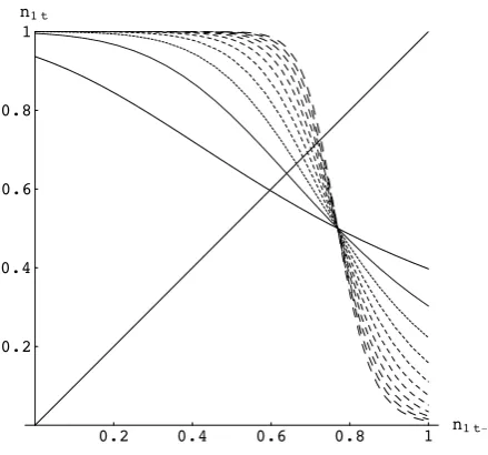
To show that our example actually has a steady state, we consider the function

Fβ,R(x) = nβ(x) + (1−nβ(x))x−Rx, where

nβ(x) = 1

1 + eβ(x−1)2.

IfFβ,R(x∗) = 0, then the price evolutionxt =x∗ for alltis a steady state equilibrium

of the dynamics in (28). We note that

Fβ,R(0) =nβ(0)>0,

Fβ,R(1/R) = nβ(1/R) + (1−nβ(1/R)) 1 R −1 = (1₋nβ(1/R))

!

−1 + 1 R

"

<0.

By the intermediate value theorem, there exists at least one x∗ ∈ (0,1/R) such

that F(x_∗) = 0. For either β > 0 sufficiently close to 0 or β sufficiently large, it

can be shown that this steady state equilibrium is actually unique; for intermediate

values ofβ, there may be several steady states. In fact, we can parametrize the steady

states as a function ofβ, by solving equation (29) forβ. This yields

β=β(x_∗) = 1

(1−x_∗)2log

1₋Rx_∗ (R−1)x_∗.

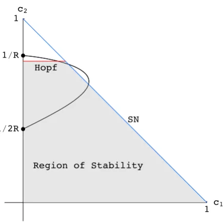
The graph of this function is illustrated in Figure 2. In appendix B it is shown that,

as the intensity of choiceβ increases, the following bifurcation scenario occurs. For

β = 0, the steady statex∗ = 1/(2R−1) = 1/(1 + 2r) ≈ 1(recall thatr =R−1).

Since we are working in scaled variables, this steady state is close toε, the predicted

steady state of type 1. Asβ increases, the steady statex_∗(β)moves along the upper

part of the curve in Figure 2, and this steady state is stable. Forβ = βSN1 ≈ 5.5two

additional steady states are created in a saddle-node bifurcation, one stable (the lower one) and one unstable (the middle one). Note that these two steady states are closer to

the fundamental valuex≡0. Asβincreases, the steady state closest to the

fundamen-tal values loses stability through a Hopf bifurcation atβHopf ≈11.0. AtβSN2 ≈13.6a

second saddle-node bifurcation occurs, and the two upper steady states disappear. For

βHopf <β < βSN2 a stable steady states co-exists with an attractor around the

(21)

5 10 15 Β

0 1!2R 1!R

x

SN1

SN2

[image:21.595.181.407.106.249.2]

Hopf

Figure 2: Steady state bifurcation diagram of the system(28) for R = 1.1 in scaled

coordinates. Values ofβare on the horizontal axis, values ofxon the vertical axis. The

curve shown is the locus of the steady state equilibriax∗. Note that there occur two saddle

node (SN) bifurcations and one Hopf bifurcation, and thatx∗→0, the true fundamental,

asβ → ∞. To obtain unscaled coordinates, multiply the values on the horizontal axis byε−2_{and those on the vertical axis by}_ε_.

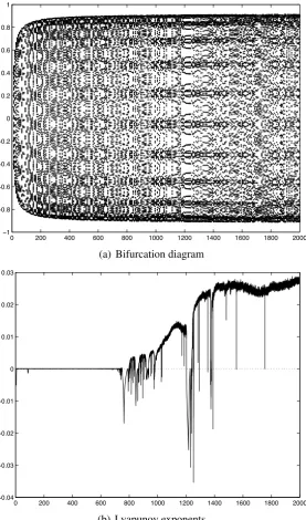
plot, illustrating the dynamical behavior after the Hopf bifurcation. After the Hopf

bifurcation (quasi-)periodic behavior occurs with a Lyapunov exponent close to0. For

large values of β the dynamics becomes chaotic, with positive Lyapunov exponent.

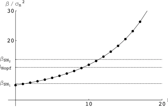
Introduction of additional Arrow securities has the same effect as increasing the

para-meterβ. For example, withS = 40 states of the world, all with equal probabilities

αi = 1/S, and dividendsyi =i−1, as in the previous example, fixingβ = 1yields the

following dynamics depending upon the numbernof Arrow securities (see Figure 4):

(i) unique stable steady state forn= 0andn= 1;

(ii) co-existence of two stable steady states for2_≤n_≤9;

(iii) co-existence of stable steady state and (quasi-)periodic attractor for n = 10

andn= 11;

(iv) (quasi-)periodic attractor, for12_≤n _≤32

(22)

0 200 400 600 800 1000 1200 1400 1600 1800 2000 !1

!0.8 !0.6 !0.4 !0.2 0 0.2 0.4 0.6 0.8 1

(a) Bifurcation diagram

0 200 400 600 800 1000 1200 1400 1600 1800 2000

!0.04

!0.03

!0.02

!0.01 0 0.01 0.02 0.03

[image:22.595.154.432.150.621.2]

(b) Lyapunov exponents

Figure 3:Bifurcation diagram (a) and Lyapunov exponent plot (b) of system(28)forR=

1.1,g = 1.101andε= 1in scaled coordinates. Values ofβ are on the horizontal axis,

values ofxand the first Lyapunov exponent are on the vertical axis in the upper and lower

(23)

10 20n Β_SN1

Β_Hopf Β_SN2

[image:23.595.156.427.110.289.2]

20 30 Β!Σ_n2

Figure 4:Plot of the coefficientβ(V−1

n )00 =β/(aσn2)as a function of the numbernof Arrow securities (scaled variables). There areS= 40states of the world, all with equal probabilitiesαi = 1/S, with dividendsyi = i−1. Other parameters areβ = 1and

R = 1.1. Without Arrow securities(V−1₎

00 = 1/(aσ2) = 1, but(Vn−1)00 = 1/(aσn2) increases as the number of Arrow securities increases and explodes whennapproaches

the number of statesS = 40. The first saddle node bifurcation value is crossed when the

number of Arrow securities increases from 1 to 2, the Hopf bifurcation value, where the system is destabilized, is crossed at the increase from 9 to 10, and the second saddle node value is crossed at the increase from 11 to 12.

3 Two period overlapping generations model

In this section we study reinforcement learning in a general equilibrium two period overlapping generations (OG) framework. OG models with adaptive learning have e.g. been studied by Grandmont (1985), Bullard (1994), Marcet and Sargent (1989), Sch¨onhofer (1999) and Bullard and Duffy (2001). A novel feature of this section is that we consider heterogeneous beliefs and investigate how Arrow securities affect the stability of the system. An earlier OG model with heterogeneous beliefs (but without Arrow securities) has been studied in Brock and DeFontnouvelle (2000).

3.1 Setup. Consider a world where agents live for two periods. They have

endow-mentsw1 andw2in their respective ‘young’ and ‘old’ periods. Their consumptionsc1

andc2 in these periods give them utility equal tou1(c1) +u2(c2). The functionsu1

andu2 are assumed to be continuous on [0,∞), (infinitely) differentiable on (0,∞),

monotonically increasing and to have a strictly negative second derivative everywhere; in particular, they are assumed to be strictly concave. Moreover, it is assumed that

u#

i(c)→ ∞asc→0fori= 1,2.

Young agents can consider to sell part of their endowment to the old agents living at the

same time, obtaining either a long–lived risky asset that pays an uncertain dividendys

in the next period, or an Arrow security for statei, payingδs

(24)

there areS states of the world andn Arrow securities,0 ≤ n < S. The price of the

consumptions good is normalized to 1. Young agents demand z0

t units of the risky

asset at the market pricep0

t, andzti units of thei’th Arrow security at pricepit, subject to their budget constraints

c1t+p0tzt0+#p˜t,z˜t$=w1, c2st =w2+ (p0t+1+ys)zt0+#δs,z˜t$,

where we use the same vector notationz˜t = (zt1,· · · , ztn) andp˜t = (p1t,· · · , pnt)as

before. The demandz0

t for the risky asset and z˜t for the Arrow security maximizes

their expected utility

Ut =u1(c1t) +Etu2(c2t)

=u1(w1−p0tzt0− #p˜t,z˜t$) +Etu2

#

w2+ (p0t+1+ys)zt0+#δs,z˜t$

$

.

Assumingu1 andu2to be strictly increasing smooth concave functions, utility is

max-imized whenever the derivatives ofUtwith respect to the demands vanish:

∂Ut

∂zt =

!

∂Ut

∂z0

t

,∂Ut ∂z˜t

"

= (0,0), (30)

where

∂Ut

∂z0

t

=₋u#₁.w1−p0tz0t − #p˜t,z˜t$

/

p0_t (31)

+Etu#2

.

w2+ (p0t+1+ys)zt0+#δs,z˜t$

/

(p0_t₊₁+ys),

and

∂Ut

∂z˜t

=−u#₁.w1−p0tz0t − #p˜t,z˜t$

/

˜

pt (32)

+Etu#2

.

w2+ (p0t+1+ys)zt0+#δs,z˜t$

/

δs.

3.2 Homogeneous agents. Total outside supply of the risky asset is assumed to be

constant through time; it is denoted byζ0_{. Total supply of each Arrow securities is}

zero, thus equilibrium prices are found by substituting

p0

t =p0∗, p˜t= ˜p∗, zt0 =ζ0, z˜t= 0, into equation (30), yielding

u#1(w1−p0_∗ζ0)p0_∗ = Etu#2

.

w2+ (p0_∗+ys)ζ0

/

(p0_∗+ys), (33)

pj

∗ =

u#₂.w2 + (p0_∗+yj)ζ0

/

u#

1(w1−p0_∗ζ0)

(25)

If there is a positive outside supply of risky assetsζ0 _> ₀_{, we can locate sufficient}

conditions for the existence of an equilibrium price. For, ifp0

∗ = 0, the left hand side

of (33) equals0while the right hand side of the same equation is positive. Likewise,

asp0

∗ →w1/ζ0, the left hand side increases beyond all positive bounds, while the right

hand side remains finite. By the intermediate value theorem, there is at least onep0

∗ >0

satisfying (33); we chose one of these, and we refer to it as the fundamental price of

the risky asset. Equation (34) then yields the corresponding fundamental pricesp˜_∗ of

the Arrow securities.

In the case of zero outside supply of risky assets, equations ((33)) and ((34)) can be solved for the fundamental prices

p0_∗ = Ey u#

1(w1)

u#

2(w2) −

1

and pj_∗ = u

#

2(w2)

u#

1(w1)

αj, j = 1,· · · , n.

To have a positive equilibrium price, it is sufficient to haveEy > 0 and u#

1(w1) >

u#₂(w2). These conditions are not directly obvious. However, ifu#1(w1)< u#2(w2), no

agent will want tosellthe risky asset, for his increase in utility in the first period will never be compensated by the decrease of utility in the second period, no matter how good the price. If the outside supply is non-zero, this argument does not hold since then all agents can hold a positive amount of the asset.

In general there will be multiple equilibria. Indeed there can even be an equilibrium price that is negative if limited liability does not hold. See Brock (1990) for discus-sion of the role of limited liability in eliminating negative price equilibria and how to construct examples of multiple equilibria.

In the special case of additively separable utility as in (33), differentiation with respect top0

∗ shows that the termu#1(w1−p0_∗ζ0)p_∗0 is increasing inp0_∗ ifu#1 >0,u##1 < 0. One

can also show that

∂ ∂p0

∗

.

Etu#2

#

w2+ (p0_∗+ys)ζ0

$

(p0_∗+ys)/ =Etu##2

#

w2+ (p0_∗+ys)ζ0

$

ζ0(p0_∗+ys) +Etu#2

#

w2+ (p0_∗+ys)ζ0

$

=Etu#2(cs2)

!

1 + c s

2u##2(cs2)

u#

2(cs2)

ζ0₍_p0

∗+ys) w2+ζ0(p0_∗ +ys)

"

,

wherecs

2 =w2+ (p0_∗+ys)ζ0. Notice that the sign of the last expression is the same as

the sign of the term in brackets sinceu#2 >0. Look at the casew2 = 0. The quantity

(1+cs

2u##2(cs2))/u#2(cs2)is just one minus the Arrow–Pratt relative risk aversion measure.

Thus, if the Arrow–Pratt relative risk aversion is always greater than one, forw2 = 0,

(26)

3.3 Heterogeneous agents. We are primarily interested in conditions for which the equilibrium found above is stable under reinforcement learning of heterogeneous agents, and how this stability depends on the number of Arrow securities. If prices are close to their equilibrium values, demands will be close to their respective

equilib-rium values. Demands are of the formz0

ht andz˜ht; they are combined in the demand vectorzht= (zht0 ,z˜ht). Also prices are collected in the price vectorpt= (p0t,p˜t). Heterogeneity is restricted to the agent’s expectation of the future price. As in section 2

we assume that an agent of typehexpects this to be

Ehtp0t+1 =p∗0+fht =p0ht+1.

As before,fh represents a function of past deviations from the fundamental according

to which typehbeliefs that prices will deviate from their fundamental benchmark.

3.3.1 Demands. We shall determine the demands of an agent of type h. Given a

price vector p, this agent determines his demands for the risky asset and the Arrow

securities by maximizing the utility function

Uht(zht) =u1(w1− #pt, zht$) +Ehtu2

#

w2+ (p0ht+1+ys)zht0 +#δs,z˜ht$

$

(35)

Denoting consumption of the agent in periodj withchj, the second order derivatives

of the functionU with respect tozread as

∂2_U

ht

∂(z0

ht)2

=u##₁(ch1)(p0t)2+Ehtu##2(csh2)(p0ht+1+ys)2,

∂2_U

ht

∂z0

ht∂z j ht

=u##₁(ch1)p0tp j

t+u##2(c

j h2)(p

0

ht+1+yj)αj,

∂2_U

ht

∂(z_htj )2 =u

##

1(ch1)(ptj)2+u##2(c

j h2)αj,

∂2_U

ht

∂z_htj ∂zk ht

=u##₁(ch1)pjtpkt, if k&=j.

In particular, the HessianHzhtUhtis negative definite; hence there is a unique demand

vectorzht=z(pt, p0ht+1)solving the maximization problem, which is differentiable as

a function ofpt.

3.3.2 Fitness. The average realized utilities uht+1 are obtained by replacing in the

expression (35) forUht idiosyncratic expectations p0ht+1 of the price of the risky

as-set by its realization p0

t+1, taking for the demands zt the realized demands zht and

averaging over all statess:

uht+1 =u1(w1− #pt, zht$) +Eu2

#

w2+ (p0t+1+y)zht0 +#δ,z˜ht$

$

(27)

Note that at the beginning of trading periodt, the most recent price known ispt−1, and

the most recent realized utility known isuht−1. This utility determines the fractionnht

of traders following type strategyhat the beginning of trading periodt, through

rein-forcement learning as discussed in Section 2:

nht = eβuht−1/Zt, Zt = H

*

h=1

eβuht−1_.

3.3.3 Prices. So far, we have determined demand and fitness of a trader of typeh.

Assume now that there areHtrader types in the market. Market clearing requires

H

*

h=1

nhtzht0 =ζ0, and

H

*

h=1

nhtz˜ht= 0, j = 1,· · · , n. (37)

There is a large literature on existence of equilibrium prices in incomplete markets; see e.g. Magill and Quinzii (1996) for an overview and the recent discussion in Cass (2006). However, most existence proofs are concerned with homogeneous expecta-tions. Heterogeneous expectations imply that the demands for Arrow securities may move differently for different trader types, which is an additional source of technical difficulties. For an existence proof taking heterogeneous characteristics into account see, e.g., Grandmont and Younes (1972). In order to be self-contained, in the appen-dix we demonstrate the existence of an equilibrium price vector for these markets with heterogeneous expectations; here we only give an outline of the argument.

LetP denote the set_{p_∈Rn+1_|_p

j >0forj = 0,1,· · · , n}of positive price vectors. We construct a homotopy of the problem from the homogeneous situation where all agents have the same expectations about future prices to the heterogeneous situation we are interested in. It is straightforward to show uniqueness and non-degenerateness of the price equilibrium in the homogeneous case.

We will construct a compact and convex subsetK _⊂P with piecewise smooth

bound-ary ∂K, which is such that along the homotopy, for every pt ∈ ∂K, the aggregate

excess demand vector z¯t(pt) = )hH=1nhtzht(pt) does not vanish. Then it follows

from topological arguments (index theory) that there is a price vectorpˆt ∈ K such

thatz¯t(ˆpt) = 0. The details of the proof can be found in section C of the appendix.

3.4 Dynamics close to a steady state equilibrium. We are mainly interested in the reinforcement learning dynamics within this general equilibrium OG framework. It turns out that a linear approximation of the learning dynamics around a homoge-neous steady state equilibrium has essentially the same structure as the evolutionary selection dynamics in the mean-variance asset pricing model with heterogeneous be-liefs in Section 2. This result can be derived under the general assumption that utility of agents of typehat timetis of the form