SFB
823
Minimum distance estimation
of Pickands dependence
function for multivariate
distributions
Discussion Paper
Betina Berghaus, Axel Bücher,
Holger Dette
Minimum distance estimation of Pickands dependence
function for multivariate distributions
Betina Berghaus, Axel B¨
ucher, Holger Dette
Ruhr-Universit¨
at Bochum
Fakult¨
at f¨
ur Mathematik
44780 Bochum, Germany
e-mail: [email protected] e-mail: [email protected] e-mail: [email protected]July 27, 2012
AbstractWe consider the problem of estimating the Pickands dependence function corresponding to a multivariate distribution. A minimum distance estimator is proposed which is based on a L2-distance between the logarithms of the empirical and an extreme-value copula. The mini-mizer can be expressed explicitly as a linear functional of the logarithm of the empirical copula and weak convergence of the corresponding process on the simplex is proved. In contrast to other procedures which have recently been proposed in the literature for the nonparamet-ric estimation of a multivariate Pickands dependence function [see Zhang et al. (2008) and Gudendorf and Segers (2011)], the estimators constructed in this paper do not require knowl-edge of the marginal distributions and are an alternative to the method which has recently been suggested by Gudendorf and Segers (2012). Moreover, the minimum distance approach allows the construction of a simple test for the hypothesis of a multivariate extreme-value copula, which is consistent against a broad class of alternatives. The finite-sample properties of the estimator and a multiplier bootstrap version of the test are investigated by means of a simulation study.
Keywords and Phrases: Extreme-value copula, minimum distance estimation, Pickands dependence function, weak convergence, copula process, test for extreme-value dependence
1
Introduction
Consider ad-dimensional random variableX = (X1, . . . , Xd) with continuous marginal distribution
functionsF1, . . . , Fd. It is well known that the dependency between the different components ofX
can be described in a margin-free way by the copula C, which is based on the representation
F(x1, . . . , xd) =C(F1(x1), . . . F(xd))
of the joint distribution functionF of the random vectorX[see Sklar (1959)]. A prominent class of copulas is the class of extreme-value copulas which arise naturally as the possible limits of copulas of component-wise maxima of independent, identically distributed or strongly mixing stationary sequences [see Deheuvels (1984) and Hsing (1989)]. For some applications of extreme-value copulas we refer to the work of Tawn (1988), Ghoudi et al. (1998), Coles et al. (1999) or Cebrian et al. (2003) among others.
A (d-dimensional) copula C is an extreme-value copula if and only if there exists a copula ˜C such that the relation
lim
n→∞
˜
C(u11/n, . . . , u1d/n)n=C(u1, . . . , ud) (1.1)
holds for all u = (u1, . . . , ud) ∈ [0,1]d. There exists an alternative description of multivariate
extreme-value copulas, which is based on a function on the simplex ∆d−1 := n t∈[0,1]d−1 d−1 X j=1 tj ≤1 o .
To be precise, a copula C is an extreme-value copula if and only if there exists a function A : ∆d−1 →[1/d,1] such that C has a representation of the form
C(u1, . . . , ud) = exp nXd j=1 loguj A logu2 Pd j=1loguj , . . . , logud Pd i=1loguj o . (1.2) The functionAis called Pickands dependence function [see Pickands (1981)]. If relation (1.2) holds true then the corresponding Pickands dependence function A is necessarily convex and satisfies the inequalities maxn1− d−1 X j=1 tj, t1, . . . , td−1 o ≤A(t)≤1
for all t = (t1, . . . , td−1) ∈ ∆d−1. In the case d = 2 these conditions are also sufficient for A to
be a Pickands dependence function. By the representation (1.2) of the extreme-value copula C
the problem of estimating C reduces to the estimation of the (d −1)-dimensional function A
and statistical inference for an extreme-value copula C may now be reduced to inference for its corresponding Pickands dependence function.
The problem of estimating Pickands dependence function nonparametrically has a long history. Early work dates back to Pickands (1981) and Deheuvels (1991). Alternative estimators have been proposed and investigated in the papers by Cap´era`a et al. (1997), Jim´enez et al. (2001), Hall and Tajvidi (2000), Segers (2007). These authors discuss the estimation of Pickands dependence function in the bivariate case and assume knowledge of the marginal distributions. Recently Genest and Segers (2009) and B¨ucher et al. (2011) proposed new estimators in the two-dimensional case which do not require this knowledge. While Genest and Segers (2009) considered rank-based versions of the estimators of Pickands (1981) and Cap´era`a et al. (1997), the approach of B¨ucher et al. (2011) is based on the minimum distance principle and yields an infinite class of estimators. The estimation problem of Pickands dependence function in the case d >2 was studied by Zhang et al. (2008) and Gudendorf and Segers (2011) assuming knowledge of the marginal distributions. Their estimators are based on functionals of the transformed random variablesYij =−logFj(Xij)
(i = 1, . . . , n , j = 1, . . . , d), which were also the basis for the estimators proposed by Pickands (1981) and Cap´era`a et al. (1997) in the bivariate case. Zhang et al. (2008) considered the random variable Zij(s) = V k:k6=j Yik sk Yij 1−sj + V k:k6=j Yik sk
where s= (s1, . . . , sd) such that (s2, . . . , sd)∈∆d−1 and s1 = 1−Pdj=2sj and Vj∈J aj = min{aj |
j ∈ J }. They showed that the corresponding distribution function depends in a simple way on a partial derivative of the logarithm of Pickands dependence function and proposed to estimate Pickands dependence function by using a functional of the empirical distribution function of the random variables Zij(s). The obtained estimator is uniformly consistent and converges point-wise
to a normal distribution.
Gudendorf and Segers (2011) discussed the random variable ξi(s) = Vdj=1Ysij
j which is
Gumbel-distributed with location parameter logA(s2, . . . , sd). They suggested to estimate Pickands
de-pendence function by the method-of-moments and also provided an endpoint correction to impose (some of) the properties of Pickands dependence function. They also discussed the asymptotic properties of the estimator and a way to get optimal weight functions needed in the endpoint cor-rections. It was shown that the least squares estimator leads to weight functions which minimize the asymptotic variance. Furthermore, Gudendorf and Segers (2011) showed that in some cases their estimator coincides with the one proposed by Zhang et al. (2008). Recently, Gudendorf and Segers (2012) extended this methodology of Gudendorf and Segers (2011) to the case of unknown marginals.
The present paper is devoted to the construction of an alternative class of estimators of Pickands dependence function in the general multivariate cased≥2, which also do not require knowledge of the marginal distribution. For this purpose we will use the minimum distance approach proposed
in B¨ucher et al. (2011), which allows us to construct an infinite dimensional class of estimators, which depend in a linear way on the logarithm of the d-dimensional empirical copula. Because this statistic does not require knowledge of the marginals the resulting estimator of Pickands dependence function does automatically not depend on the marginal distributions of X. We also briefly discuss the properties of our methods in the case of dependent data.
Moreover, the minimum distance approach also allows us to construct a simple test for the hypoth-esis that a given copula is an extreme-value copula. In this case the distance between the copula and its best approximation by an extreme-value copula is 0, and as a consequence a consistent estimator of the minimum distance should be small. Therefore the hypothesis of an extreme-value copula can be rejected for large values of this estimator. A multiplier bootstrap for the approx-imation of the critical values is proposed and its consistency proved. Moreover, we demonstrate that the new bootstrap is also applicable in the context of dependent data. Alternative tests for extreme-value dependence in dimension d >2 in the case of independent data have recently been proposed by Kojadinovic et al. (2011) [for tests in dimension d= 2 for independent data see, e.g., Ghoudi et al. (1998); Ben Ghorbal et al. (2009); Kojadinovic and Yan (2010); B¨ucher et al. (2011); Genest et al. (2011); Quessy (2011)].
The remaining part of the paper is organized as follows. In Section 2 we present the necessary notation and define the class of minimum distance estimators. The main asymptotic properties are given in Section 3, while the corresponding test for the hypothesis of an extreme value copula is investigated in Section 4. Here we also establish consistency of the multiplier bootstrap such that critical values can easily be calculated by numerical simulation. The finite-sample properties of the new estimators and the test are investigated in Section 5, where we also present a brief comparison with the estimators proposed by Gudendorf and Segers (2012). Finally some technical details are deferred to an Appendix in Section 5.
2
Measuring deviations from an extreme-value copula
Throughout this paper we define A as the set of all functions A : ∆d−1 → [1/d,1] and Π is the
independence copula, that is Π (u1, . . . , ud) =
Qd
j=1uj. For most statements in this paper we
will assume that the copula C satisfies C ≥ Π (or a slight modification of this statement). This assumption is equivalent to positive quadrant dependence of the random variables, that is for every (x1, . . . , xd)∈Rd we have P(X1 ≤x1, . . . , Xd≤xd)≥ d Y j=1 P(Xj ≤xj).
Obviously it holds for any extreme-value copula because of the lower bound of Pickands dependence function. Following B¨ucher et al. (2011) the construction of minimum distance estimators for
Pickands dependence function is based on a weighted L2-distance Mh(C, A) = Z (0,1)×∆d−1 logC y1−t1−...−td−1, yt1, . . . , ytd−1−log (y)A(t) 2h(y)d(y,t), (2.1)
where h : [0,1] → R+ is a continuous weight function and t = (t
1, . . . , td−1) ∈ ∆d−1. The result
below gives an explicit expression of the best L2-approximation of the logarithm of a copula
satisfying this condition.
Theorem 2.1. Assume that the copula C satisfies C ≥ Πκ for some κ ≥ 1 and that the weight function h satisfiesR01(logy)2h(y)dy <∞. Then
A∗ = argmin{Mh(C, A)|A∈ A}
is well-defined and given by A∗(t) =Bh−1 Z 1 0 logC(y1−t1−...−td−1, yt1, . . . , ytd−1) logy h ∗ (y)dy, (2.2)
where we use the notations
h∗(y) = log2(y)h(y) (2.3) and Bh = R1 0 (logy) 2 h(y)dy =R1 0 h
∗(y)dy . Moreover, if C ≥Π, the function A∗ defined in (2.2)
satisfies maxn1− d−1 X j=1 tj, t1, . . . , td−1 o ≤A∗(t)≤1.
Proof. Since C ≥Πκ we obtain
1≥C y1−t1−...−td−1, yt1, . . . , ytd−1 ≥Π y1−t1−...−td−1, yt1, . . . , ytd−1κ =yκ
and thus
0≥log C y1−t1−...−td−1, yt1, . . . , ytd−1 ≥κlogy.
This yields|logC(y1−t1−...−td−1, yt1, . . . , ytd−1)| ≤κ|logy|and therefore the integral in (2.2) exists.
By Fubini’s theorem the weighted L2-distance can be rewritten as
Mh(C, A) = Z ∆d−1 Z 1 0 logC(y1−t1−...−td−1, yt1, . . . , ytd−1) logy −A(t) 2 log2(y)h(y) dy dt,
and now the first part of the assertion is obvious.
For a proof of the second part we make use of the upper Fr´echet-Hoeffding-bound and obtain
A∗(t)≥Bh−1 Z 1 0 log min{y1−t1−...−td−1, yt1, . . . , ytd−1} logy h ∗ (y)dy
=Bh−1 Z 1 0 maxn1− d−1 X j=1 tj, t1, . . . , td−1 o h∗(y)dy = maxn1− d−1 X j=1 tj, t1, . . . , td−1 o .
With a similar calculation and the assumption C ≥Π we obtain the upper bound.
A possible choice for the weight function is given by h(y) = −yk/logy, where k ≥0, see Example
2.5 in B¨ucher et al. (2011). In Section 5 we consider this weight function with k = 0.5.
If the copula C is not an extreme-value copula the function A∗ has not necessarily to be convex for any copula satisfying C ≥ Π [see B¨ucher et al. (2011)]. However, for every copula satisfying
C ≥ Πκ for some κ ≥ 1 the equality M
h(C, A∗) = 0 holds if and only if the copula C is an
extreme-value copula with Pickands dependence function A∗. This property will be useful for the construction of a test for the hypothesis thatCis an extreme-value copula, which will be discussed in Section 4. For this purpose we will need an empirical analogue of the “best approximation” A∗
which is constructed and investigated in the following section.
3
Weak convergence of minimal distance estimators
Throughout the remaining part of this paper let X1, . . . ,Xn denote independent identically
dis-tributed Rd-valued random variables. We define the components of each observation by X i =
(Xi1, . . . , Xid) (i= 1, . . . , n) and assume that all marginal distribution functions of Xi are
contin-uous. The copula of Xi can easily be estimated in a nonparametric way by the empirical copula
[see, e.g., R¨uschendorf (1976)] which is defined for u= (u1, . . . , ud) by
Cn(u) = 1 n n X i=1 I{Uˆi1 ≤u1, . . .Uˆid≤ud}, (3.1) where ˆUij = n+11 Pn
k=1I{Xkj ≤ Xij} denote the normalized ranks of Xij amongst X1j, . . . , Xnj.
Following B¨ucher et al. (2011) we use Theorem 2.1 to construct an infinite class of estimators for Pickands dependence function by replacing the unknown copula with the empirical copula. To avoid zero in the logarithm we use a modification of the empirical copula. We set ˜Cn=Cn∨n−γ
where γ > 12 and obtain the estimator
b An,h(t) = Bh−1 Z 1 0 log ˜Cn(y1−t1−...−td−1, yt1, . . . , ytd−1) logy h ∗ (y)dy. (3.2) The weak convergence of the empirical process√n(Cn−C) was investigated by R¨uschendorf (1976)
and Fermanian et al. (2004) among others under various assumptions on the partial derivatives of the copulaC. Recently Segers (2012) proved the weak convergence of the empirical copula process
Cn=
√
n(Cn−C) GC in (`∞[0,1] d
under a rather weak assumption, which is satisfied for many copulas, that is
∂jC(u) exists and is continuous on {u∈[0,1] d
|uj ∈(0,1)} (3.4)
for every j = 1, . . . , d. The limiting process GC in (3.3) depends on the unknown copula and is
given by GC(u) = BC(u)− d X j=1 ∂jC(u)BC(1, . . . ,1, uj,1, . . . ,1), (3.5)
where we set ∂jC(u) = 0, j = 1, . . . , d for the boundary points {u ∈ [0,1] d
| uj ∈ {0,1}}. Here,
BC is a centered Gaussian field on [0,1]d with covariance structure
r(u,v) = Cov (BC(u),BC(v)) = C(u∧v)−C(u)C(v),
and the minimum is understood component-wise. Note that it can be shown that (3.4) holds for any extreme-value copula with continuously differentiable Pickands dependence function. The following result describes the asymptotic properties of the new estimators Abn,h for Pickands dependence
function. Weak convergence takes place in the space of all bounded functions on the unit simplex ∆d−1, equipped with the topology induced by the sup-norm k · k∞. The proof is given in the
Appendix.
Theorem 3.1. If the copula C ≥Π satisfies condition (3.4), and the weight functionh∗ satisfies
h∗ log ∞ <∞ and Z 1 0 h∗(y) (−logy)−1y−λdy <∞ (3.6)
for some λ >1, then we have for any γ ∈ 1 2, λ 2 as n → ∞ √ n(Abn,h−A∗) AC,h (3.7)
in `∞(∆d−1), where the limiting process is defined by
AC,h =Bh−1 Z 1 0 GC(y1−t1−...−td−1, yt1, . . . , ytd−1) C(y1−t1−...−td−1, yt1, . . . , ytd−1) h∗(y) logy dy.
Remark 3.2. A careful inspection of the proof of this result shows that weak convergence of the empirical copula process lies at the heart of its proof. Since the latter converges under fairly more general conditions on the serial dependence of a stationary time series, the i.i.d. assumption on the series X1, . . . ,Xn can be easily dropped. Exploiting the results in B¨ucher and Volgushev (2011),
the assertion of Theorem 3.1 holds true for every stationary sequence of random vectors provided Condition 2.1 in that reference is met. This condition is so mild that all usual concepts of weak serial dependence are included, e.g., strong mixing or absolute regularity of a time series at a mild
polynomial decay of the corresponding coefficients. For details we refer to B¨ucher and Volgushev (2011). The only difference to the i.i.d. case is reflected in a differing asymptotic covariance of the process BC which is now given by
Cov(BC(u),BC(v)) =
X
j∈Z
Cov(I{U0 ≤u},I{Uj ≤v}),
and which, of course, reduces to C(u∧v)−C(u)C(v) in the i.i.d. setting.
Note that the result of Theorem 3.1 is correct even in the case where C is not an extreme-value copula because the centering in (3.7) uses the best approximation with respect to the L2 -distance. The discussed estimator Abn,h in general will neither be convex nor will it necessarily
satisfy the boundary conditions of a multivariate Pickands dependence function. To ensure the latter restriction, one can replace the estimator ˆAn,h by the statistic
maxn1− d−1 X j=1 tj, t1, . . . td−1,min{Aˆn,h(t),1} o .
Furthermore, to provide convexity, the greatest convex minorant of this statistics can be used. As a consequence the estimator Abn,h is replaced by a convex estimator with a smaller sup-norm
between the true Pickands dependence function and the corresponding estimator, see Wang (1986). An alternative way to achieve convexity and to correct for boundary properties of Abn,h is the
calculation of theL2-projection on the space of partially linear functions satisfying these properties.
This proposal was investigated by Fils-Villetard et al. (2008) and decreases theL2-distance instead
of the sup-norm.
Finally, we would like to point that none of these procedures guarantee that the modified estimator is in fact a Pickands dependence function, because these properties do not characterize Pickands dependence function in the case d≥3.
4
A test for extreme-value dependence
To construct a test for extreme-value dependence we reconsider theL2-distanceMh(C, A∗) defined
in (2.1). The following result will motivate the choice of the test statistic.
Lemma 4.1. If h is a strictly positive weight function with h∗ ∈L1(0,1), then C ≥Πκ for some
κ≥1 is an extreme-value copula if and only if
min{Mh(C, A)|A∈ A}=Mh(C, A∗) = 0.
Proof. If C is an extreme-value copula then A∗ is the Pickands dependence function of the copula C and the weighted L2-distance is equal to 0.
Now assume Mh(C, A∗) = 0. With the definition of theL2-distance we obtain
logC(y1−t1−...−td−1, yt1, . . . , ytd−1) = log(y)A∗(t)
almost surely with respect to the Lebesgue measure on the set (0,1)×∆d−1. Since the functions
logC(y1−t1−...−td−1, yt1, . . . , ytd−1) and (logy)A∗(t) are continuous functions, the equality holds on
the whole domain. This yields with a transformation for every u1, . . . , ud∈(0,1]
C(u1, . . . , ud) = exp nXd j=1 loguj A∗ logu2 Pd j=1loguj , . . . logud Pd i=1loguj o .
and it can easily be shown that this identity also holds on the boundary. As a consequence, C is max-stable and thus an extreme-value copula.
Lemma 4.1 suggests to use Mh( ˜Cn,Aˆn,h) as a test statistic for the hypothesis
H0 : C is an extreme-value copula (4.1)
and to reject the null hypothesis for large values of Mh( ˜Cn,Aˆn,h). We now will investigate the
asymptotic distribution of the test statistic under the null hypothesis and the alternative.
Theorem 4.2. Let C be an extreme-value copula satisfying condition (3.4) with Pickands depen-dence function A. If the weight function h is strictly positive, satisfies (3.6) and additionally the conditions khk∞<∞ and Z 1 0 h(y) yλ dy <∞ (4.2)
hold for some λ >2, then we have for any γ ∈ 1 2, λ 4 as n→ ∞ nMh( ˜Cn,Aˆn,h) Z0,
where the random variable Z0 is defined by
Z0 := Z ∆d−1 Z 1 0 GC(y1−t1−...−td−1, yt1, . . . , ytd−1) C(y1−t1−...−td−1, yt1, . . . , ytd−1) 2 h(y)dy dt−Bh Z ∆d−1 A2C,h(t)dt,
and the constant Bh and the process AC,h are defined in Theorem 3.1.
The following result will give the asymptotic distribution of the test statistic under the alternative. Note that this is the case if and only if Mh(C, A∗)>0.
Theorem 4.3. LetC ≥Π be a copula satisfying condition (3.4) such that Mh(C, A∗)>0 . If the
strictly positive weight function h and the function h∗ defined in (2.3) satisfy the conditions (3.6) and (4.2) for some λ >1, then we have for any γ ∈(12,1+4λ ∧ λ
2) as n→ ∞
√
Here the random variable Z1 is defined by Z1 := 2 Z ∆d−1 Z 1 0 GC(y1−t1−...−td−1, yt1, . . . , ytd−1) C(y1−t1−...−td−1, yt1, . . . , ytd−1) ν(y,t) dy dt
with weight function
ν(y,t) = nlogC(y1−Pdi=1−1ti, yt1, . . . , ytd−1)−log(y)A∗(t)
o
h(y).
Remark 4.4.
a) Again, the i.i.d. assumption onX1, . . . ,Xn in both preceding Theorems can be relaxed to weak
serial dependence and strong stationarity, see Remark 3.2 above.
b) From Theorem 4.2 and 4.3 we obtain an asymptotic level α test for the hypothesis (4.1) by rejecting the null hypothesis H0 if
nMh( ˜Cn,Aˆn,h)> z1−α,
wherez1−αdenotes the (1−α)-quantile of the distribution of the random variableZ0. By Lemma 4.1
and Theorem 4.3 the test is (at least) consistent against all alternatives C≥Π satisfying assump-tion (3.4).
c) Note that the random variable Z1 in Theorem 4.3 is normal distributed, with mean 0 and
variance, say σ2. Consequently the power of the test is approximately given by
P(nMh( ˜Cn,Aˆn,h)> z1−α) ≈ 1−Φ z1−α √ nσ − √ nMh(C, A ∗) σ ≈Φ√nMh(C, A ∗) σ ,
where A∗ is defined in (2.2) and Φ denotes the standard normal distribution function. Thus the power of the test is an increasing function with respect to n depending on the quantity Mh(C,A∗)
σ ,
see B¨ucher et al. (2011).
For the construction of the test we need the (1−α)-quantile of the distribution of the random variable Z0. Unfortunately, this distribution depends on the unknown copula C and therefore it
cannot be explicitly determined. However, we can easily construct a test if we approximate the distribution of the random variable Z0 by the multiplier bootstrap [see R´emillard and Scaillet
(2009), B¨ucher and Dette (2010) and Segers (2012)].
To this end, let ∂[jCn(u) be an estimator for ∂jC(u) which is uniformly bounded in n and u and
for any δ ∈(0,1/2) satisfies the condition sup
u∈[0,1]d:uj∈[δ,1−δ]
as n → ∞. It is easily seen, that for instance the following estimator based on finite differencing of the empirical copula satisfies these conditions:
[ ∂jCn(u) = Cn(u+hnej)−Cn(u−hnej) 2hn if uj ∈[hn,1−hn] [ ∂jCn(u1, . . . , uj−1, hn, uj+1, . . . , ud) if uj ∈[0, hn) [ ∂jCn(u1, . . . , uj−1,1−hn, uj+1, . . . , ud) if uj ∈(1−hn,1],
where hn → 0 is a bandwidth such that infnhn
√
n > 0 and where ej denotes the jth unit vector
in Rd.
Now, let ξ1, ξ2, ... denote independent identically distributed random variables with mean 0 and
variance 1 independent fromX1,X2, ...satisfying
R∞ 0 p P (|ξ1|> x)dx <∞. Define αξn(u) = √1 n n X i=1 ξi n I{Uˆi,1 ≤u1, . . . ,Uˆi,d ≤ud} −Cn(u) o and set Cξn(u) =α ξ n(u)− d X j=1 [ ∂jCn(u)αξn(1, . . . ,1, uj,1, . . . ,1).
It follows from the results in Segers (2012) that if C satisfies condition (3.4), then (Cn,Cξn) (GC,G
0
C)
in (`[0,1]d,k · k∞)2, whereGC denotes the process defined in (3.5) and G
0
C is an independent copy
of this process. By the results in B¨ucher and Ruppert (2012) we also obtain conditional weak convergence of Cξn given the data in probability, which we denote by
Cξn
P
ξ GC.
For details on that type of convergence we refer to the monograph Kosorok (2008). Our final result now shows that the multiplier bootstrap procedure can be used to obtain a valid approximation for the distribution of the random variable Z0.
Theorem 4.5. Assume the Copula C ≥ Π satisfies condition (3.4). If the weight function h satisfies the conditions in Theorem 4.2 and the functiony 7→h∗(y)(ylogy)−2 is uniformly bounded, then we get for the random variable
ˆ Zn = Z ∆d−1 Z 1 0 Cξn(y1−t1−...−td−1, yt1, . . . , ytd−1) ˜ Cn(y1−t1−...−td−1, yt1, . . . , ytd−1) 2 h(y)dy dt −Bh−1 Z ∆d−1 Z 1 0 Cξn(y1−t1−...−td−1, yt1, . . . , ytd−1) ˜ Cn(y1−t1−...−td−1, yt1, . . . , ytd−1) h∗(y) logydy 2 dt
the weak conditional convergence Zˆn P ξ Z0.
Proof. Due to the assumptions on the weight function all integrals in the definition of Z0 are
proper and therefore the mapping (GC, C) 7→ Z0(GC, C) is continuous. Hence, the result follows
from Cξn P
ξ GC and the continuous mapping theorem for the bootstrap, see, e.g., Theorem 10.8
in Kosorok (2008).
The bootstrap test is now obtained as follows. Repeating the procedure B times yields a sample ˆ
Zn(1), . . . ,Zˆn(B) that is approximately distributed according to Z0. This suggests to reject the
null hypothesis if
nMh( ˜Cn,Aˆn,h)>zˆ1−α,
where ˆz1−α denotes the empirical (1−α)-quantile of this sample. It follows from Theorem 4.5 that
the test holds its level α asymptotically and that it is consistent. The finite-sample performance of the test is investigated in the following section.
Remark 4.6. By the results in B¨ucher and Ruppert (2012) a block multiplier bootstrap can be used to obtain a valid bootstrap approximation of Z0 in the case of strongly mixing stationary
time series. We omit the details for the sake of brevity.
5
Finite-sample properties
This section is devoted to a simulation study regarding the finite-sample properties of the proposed estimators and tests for extreme-value copulas. We begin our discussion with the performance of the estimators. For that purpose we consider the trivariate extreme-value copula of logistic type as presented in Tawn (1990) with Pickands dependence function defined for t= (t1, t2)∈∆2 by
A(t) = (θ1/αs11/α+φ1/αs12/α)α+ (θ1/αs21/α+φ1/αs13/α)α+ (θ1/αs13/α+φ1/αs11/α)α +ψ(s11/α+s12/α+s13/α)α+ 1−θ−φ−ψ,
where s = (s1, s2, s3) := (1 −t1 − t2, t1, t2) and (α, θ, φ, ψ) ∈ (0,1]× [0,1]3. For the sake of
comparison with existing simulation studies in the literature [see Gudendorf and Segers (2012)] we considered the parameters (θ, φ, ψ) = (0,0,1) corresponding to a symmetric copula model (also widely known as the Gumbel–Hougaard copula) and (θ, φ, ψ) = (0.6,0.3,0) corresponding to an asymmetric logistic copula. The parameter α was chosen from the set {0.3,0.5,0.7,0.9}.
Regarding the choice of the weight function we followed the proposal in B¨ucher et al. (2011) and considered the function h(y) = −yk/log(y) with k = 0.5. This choice seems to be a good
compromise between a possibly difficult data-adaptive way of choosing a weight function and anaytical tractability, see Section 3.7 in B¨ucher et al. (2011). Additional simulations in dimension
in the two-dimensional study in the last-named reference. Furthermore, we refer to Section 3.4 in B¨ucher et al. (2011) for a discussion of “optimal” weight functions.
In Tables 1 and 2 we report Monte-Carlo approximations for the mean integrated squared error (MISE)E[R( ˆA−A)2] for the multivariate CFG-estimator, Pickands estimator (see Gudendorf and Segers (2012)) and the estimator introduced in the present paper which we abbreviate by BDV according to B¨ucher et al. (2011). All estimators are corrected for the boundary conditions on Pickands dependence function. The BDV-estimator is replaced by the function
maxn1− d−1 X j=1 tj, t1, . . . td−1,min{Aˆn,h(t),1} o .
For the Pickands- and CFG-estimator we used the endpoint-corrections supposed in Gudendorf and Segers (2012). For each scenario we simulated 1.000 samples of size n ∈ {50,100,200}
using the simulation algorithms in Stephenson (2003) which are implemented in the R-package
evd, Stephenson (2002). The main finings are as follows.
• The Pickands estimator is outperformed by the CFG and the BDV estimator. Regarding only the former two estimators this finding is in-line with the simulation study in Gudendorf and Segers (2012).
• The CFG and the BDV estimator yield comparable results with slight advantages for the CFG estimator for strong dependence, whereas weak dependence results in more efficiency for the BDV estimator.
[Insert Tables 1 and 2 about here]
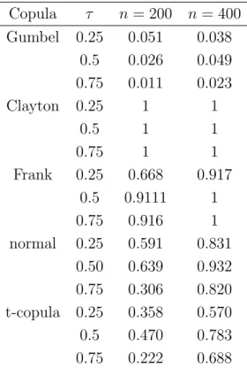
Finally, we conducted Monte Carlo experiments to investigate the level and the power of the test for extreme-value dependence introduced in Section 4. We fixed the dimension to d = 3 and considered samples of sizen= 200 andn= 400 where the level of the test isα = 5%. Under the null hypothesis we simulated from the symmetric logistic type model as defined in (6.1) with parameters (θ, φ, ψ) = (0,0,1) (i.e., the Gumbel–Hougaard copula). For the sake of a comparison with the two-dimensional version of the test in B¨ucher et al. (2011) and with the extensive simulation study in Kojadinovic et al. (2011) we chose the remaining parameter α in such a way that Kendall’s tau varies in the set{0.25,0.5,0.75}. Under the alternative we considered the Clayton, Frank, Normal andt-copula with four degrees of freedom and the same values for Kendall’s tau. For the multiplier method we chose B = 100 Bootstrap-replicates. The test was carried out at the 5% significance level and empirical rejection rates were computed from 1.000 random samples in each scenario. The results are stated in Table 3. The main findings are as follows.
• The test seems to be globally too conservative, although the observed level improves with increasing sample size. This effect is observed to be stronger for increasing level of dependence
(measured by Kendall’s tau) and is in-line with other simulation studies on the multiplier method for copulas with strong dependence.
• In terms of power the test detects all alternatives with reasonable rejection rates. Clayton and Frank’s copula are detected more often, as it was supposed to under consideration of the findings in B¨ucher et al. (2011).
[Insert Table 3 about here]
Acknowledgements. This work has been supported by the Collaborative Research Center “Sta-tistical modeling of nonlinear dynamic processes” (SFB 823, Teilprojekt A1, C1) of the German Research Foundation (DFG). The authors are grateful to Stanislav Volgushev for discussions and suggestions concerning this manuscript. Parts of this paper were written while H. Dette was visit-ing the Institute of Mathematical Sciences at the National University of Svisit-ingapore and this author would like to thank the institute for its hospitality.
6
Proofs
6.1
Proof of Theorem 3.1
The proof follows from a slightly more general result, which establishes weak convergence for the weighted process Wn,ω(t) = Z 1 0 log ˜ Cn(y1−t1−...−td−1, yt1, . . . , ytd−1) C(y1−t1−...−td−1, yt1, . . . , ytd−1)ω(y,t)dy, (6.1)
where the weight function ω : [0,1]× ∆d−1 may depend on y and t. Theorem 3.1 is a simple
consequence of the following result using the weight function ω(y,t) = Bh−1hlog∗(yy) which does not depend on t.
Theorem 6.1. Assume that for the weight function ω : [0,1]×∆d−1 →R there exists a bounded
function ω : [0,1] → R0+ such that |ω(y,t)| ≤ ω(y) for all y ∈ [0,1] and all t ∈ ∆d−1 and such
that
Z 1
0
ω(y)y−λdy <∞ for some λ >1. (6.2)
If the copula C ≥Π satisfies (3.4) then we have for every γ ∈ 1
2, λ 2 as n→ ∞ √ nWn,ω(t) WC,ω(t) in `∞(∆d−1),
where the limiting process is given by WC,ω(t) = Z 1 0 GC(y1−t1−...−td−1, yt1, . . . , ytd−1) C(y1−t1−...−td−1, yt1, . . . , ytd−1) ω(y,t)dy.
Proof of Theorem 6.1. Fix λ >1 andγ ∈ 1 2,
λ
2
. Due to Lemma 1.10.2 in Van der Vaart and Wellner (1996), the processes √n( ˜Cn−C) and
√
n(Cn−C) will have the same weak limit.
For i= 1,2, ...we consider the following random functions in `∞(∆d−1) :
Wn(t) := Z 1 0 √ nlog ˜Cn(y1−t1−...−td−1, yt1, . . . , ytd−1) −logC(y1−t1−...−td−1, yt1, . . . , ytd−1) ω(y,t)dy Wi,n(t) := Z 1 1/i √ n log ˜Cn(y1−t1−...−td−1, yt1, . . . , ytd−1) −logC(y1−t1−...−td−1, yt1, . . . , ytd−1) ω(y,t)dy W(t) := Z 1 0 GC(y1−t1−...−td−1, yt1, . . . , ytd−1) C(y1−t1−...−td−1, yt1, . . . , ytd−1) ω(y,t)dy Wi(t) := Z 1 1/i GC(y1−t1−...−td−1, yt1, . . . , ytd−1) C(y1−t1−...−td−1, yt1, . . . , ytd−1) ω(y,t)dy
With this notation we have to show the following three assertions : (i) Wi,n Wi in`∞(∆d−1) forn → ∞,
(ii) Wi W in`∞(∆d−1) for i→ ∞,
(iii) for every ε >0: limi→∞limn→∞P∗
supt∈∆d−1|Wi,n(t)−Wn(t)|> ε
= 0,
then Lemma B.1 in B¨ucher et al. (2011) yields the convergenceWn W in`∞(∆d−1).
We begin with the proof of assertion (i). For this purpose we set Ti = [1/i,1] d
for i ∈ N and consider the mapping
Φ1 : DΦ1 →` ∞(T i) f 7→log◦f,
where the domain is defined by DΦ1 := {f ∈ `
∞(T
i) | infx∈Ti|f(x)| > 0}. Due to Lemma 12.2
in Kosorok (2008), it follows that Φ1 is Hadamard-differentiable at C tangentially to `∞(Ti) with
derivative Φ01,C(f) = Cf. Since ˜Cn≥n−γ andC ≥Π, we have ˜Cn,C ∈DΦ1 and with the functional
delta method we obtain
√
n(log ˜Cn−logC) G C
for n→ ∞ in `∞(Ti). Now we consider the mapping Φ2 : `∞(Ti)→`∞([1/i,1]×∆d−1) f 7→f ◦φ ,
where the mapping φ : [1/i,1]×∆d−1 →Ti is defined by
φ(y,t) = (y1−t1−...−td−1, yt1, . . . , ytd−1).
For Φ2 the following inequality holds:
kΦ2(f)−Φ2(g)k∞= sup y∈[1/i,1],t∈∆d−1 |f◦φ(y,t)−g◦φ(y,t)| ≤ sup x∈Ti |f(x)−g(x)|=kf −gk∞.
This implies that Φ2 is Lipschitz-continuous. By the continuous mapping theorem and the
bound-edness of the weight function ω we obtain
√ nnlog ˜Cn(y1−t1−...−td−1, yt1, . . . , ytd−1)−logC(y1−t1−...−td−1, yt1, . . . , ytd−1) o ω(y,t) GC(y1−t1−...−td−1, yt1, . . . , ytd−1) C(y1−t1−...−td−1, yt1, . . . , ytd−1) ω(y,t) in `∞ [1i,1]×∆d−1
. By integration with respect to y∈[1/i,1] assertion (i) follows.
Assertion (ii) follows directly from the observation, that the process GC is bounded on [0,1] d
and from the fact, that the function
t7→ ω(y,t)
C(y1−t1−...−td−1, yt1, . . . , ytd−1)
can be bounded by the integrable function ω(y)y−1. The proof of (iii) is obtained by the same
arguments as given in B¨ucher et al. (2011) in the case d= 2 and is therefore omitted.
6.2
Proof of Theorem 4.2
Since integration is continuous, it suffices to show the weak convergence ¯Wn(t) W¯ (t) in
`∞(∆d−1), where we define ¯ Wn(t) = Z 1 0 n log ˜ Cn(y1−t1−...−td−1, yt1, . . . , ytd−1) C(y1−t1−...−td−1, yt1, . . . , ytd−1) !2 h(y)dy−nBh( ˆAn,h(t)−A(t))2 ¯ W(t) = Z 1 0 GC(y1−t1−...−td−1, yt1, . . . , ytd−1) C(y1−t1−...−td−1, yt1, . . . , ytd−1) !2 h(y)dy−BhA2C,h(t).
Now we will proceed similar to the proof of Theorem 6.1 and consider ¯ Wi,n(t) = Z 1 1/i n logC˜n(y 1−t1−...−td−1, yt1, . . . , ytd−1) C(y1−t1−...−td−1, yt1, . . . , ytd−1) !2 h(y)dy −Bh−1 Z 1 1/i √ nlog ˜ Cn(y1−t1−...−td−1, yt1, . . . , ytd−1) C(y1−t1−...−td−1, yt1, . . . , ytd−1) h∗(y) logy dy !2 ¯ Wi(t) = Z 1 1/i GC(y1−t1−...−td−1, yt1, . . . , ytd−1) C(y1−t1−...−td−1, yt1, . . . , ytd−1) !2 h(y)dy −Bh−1 Z 1 1/i GC(y1−t1−...−td−1, yt1, . . . , ytd−1) C(y1−t1−...−td−1, yt1, . . . , ytd−1) h∗(y) logy dy !2 .
Due to Lemma B.1 in B¨ucher et al. (2011) it suffices to show (i) ¯Wi,n W¯i in`∞(∆d−1) for n→ ∞,
(ii) ¯Wi W¯ in`∞(∆d−1) for i→ ∞,
(iii) for every ε >0: limi→∞limn→∞P∗
supt∈∆ d−1| ¯ Wi,n(t)−W¯n(t)|> ε = 0.
The proof of these assertions follows by similar arguments as in B¨ucher et al. (2011) and is omitted for the sake of brevity.
6.3
Proof of Theorem 4.3
We use the decomposition
Mh( ˜Cn,Aˆn,h)−Mh(C, A∗) = S1+S2+S3, (6.3) where S1 = 2 Z ∆d−1 Z 1 0 ¯ Cn(y,t)−C¯(y,t) ¯ C(y,t)−A∗(t) (−logy) h(y)dy dt, S2 = Z ∆d−1 Z 1 0 ¯ Cn(y,t)−C¯(y,t) 2 h(y)dy dt S3 =−Bh Z ∆d−1 n ˆ An,h(t)−A∗(t) o2 dt
and we used the notations ¯
C(y,t) =−logC(y1−t1−...−td−1, yt1, . . . , ytd−1),
¯
To investigate the convergence of the first term in (6.3) we first notice that |ν(y,t)| ≤ν¯(y), with ¯
ν(y) := −2hlog∗(yy). The assumptions of the Theorem on the weight function h imply that we van invoke Theorem 6.1. With the continuous mapping theorem this yields√nS1 ;Z1 and it remains
to show that the remaining two terms S2 and S3 can be neglected. By Theorem 3.1 and the
continuous mapping theorem we have S3 =OP n1
and finally S2 can be estimated along similar
lines as in the proof of Theorem 4.2 in B¨ucher et al. (2011).
References
Ben Ghorbal, N., Genest, C., and Neˇslehov´a, J. (2009). On the Ghoudi, Khoudraji, and Rivest test for extreme-value dependence. Canadian Journal of Statistics, 37:534–552.
B¨ucher, A. and Dette, H. (2010). A note on bootstrap approximations for the empirical copula process. Statist. Probab. Lett., 80:1925–1932.
B¨ucher, A., Dette, H., and Volgushev, S. (2011). New estimators of the Pickands dependence function and a test for extreme-value dependence. Ann. Statist., 39(4):1963–2006.
B¨ucher, A. and Ruppert, M. (2012). Consistent testing for a constant copula under strong mixing based on the tapered block multiplier technique. arXiv:1206.1675.
B¨ucher, A. and Volgushev, S. (2011). Empirical and sequential empirical copula processes under serial dependence. arXiv:1111.2778.
Cap´era`a, P., Foug`eres, A. L., and Genest, C. (1997). A nonparametric estimation procedure for bivariate extreme value copulas. Biometrika, 84:567–577.
Cebrian, A., Denuit, M., and Lambert, P. (2003). Analysis of bivariate tail dependence using extreme values copulas: An application to the SOA medical large claims database. Belgian Actuarial Journal, 3:33–41.
Coles, S., Heffernan, J., and Tawn, J. (1999). Dependence measures for extreme value analyses.
Extremes, 2:339–365.
Deheuvels, P. (1984). Probabilistic aspects of multivariate extremes. In de Oliveira, J. T., editor,
Statistical Extremes and Applications. Reidel, Dordrecht.
Deheuvels, P. (1991). On the limiting behavior of the pickands estimator for bivariate extreme-value distributions. Statistics and Probability Letters, 12:429–439.
Fermanian, J., Radulovi´c, D., and Wegkamp, M. J. (2004). Weak convergence of empirical copula processes. Bernoulli, 10:847–860.
Fils-Villetard, A., Guillou, A., and Segers, J. (2008). Projection estimators of Pickands dependence functions. Canad. J. Statist., 36(3):369–382.
Genest, C., Kojadinovic, I., Neˇslehov´a, J., and Yan, J. (2011). A goodness-of-fit test for bivariate extreme-value copulas. Bernoulli, 17(1):253–275.
Genest, C. and Segers, J. (2009). Rank-based inference for bivariate extreme-value copulas. Annals of Statistics, 37(5B):2990–3022.
Ghoudi, K., Khoudraji, A., and Rivest, L. (1998). Propri´et´es statistiques des copules de valeurs extrˆemes bidimensionnelles. Canadian Journal of Statistics, 26:187–197.
Gudendorf, G. and Segers, J. (2011). Nonparametric estimation of an extreme-value copula in arbitrary dimensions. Journal of Multivariate Analysis, 102:37–47.
Gudendorf, G. and Segers, J. (2012). Nonparametric estimation of multivariate extreme-value copulas. Journal of Statistical Planning and Inference, to appear.
Hall, P. and Tajvidi, N. (2000). Distribution and dependence-function estimation for bivariate extreme-value distributions. Bernoulli, 6:835–844.
Hsing, T. (1989). Extreme value theory for multivariate stationary sequences. Journal of Multi-variate Analysis, 29:274–291.
Jim´enez, J. R., Villa-Diharce, E., and Flores, M. (2001). Nonparametric estimation of the de-pendence function in bivariate extreme value distributions. Journal of Multivariate Analysis, 76:159–191.
Kojadinovic, I., Segers, J., and Yan, J. (2011). Large-sample tests of extreme-value dependence for multivariate copulas. Canad. J. Statist., 39(4):703–720.
Kojadinovic, I. and Yan, J. (2010). Nonparametric rank-based tests of bivariate extreme-value dependence. J. Multivariate Anal., 101(9):2234–2249.
Kosorok, M. R. (2008).Introduction to Empirical Processes and Semiparametric Inference. Springer Series in Statistics, New York.
Pickands, J. (1981). Multivariate extreme value distributions (with a discussion). Proceedings of the 43rd Session of the International Statistical Institute. Bull. Inst. Internat. Statist., 49:859– 878,894–902.
Quessy, J.-F. (2011). Testing for bivariate extreme dependence using kendall’s process. Scandina-vian Journal of Statistics, to appear.
R´emillard, B. and Scaillet, O. (2009). Testing for equality between two copulas. Journal of Multivariate Analysis, 100:377–386.
R¨uschendorf, L. (1976). Asymptotic distributions of multivariate rank order statistics. Annals of Statistics, 4:912–923.
Segers, J. (2007). Nonparametric inference for bivariate extreme-value copulas. In Ahsanullah, M. and Kirmani, S. N. U. A., editors, Topics in Extreme Values. Nova Science Publishers, New York.
Segers, J. (2012). Asymptotics of empirical copula processes under non-restrictive smoothness assumptions. Bernoulli, 18(3):764–782.
Sklar, M. (1959). Fonctions de r´epartition `a n dimensions et leurs marges. Publ. Inst. Statist. Univ. Paris, 8:229–231.
Stephenson, A. (2003). Simulating multivariate extreme value distributions of logistic type. Ex-tremes, 6(1):49–59.
Stephenson, A. G. (2002). evd: Extreme value distributions. R News, 2(2).
Tawn, J. (1990). Modelling multivariate extreme value distributions. Biometrika, 77:245–253. Tawn, J. A. (1988). Bivariate extreme value theory: Models and estimation. Biometrika, 75:397–
415.
Van der Vaart, A. W. and Wellner, J. A. (1996). Weak Convergence and Empirical Processes. Springer Verlag, New York.
Wang, J. L. (1986). Asymptotically minimax estimators for distributions with increasing failure rate. Annals of Statistics, 44:1113–1131.
Zhang, D., Wells, M. T., and Peng, L. (2008). Nonparametric estimation of the dependence function for a multivariate extreme value distribution. J. Multivariate Anal., 99(4):577–588.
Sample size Estimator α= 0.3 α= 0.5 α= 0.7 α = 0.9 n= 50 P 2.37×10⁻⁴ 6.91×10⁻⁴ 1.70×10⁻³ 2.91×10⁻³ CFG 9.94×10⁻⁵ 4.09×10⁻⁴ 1.16×10⁻³ 2.26×10⁻³ BDV 1.24×10⁻⁴ 5.07×10⁻⁴ 1.27×10⁻³ 2.04×10⁻³ n= 100 P 1.01×10⁻⁴ 3.31×10⁻⁴ 7.59×10⁻⁴ 1.43×10⁻³ CFG 4.12×10⁻⁵ 2.28×10⁻⁴ 6.04×10⁻⁴ 1.17×10⁻³ BDV 5.46×10⁻⁵ 2.69×10⁻⁴ 6.23×10⁻⁴ 1.01×10⁻³ n= 200 P 4.69×10⁻⁵ 1.59×10⁻⁴ 3.92×10⁻⁴ 7.15×10⁻⁴ CFG 2.34×10⁻⁵ 1.07×10⁻⁴ 3.02×10⁻⁴ 5.21×10⁻⁴ BDV 2.84×10⁻⁵ 1.20×10⁻⁴ 2.93×10⁻⁴ 4.77×10⁻⁴
Table 1: Symmetric logistic dependence function, (θ, φ, ψ) = (0,0,1): Simulated MISE for the Pickands, CFG- and BDV-estimator.
Sample size Estimator α= 0.3 α= 0.5 α= 0.7 α = 0.9
n= 50 P 1.65×10⁻³ 1.98×10⁻³ 2.49×10⁻³ 3.13×10⁻³ CFG 1.10×10⁻³ 1.32×10⁻³ 1.77×10⁻³ 2.51×10⁻³ BDV 1.19×10⁻³ 1.34×10⁻³ 1.67×10⁻³ 2.16×10⁻³ n= 100 P 8.55×10⁻⁴ 9.48×10⁻⁴ 1.23×10⁻³ 1.53×10⁻³ CFG 5.42×10⁻⁴ 6.56×10⁻⁴ 8.32×10⁻⁴ 1.19×10⁻³ BDV 5.69×10⁻⁴ 6.61×10⁻⁴ 8.04×10⁻⁴ 9.86×10⁻⁴ n= 200 P 4.05×10⁻⁴ 4.59×10⁻⁴ 5.99×10⁻⁴ 7.45×10⁻⁴ CFG 2.85×10⁻⁴ 3.20×10⁻⁴ 4.13×10⁻⁴ 5.28×10⁻⁴ BDV 2.91×10⁻⁴ 3.34×10⁻⁴ 3.90×10⁻⁴ 4.67×10⁻⁴ Table 2: Asymmetric logistic dependence function, (θ, φ, ψ) = (0.6,0.3,0): Simulated MISE for the Pickands, CFG- and BDV-estimator.
Copula τ n= 200 n= 400 Gumbel 0.25 0.051 0.038 0.5 0.026 0.049 0.75 0.011 0.023 Clayton 0.25 1 1 0.5 1 1 0.75 1 1 Frank 0.25 0.668 0.917 0.5 0.9111 1 0.75 0.916 1 normal 0.25 0.591 0.831 0.50 0.639 0.932 0.75 0.306 0.820 t-copula 0.25 0.358 0.570 0.5 0.470 0.783 0.75 0.222 0.688
Table 3: Simulated rejection probabilities of the test for the null hypothesis of an extreme-value copula where the level is 5%.