B
URSTS
I
N
B
RAIN
A
CTIVITY
A MEAN
F
IELDREDUCTION
Author:
Erwin LUESINK
1 ABSTRACT
1 ABSTRACT
1 Abstract 2
2 Table of Contents 3
3 Introduction 4
4 Theory 5
4.1 Coupling 6
4.2 Neuronal behaviour 7
4.2.1 Unstimulated Neurons 8
4.2.2 Stimulated Neurons 11
4.3 Microscopic Model 16
5 Methods 25
5.1 Qualitative approach 26
5.2 Mean-Field Reduction - LIF Neurons 26
5.2.1 Population Density Approach 26
5.2.2 The Diffusion Approximation 27
5.3 Analytic Reduction - Izhikevich Neurons 30
5.3.1 CH Neurons 32
5.3.2 RS, FS and LTS Neurons 34
5.3.3 Coupling 35
6 Results 37
7 Discussion 43
8 Conclusions 44
9 References 45
10 Appendices 46
10.1 Appendix A 46
3 INTRODUCTION
3 INTRODUCTION
The processes that occur in the brain are governed by billions of cells called neurons. These neurons exhibit different kinds of behaviour depending on their characteristics and their pa-rameters. A specific kind of neuronal behaviour is spiking; when the membrane threshold potential of a spiking neuron is exceeded, it will fire a spike or action potential. Spikes also come in different forms and shapes, but our focus lies with bursts. Bursting neurons fire a number of spikes in close proximity (±0.025s). Particularly interesting are bursts that are followed by long pauses consisting of quiescence. This pattern, called a burst-suppression pattern (BSP), resembles behaviour that is also seen in epilepsy, thereby making investiga-tions of these patterns very interesting.
As a result of the knowledge that is available on neuronal behaviour, many models exist for neuronal analysis. Thereby man can make accurate predictions about processes that occur in the brain without having to perform the experiments every single time. These many models have been developed to model either single cells in very high detail, or model specific areas of the brain. By using the microscopic model, [2], it is possible to generate accurate infor-mation on a small number of neurons, for large numbers, the model is too computationally expensive.
The goal of this thesis is to reduce a detailed microscopic model by means of mean-field the-ory, but maintain the important characteristics that the initial model had. Thus a model is desired that can simulate the excitatory and inhibitory population without losing the bursts and some other important characteristics of bursts. When such a model has been devel-oped, it may be compared to the original model and to experimental data, thereby confirm or disprove the hypothesis that bursts are stopped by inhibitory activation and synaptic de-pression.
4 THEORY
To be able to do a good reduction, the dynamics of the different neurons must first be under-stood. The microscopic model is based on Izhikevich neurons [4]. Apart from different forms of inhibitory and excitatory neuron dynamics as described in [5], the model also contains synaptic dynamics (Tsodyks-Markram [6]), delays, spike time dependent plasticity, synaptic potency and synaptic depression. The majority of the variables is initialized randomly upon starting the a simulation with the model, thus different simulations provide different results. The variables and parameters used will be explained upon first usage, but for review, here are all symbols in one table.
Symbol Quantity SI Unit
t time s
v(t) membrane potential V
u(t) recovery variable V
I(t) membrane current A
Ipost(t) post synaptic current A Iext average external current A
R membrane resistance Ω
a Izhikevich recovery strength b Izhikevich sensitivity recovery variable c Izhikevich reset potential d Izhikevich recovery potential elevation
J synaptic efficacy As−1
N number of neurons
τ time constant s
δ action potential spike
·I index for inhibitory
·E index for excitatory
Hω(·) Smooth approximation toH
r mean population firing rate s−1 p(v,t) probability density
F(v,t) probability flux
µ drift V
σ2 diffusion (V)2
φ(µ,σ) population transfer function s−1
VL leak/resting potential V
Vr eset reset potential V
θ firing threshold V
w(t) white noise process
H(·) Heaviside step function
4.1 Coupling 4 THEORY
Since our entire model is based on the Izhikevich neuron [4], the theory of the dynamics of the Izhikevich neuron is essential. The model consists of two equations and a reset; a nonlinear first order differential equation that describes the membrane potential and a linear first order differential equation in the recovery variable. The reset function sets the membrane potential back to its reset value after the neuron has fired. In mathematical notation that is
dv
dt =0.04v(t) 2
+5v(t)+140−u(t)+R I(t),
du
dt =a(bv(t)−u(t))
and the auxiliary after-spike reset, given by
if v≤30mV, then
(
v←c
u←u+d .
By means of varying the constantsa,b,c,dand the dendritic current inputI, it is possible to show all kinds of spiking neuron behaviour [4]. These are the dynamics of a single neuron. Upon coupling neurons over the dendritic current input, the number of dimensions rises by two per additional neuron, since each individual neuron is described by two differential equations and its membrane potential must be monitored in order for this reset to work. This is not a continuous process and it is impossible to make population dynamics when this reset is still there. The next step therefore is to do a mean-field reduction that removes this reset. Since all spiking neurons have a similar output, it is possible to reduce the number of dimensions of the population dynamics by predicting the behaviour. The focus lies on bursts, thus these must remain. First, a burst has to be defined. There exist different types of bursting. Tonic bursting, which occurs e.g. in chattering neurons, is a neuronal activity identified by periodic bursts of spikes when stimulated by constant current. There is also phasic bursting, which happens when a neuron upon activation fires a single burst. A neuron may also fire when stimulated by inhibitory pulses. The corresponding behaviour falls out into two similar sorts of bursting that occurs in the excitatory stimulation, which are called rebound bursting and inhibition-induced bursting, similar to tonic and phasic, respectively. There are many models of neuronal activity, but not all of them model bursts. In [5], a number of models is tested for their simulation of twenty different neuro-computational properties. The models by Hodgkin and Huxley, Wilson and Hindmarsh-Rose are potentially interesting since they do not abolish bursting neurons, yet they are difficult to work with due to their complexity. That motivates the choice for the Izhikevich model in the microscopic model.
4.1 COUPLING
following definition:
R Ii=τ
N
X
j=1 Ji jX
k
δ(t−t(jk)).
This equation shows the total synaptic current flowing from celljinto celli. This is merely a summation ofN presynaptic neuronal spikes, modeled asδ-spikes. TheJi j term is a weight factor, the synaptic efficacy, measuring the effect of theδ-spike from neuron j to neuroni. The occurrence ofNindicates that there are now 2N dimensions, because for each neuron in the population, the membrane potential and the recovery variable must be calculated in or-der to identify the effect it has on the neurons with which it has synaptic connections, which is very cumbersome. Thus the next step is to do a mean-field reduction such to get the model to be low dimensional. The basis of the microscopic model now looks as follows:
dvi
dt =0.04v 2
i +5vi+140−ui+τ N
X
j=1 Ji jX
k
δ(t−t(jk)),
dui
dt =ai(bivi−ui),
with the reset
if vi≤30mV, then
(
vi←ci
ui←ui+di .
4.2 NEURONAL BEHAVIOUR
Now that the basis of the microscopic model is there, one may opt for the reduction. To do a good mean field reduction, the dynamics of the neurons must be understood well. There-fore each type of neuron will be extensively studied by means of phase plane analysis. The Izhikevich model is two dimensional, thus phase plane analysis will give all the information that is required. Each type of neuron has a unique set ofa,b,c,dto model its behaviour. In the original Izhikevich model, there are about 20 types of different neurons. Not all types are used in the microscopic model, but the types that are used are given here, accompanied by the parameter values used to model them:
Excitatory a b c d
Regular spiking (RS) 0.02 0.2 -65 8 Chattering (CH) 0.02 0.2 -50 2
Inhibitory a b c d
Fast spiking (FS) 0.1 0.2 -65 2 Low-threshold spiking (LTS) 0.02 0.25 -65 2
4.2 Neuronal behaviour 4 THEORY
4.2.1 UNSTIMULATEDNEURONS
• RS Neuron
Figure 4.1: This phase plane belongs to the regular spiking neuron, this is the benchmark for the other neurons.
• CH Neuron
4.2 Neuronal behaviour 4 THEORY
• FS Neuron
Figure 4.3: This phase plane belongs to the fast spiking neuron. It is similar to the regular spiking neuron, but more active. That explains the low value ford. Alsoais higher, that indicates that the field strength in the vertical direction is stronger.
• LTS Neuron
neu-The phase planes look all very similar. neu-The inhibitory neurons are more active than the exci-tatory, which can be seen in the phase planes. For the FS neuron, the high value foracauses the strength of the vector field in the vertical direction to be higher. As a result, the neuron is much quicker at its equilibrium state. The LTS neuron has a low threshold, thus by little stimulation it may already fire, thus it fires more often than the excitatory neurons. The most important difference is between the neurons is the reset value. The RS, FS and LTS neurons all have the samec, only the CH neurons have a different value. This will make a large difference upon stimulation.
4.2.2 STIMULATEDNEURONS
4.2 Neuronal behaviour 4 THEORY
• RS Neuron
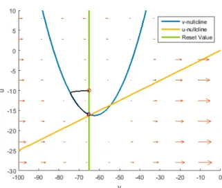
Figure 4.5: This phase plane belongs to the regular spiking neuron. It resets once about 8mV above the initial point, resets again and then it has found a periodic spiking rate, which can also be seen in the next figure.
• CH Neuron
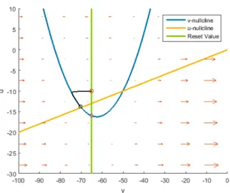
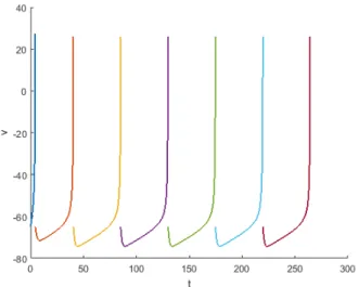
Figure 4.7: This phase plane belongs to the chattering neuron. Here, the bursting behaviour is evident. Since the reset is set at−50mV, the neuron has a lot of time before it is back inside thev-nullcline. That in combination with a low value ford causes these rapid spikes.
4.2 Neuronal behaviour 4 THEORY
• FS Neuron
Figure 4.9: This phase plane belongs to the fast spiking neuron. It is more active than the regular spiking neuron in the sense that itsd value is much lower, removing the part of the orbit that would follow thev-nullcline in case of the RS neuron.
• LTS Neuron
Figure 4.11: This phase plane belongs to the low-threshold spiking neuron. This behaviour resembles the fast spiking neuron, since we are way above the threshold po-tential, the difference is that the fast spiking neuron has a higher vertical field strength, causing a steeper decline.
Figure 4.12: The spike trains that the LTS neuron produces is similar to the RS and the FS neuron, but it differs in the speed of spike train production.
4.3 Microscopic Model 4 THEORY
4.3 MICROSCOPICMODEL
Figure 4.13: The microscopic model in graphic form
Now that the dynamics of the different neurons is known, the simulations of the microscopic model can now be understood. It is important to realize that the microscopic model is more complicated than just a coupled network of 4 types of neurons, it also contains spike-timing dependent plasticity (STDP), a delay in signal transfer and synaptic depression and potency. Spike-timing dependent plasticity influences strength of the synaptic connections. If an in-put spike to a neuron occurs immediately before the outin-put spike of that particular neuron, then that input signal is stronger. The opposite of this process, where the input signal is just after the output action potential, the input signal is made weaker. This is spike-timing dependent plasticity. The process continues until some of the initial connections remain, whereas the influence of all others has become negligible. The other effects, synaptic de-pression and its counterpart, synaptic potency, are long term effects that also have influence on the strength of the synaptic connections. This process works with neurotransmitters that balance the neuronal activity. If neurons would only receive positive feedback, they would eventually reach a state of inactivity or too much activity; this is countered by teamwork of synaptic potency and depression. The networks consists of the four types of neurons de-scribed above.
• Default Simulation - 24 hours with 100 neurons
Figure 4.14: This is a 24 hour (86400 seconds) simulation of 100 neurons. The left figure shows the entire simulation, the right figure is a subset of the left.
4.3 Microscopic Model 4 THEORY
• Default Simulation - 24 hours with 200 neurons
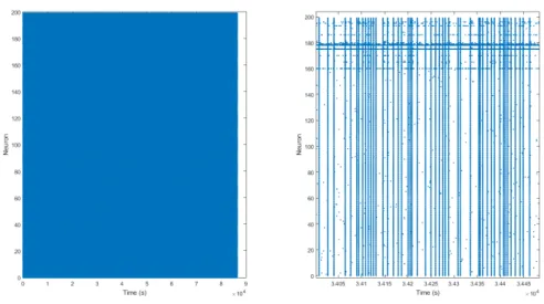
Figure 4.16: This is a 24 hour simulation of 200 neurons. On the left side, the simulation over the full 86400 seconds. The right figure shows a subset of the left.
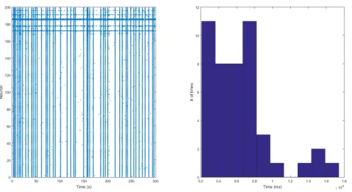
• Default Simulation - 300 seconds
Figure 4.18: The left figure is the model with all its default parameters. Although the right figure does not show an exponential distribution, this is classified as statistically insignificant because the simulation time is short.
4.3 Microscopic Model 4 THEORY
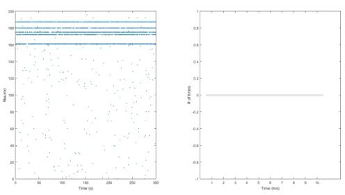
• No Synaptic Connection
Figure 4.20: In the left figure it can be seen that, as expected in the situation of no synaptic connection, there are no population bursts, since the network now consists of 200 individual neurons. The right figure, the histogram, confirms this.
• No Long-Term Effects
Figure 4.22: No long term effects do not cause a significant difference compared to the default simulation. This is expected since the simulation is only 300 seconds long and the long term effects take hours to become active.
4.3 Microscopic Model 4 THEORY
• No Synaptic Depression
Figure 4.24: No synaptic depression shows interesting behaviour. In the left figure, the excita-tory population shows a non bursting regime twice (the two dense pillars), where the activity is much higher. The right figure is a subset of the left.
• Only Chattering Neurons
Figure 4.26: The left figure shows a population with only chattering neurons. This is a good basis for further comparison with the reduced model later. The right figures shows the exponential distribution again.
4.3 Microscopic Model 4 THEORY
• Only Chattering Neurons without Synaptic Depression
Figure 4.28: The figure on the left shows that the population is much more active than with synaptic depression. The right figure does however, show that there is no strange behaviour among bursts.
Both 24 hour simulations were done using the default values of the C++ program [2]. Fig-ures 4.14 up to and including figure 4.17 show the exponential distribution of the inter burst times and the normal appearance of a burst. The short default simulation shows a similar pattern as the long simulations. However, the inter burst times are quite odd in this particu-lar case, but that is due to the length of the simulation. In the long run, these oddities fade under the statistical dominance of the exponential distribution. Hence, the right figure in figure 4.18 is considered statistically insignificant for the conclusion on the type of distribu-tion. In the case of no synaptic connection, which is achieved by setting all parameters that determine the synaptic connection to zero (a=0), it is expected that there are no popula-tion bursts. That is because the input of any neuron does not reach any other neuron. As a result, the neurons in this simulation will only fire upon exceeding their thresholds. No long term effects, achieved by settingam andapto zero, do not have much influence either, but that is also because the simulation times are short. Upon removing the synaptic depression, am=0, the simulation shows very different behaviour. The excitatory population shows the activity pattern in a non-epileptic case (without bursts and quiescence), but the inhibitory population is bursting with a very small inter burst time. Upon adapting the code such that the program simulates only chattering neurons, it is found that the bursts are still finite, but they are longer than normal. This is because the inhibitory population that normally would deactivate the excitatory population has been completely removed. The bursts are still finite due to the way the chattering neurons are modeled. In the phase plane in figure 4.7, the orbit shows a number of quick action potentials, but with an increasingu variable. That means that theu-nullcline is further away for each consecutive spike. As a result, before crossing the nullcline, the orbit descends and after crossing, ascends. That means that the reset after the last spike will always be inside thev-nullcline again, drawing the burst to a halt. Upon removing the synaptic depression, the population of only chattering neurons becomes a lot more active, but does not show any non-epileptic activity; it only bursts a lot more often. This gives an indication that the synaptic depression has a large influence on the activity of a pop-ulation with both inhibitory and excitatory neurons, but mainly on the inhibitory poppop-ulation. It is even so that the large amount of inhibitory bursts damps out the excitatory bursts, which explains the pattern seen in figure 4.24 and 4.25.
5 M
ETHODS5.1 Qualitative approach 5 METHODS
5.1 QUALITATIVE APPROACH
The desired neuronal behaviour is bursting. Therefore one may also look at what exactly makes a neuron burst and more importantly, what makes a neuron stop bursting. A burst is a number of spikes in close proximity. A spike is the output signal of a spiking neuron when the membrane potential is larger than the threshold. Thus bursting means that the membrane potential shortly after firing a spike is again above the threshold, causing the neuron fire an-other spike. This happens a number of times before the membrane potential is below the threshold and quiescence follows. A model can be made from scratch based on biophysically sensible descriptions of neurons, but also mathematically by investigation of the behaviour and simply imitating that with mathematics. Building up a model by means of the qualitative approach is not within the scope of this work, but it is important to know that there are mul-tiple ways to get to a good model. An example of the qualitative approach on microscopic dynamics is the famous Hodgkin-Huxley model, this is a 4-D model with gating variables, which are modeled as voltage dependent variables and act based on earlier voltages, caus-ing highly nonlinear behaviour. A simplification of this particular model is the Izhikevich model, [5] presents this qualitative approach. By giving the mathematical form of the differ-ent spikes that a spiking neuron produces, the Izhikevich model is able to show all forms of neuronal behaviour and is 2-D, allowing for phase plane analysis, as shown in section theory. Also direct population models have been made. A famous example of this is the Wilson and Cowan model.
5.2 MEAN-FIELDREDUCTION- LIF NEURONS
A mean-field reduction has to be done to reduce the number of dimensions drastically and thereby making computations significantly less cumbersome. There are a number of meth-ods available for these types of reductions, which require a number of assumptions.
5.2.1 POPULATIONDENSITYAPPROACH
There is a method to find macroscopic variables for LIF (leaky integrate and fire) neurons. The assumptions that need to be made:
• The nonstationary temporal evolution of the spiking dynamics can be captured by sim-ple models of neurons.
• The dynamics of afferent neurons is neglected.
• The history of each neuron input/output is uncorrelated.
• Every neuron has the same behaviour averaged over time as averaged over space.
across the simulation time, the number of action potentials in that window can simply be counted. It is important to think about what is behind the activity, whether that is because all neurons have approximately the same membrane potential or half of the neurons is above that level and the other half is below. The population density is left to chance, the Fokker-Planck equation for the population density can be derived [3]. In general, neurons with the same state at a certain time have had a different state beforehand compared to each other. That means that the state of all the of the neurons that where initially the same, may have a completely changed at a certain time further. This randomness is caused by fluctuations in the currents. A key assumption to make this model work is to assume that the afferent input currents are in no way correlated with each other. The resulting Kramers-Moyal expansion of the Chapman-Kolmogorov equation is
∂p(v,t)
∂t =
∞
X
k=1 (−1)k
k!
∂k
∂vk
h
p(v,t) lim dt→0
1 dt〈²
k
〉v
i
.
This equation is based on the moments〈²k〉v. We sum over these moments up to infinity. An important question to ask is whether that is necessary. The first two moments of the equation above are the interesting components, called drift (µ) and diffusion (σ2), respectively.
5.2.2 THEDIFFUSIONAPPROXIMATION
• The sums of the synaptic gating variables can be replaced by a fluctuating term and a DC component.
After doing this particular mean-field reduction, it is found that the original model, consisting of numerous equation per leaky integrate and fire (LIF) neuron have become a small number of population equations. Although a LIF neuron is very different from the Izhikevich neuron, the idea that is behind the theory of reduction has a similar character. The population equa-tions are presumably nonlinear and self-consistent. The equation that we found forp(v,t) requires the moments〈²k〉v. The first two moments of the are calculated by simply evaluat-ing the limit
M(k)= lim d t→0〈²
k
〉v= 〈Jk〉N r(t)
5.2 Mean-Field Reduction - LIF Neurons 5 METHODS
from single neuron dynamics to population dynamics is possible, by expressing the infinites-imal change in the membrane potential of the population as [3]
dVE(t)= 〈J〉NErE(t) dt−VE(t)−VL
τE
dt,
dVI(t)= 〈J〉NIrI(t) dt−
VI(t)−VL
τI
dt,
The〈J〉N r term thus denotes the effect of presynaptic output on postsynaptic neurons. We do not yet have an expression forr, but assuming that we can find one, we continue. Now that we have the population dynamics of both types of neurons, we must still realize that these equations do not model any synaptic behaviour, nor the effect of the excitatory neu-rons on the inhibitory and vice versa. In principle, the mpf-rate could be calculated from an experiment, but we want the mpf-rate to be known beforehand. Namely, determining the rate function after simulation means that we end up with an expression that would render every simulation with the same rate function, identical to the first one. Also, no information on bursting can be contained in the rate function by determining it simply from simulations, because the population had shown a more constant activity, we can find the same mpf-rate as for the population that bursts. To account for these temporal effects, it is necessary to construct a peristimulus time histogram (PSTH). This does not change the way in whichr is calculated, but it does grant more insight in what the underlying population is doing. The PSTH is constructed by calculating the number of spikes in a tiny binki and creating a bar based on the number of spikes in that binki.
AE(t)∆t= 1 NE
ˆ t+∆t
t
X
j∈NE
X
f
δ(t−t(jf)) dt,
AI(t)∆t= 1 NI
ˆ t+∆t
t
X
j∈NI
X
f
δ(t−t(jf)) dt.
Returning to the Kramers-Moyal expansion, the infinite sum is now approximated by the drift and diffusion approximation. The resulting equation describing the population density is called the Fokker-Planck equation, given by
∂p(v,t)
∂t =
1 2τσ
2(t)∂2p(v,t)
∂v2 +
∂ ∂v
h³v−VL−µ(t)
τ
´
p(v,t)i.
If the drift is linear and the diffusion is constant, the equation describes an Ornstein-Uhlenbeck process. By definition, the Ornstein-Uhlenbeck process describes the velocity of a massive Brownian particle (a particle doing a random walk), under the effects of friction. In this case the Ornstein-Uhlenbeck process describes the membrane potential evolution under the ef-fects of depolarization. We introduce the flux of probability, defined by
F(v,t)= −v−VL−µ
τ p(v,t)−
σ2 2τ
∂p(v,t)
However, our input current for an individual neuron is still deterministic and given by the presynaptic current of that neuron and external input, the equation forR Iidescribed in 4.2.1. We can rewrite that equation in terms of population variables, the drift and the diffusion, and we add noise to accommodate for random firing of presynaptic neurons.R Iis now given by
R I(t)=µ(t)+σpτw(t).
Herew(t) is a white noise process. The stationary solution of the continuity equation has to agree to the following boundary conditions:
p(θ,t)=0,
∂p(θ,t)
∂v = −
2rτ
σ2 ,
which say that the probability density at the threshold is zero and that the derivative of prob-ability density with respect to the membrane voltage at the threshold gives the average firing rater of the population, respectively. It does this by self-consistent arguments. This means thatr is expressed asr = f(r). The reset function sets the part of the population that is at the threshold back to the reset potential. This can be added to the continuity equation in the following way:
∂p(v,t)
∂t = −
∂ ∂v
h
F(v,t)+r(t−tr e f)H(v−vr eset)i,
H represents the Heaviside step function, which is defined asH(x)=´−∞x δ(s) ds. The solu-tion to this equasolu-tion, satisfying the boundary condisolu-tions that we set, is:
ps(v)=2rτ
σ exp
³
−v−VL−µ
σ2
´
·
ˆ θ−VL−µ σ
v−VL−µ σ
H³x−Vr eset−VL−µ
σ
´
ex2dx.
Neurons are generally not instantaneous in any kind of behaviour that they show, so the reset does not immediately set the neuron back to its starting value, but it takes some time for this to happen. This is called the refractory period and we denote it bytr e f. That means that there is a fraction of the neurons in the population in the refractory period, denoted byr·tr e f. If we take this into account, we get the following equation, describing the probability of the entire sample space, which is the total population. This must equal 1 by the laws of probability.
ˆ θ
−∞
ps(v) dv+r·tr e f =1.
Using the definition ofpsand solving forr, the population transfer functionφis obtained
r=φ(µ,σ)=htr e f+τ
p
π
ˆ θ−VL−µ σ
v−VL−µ σ
ex2(1+erf(x)) dxi−1.
5.3 Analytic Reduction - Izhikevich Neurons 5 METHODS
because this can be generalized for the excitatory and inhibitory populations. The set of stationary, self-reproducing ratesri withi =E,I can be found by solving the coupled self-consistency equations
ri=φ(µi,σi).
To solve the equations that were derived a moment ago for both populations, the differential equations describing the approximate dynamics of the system must be integrated, which has, as fixed-point solutions, the exact equation that was just found. These differential equations each have their own respective time scaleτi withi =E,I. Writing out the indexi for each equation,
τE drE
dt = −rE+φ(µE,σE),
τI drI
dt = −rI+φ(µI,σI).
These equations show that the population firing rate depends on the input current (first-passage time formulaφ), which in turn depends on the firing rate. Thus ther must be deter-mined self-consistently, which is computationally cumbersome, as it requires realistic synap-tic dynamics and higher order corrections. [8] proposes a simplified approach in solving the self-consistent equations.
This shows the theory of behind the one of the most general mean field reductions. But this reduction is for neurons that are described by a single differential equation. It is therefore not suitable for the Izhikevich neuron, but it is important to understand the background of the mean field theory. The analytic approach that will be done next, will seem very different at first glance, but as it will turn out, also a firing rate is found.
5.3 ANALYTICREDUCTION- IZHIKEVICHNEURONS
the set of two interconnected differential equations reduces to a single individual equation, given by
dv
dt =0.04v 2
+5v+140+Λ.
This differential equation is nonlinear, but by means of separation of variables, we can find an analytic solution.
ˆ
dv
0.04v2+5v+140+Λ=
ˆ
dt,
10
p
4Λ−65arctan
³ 2v+125
5p4Λ−65
´
=t(Λ;v).
This solution can be used to find the time it takes forv|v=cto go tov|v=30with caution, since the arctan function is symmetric, which means that there are two solutionstspi kesatisfying
tspi ke(Λ;c)=t(Λ; 30)−t(Λ;c),
a positive one and a negative one. The restriction necessary to find only the positive solution is 0.04c2+5c+140+Λ>0. This is important because the right hand side of the differen-tial equation describing the reduced system has to be greater than zero in order to diverge towardsv|v=30. Inside a burst, the instantaneous firing rate is now determined as the recip-rocal of the inter spike times, since every spike follows directly after the other. The bursting neuron (CH neuron) is achieved when there is no equilibrium point. To make sure that the equilibrium point is absent, theu-nullcline has to be cut alongv|v=cinto two parts, of which the right part has to be raised. This raise is achieved by introducingfmi n, the minimum firing rate for a neuron at which it can still be called a bursting neuron. This also has a physiological meaning, since large cells have lower firing rates that small ones. The minimum firing rate is given by
fb(Λ;c)=
max³Ts(1Λ;c),fmin
´
0.04c2+5c+140+Λ>0,
fmin otherwise.
Yet, not every neuron is always bursting, distinction must be made between bursting and non-bursting. The actual firing rate becomes
f(v,Λ;c)=Hω(v−c)fb(Λ;c).
Here, Hω is the smooth approximation to the Heaviside step function, with steepness pa-rameterω. This function is centered round the reset to distinguish between bursting and non-bursting. The functionHωis defined as
5.3 Analytic Reduction - Izhikevich Neurons 5 METHODS
The resetv←cis now taken care of, but the reset has an additional termu←u+dwhich is not yet in the reduced model. We can introduce this by adding the firing rate function to the dynamics ofu. Since every spike causesuto be raised withd, the reduced recovery variable urdepends ond f, the time averaged increase rate
dur
dt =a(bvr−ur)+d·f(vr,Λ;c).
5.3.1 CH NEURONS
The branch is still not added to the phase plane. So far, theu variable has been adapted and the firing rate f was determined. The shape and exact position of the branch does not matter, except for its maximum, which must be at the same height as the intersection of the v-nullcline withc. The branch can be added by incorporating an additional term in the system of DEs. The new system of DEs becomes
dvr
dt =0.04v 2
r+5vr+140−ur+I−ξeη(vr−c), dur
dt =a(bvr−ur)+d f(vr,ur,I;c).
There has to be a difference between neuron behaviour and since the chattering neurons are the ones that produce bursts, the new branch is determined for this type first. Letnvdenote thev-nullcline andnvr denote thevr-nullcline, which contains the new branch. n0vr is the derivative of thevr-nullcline with respect to the potential. Then the following equations must hold.
nv(v)=0.04v2+5v+140+I,
nvr(v)=nv(v)−ξe η(v−c),
nvr(c+κ)=nv(c,
n0vr(c+κ)=0.
The horizontal separation is given byκ. Upon solving these equations, we find:
η= n
0
v(c+κ) nv(c+κ)−nv(c),
ξ=nv(c+κ)−nv(c)
eηκ ,
plane of the chattering neuron can now be generated and a comparison can be made with v−tgraph in order to compare the accuracy of the reduction.
Figure 5.1: This phase plane belongs to the reduced chattering neuron. The reset is gone, thus also the spikes, it is now a smooth approximation to the dynamics with the reset.
5.3 Analytic Reduction - Izhikevich Neurons 5 METHODS
5.3.2 RS, FSANDLTS NEURONS
To avoid the reset for the periodically spiking neurons, it is necessary to do a similar reduc-tion. However, the resetcis now on the left-hand side of the minimum of thev-nullcline. That means that the branch cannot simply be added in the same way as before, since the neuron will fire only after going past that minimum. To leave the subthreshold behaviour intact, a slightly different approach is necessary. The additional branch must be shifted to the right further than before. That is because the constraints that have been set require a separation distanceκto hold. Thisκ>5, because
• The intersection of thev-nullcline and the reset valuecis at−65mV and the minimum of thev-nullcline is at−62.5mV, thus the distance between them is 2.5.
• Thev-nullcline is a parabola, thus symmetric around its minimum.
• The distance between the intersection just described and its mirror image is thus 5.
• For the constraints to be valid,κ>5.
Ifκis chosen smaller,ηandξwill become negative and turn the branch 180 degrees around turning pointv−c. That will completely demolish the dynamics. This problem is solved in [7] by setting the reset valuec at−55mV which is to the right of thev-nullcline, thus any
κ∈[0.5, 2.5] suffices. The constraints as they were set in the paragraph on chattering neurons can be left intact in both cases. The coupled population model that is presented in at the end of the paragraph Results will usec= −55mV for the neurons that are not the chattering neurons as well, since theκapproach requires a significant amount of numerical computing and testing.
Figure 5.3: The firing rate for the unreduced single cell dynamics of the RS neuron.
By adapting theκvalue such that the reduction shows the samef−I diagram, a good value is found. This is not done here because of the time it takes to find such a good value. Also, for the inhibitory neurons, this approach is slightly different, because theu-nullcline is in at an other position. This altogether makes up for a very time expensive process.
5.3.3 COUPLING
The single cell dynamics with a reset function have now been transformed into reduced sin-gle cell dynamics. Populations dynamics are desired, thus the global activity is taken into consideration. A network ofN neurons can be randomly connected by letting the output of a neuron by the synaptic input of the post-synaptic neuron. It is assumed that the out-put, a spike, produces a spike in the synapse as well. The response of the synapse isq(t−tˆ), such that the linear operatorQ makesQ q=δ, which is the response that is desired. In [7] Q=ddt +α. The spike ˆt is simply the time at which a spike arrives at the synapse. The post-synaptic current becomes
Ipost=g q(t−tˆ)(vpost−vr ev).
Here,gis the maximal conductance,Vr evis the associated reversal potential andVpost is the membrane potential of the post-synaptic neuron. For any neuronia duration
Ti(t)={ˆtj,j∈N| 0<tˆ1<...<tnˆ ≤t}
collects all (or none, the set may be empty) spikes of the neuron in that duration. Define the synaptic activationsi of the post-synaptic neuron as the convolution sum of the spike times Ti with the response of the synapseq(t−tˆ). Thus
si(t)= X
ˆ t∈Ti(t)
5.3 Analytic Reduction - Izhikevich Neurons 5 METHODS
SinceQ q=δ, this is equivalent to
Q si(t)= X
ˆ t∈Ti(t)
δ(t−tˆ).
Not all neurons are connected to each other and they are also not connected with uniform synaptic weight. LetJi j represent the synaptic efficacy as before. ThenJi j=0 means that neuroni is not connected to neuron j and Ji j =1 means that the post-synaptic signal of neuron j is felt byi in the same amplitude that the signal when it left neuron j. The post-synaptic current departing from neuronjtowards neuroniis given by
Is yn,i(t)=g N
X
j=1
Ji jsj(t)(vi(t)−vr ev).
Now that the individual neurons can be coupled by means ofIs yn,i, there is still nothing said about population dynamics. By means of three assumptions, it is possible to find lumped network activity.
• The exact time that a spike arrives at a post-synaptic neuron is not necessary. The in-dividual spike trains can be averaged by representing them with the firing rate. This comes down to replacing the single cell dynamics of an Izhikevich neuron by the re-duced system. The post-synaptic signal is then described by
Q si=f(vi,ui,Iext−Is yn,i).
Iext is the average external input to the neurons.
• The neurons are connected randomly, but there is a lot of knowledge about how many connection a single neuron has in specific regions of the brain. LetW be the random variable describing the synaptic weights, such that the synaptic weights Ji j are dis-tributed independently in the same way thatW is. Define
〈Ji j〉 =EW,
S(t)=
N
X
i=1 si(t).
• Now the most important assumption. Neurons that receive a similar input react also similarly, so they remain close to each other in phase space. It is therefore sufficient use the following averages to approximate the membrane potential and the recovery variable.
v(t)= 1
N N
X
This makes the dynamics of the population dv dt = 1 N N X
i=1
0.04vi2+5vi+140−ui+Iext−Is yn,i−ξeη(vi−c) ≈g(v,u,Iext−Is yn),
du dt = 1 N N X
i=1
a(bvi−ui)+d f(vi,ui,Iext−Is yn,i;c) ≈h(v,u,Iext−Is yn),
g(v,u,Iext−Is yn)=0.04v2+5v+140−u+Iext−Is yn−ξeη(v−c), h(v,u,Iext−Is yn)=a(bv−u)+d f(v,u,Iext−Is yn;c).
Is yn(t)=g〈Ji j〉S(t)(v(t)−vr ev).
The post-synaptic signal depends on the firing rate and on the number of neurons. The final equation for the reduced model becomes
QS=N f(v,u,Iext−Is yn).
6 RESULTS
The dynamics of the population are now described by three differential equations. The exter-nal currentIextis a noise term, thus the DE describingvis stochastic in nature. This means that using MATLAB’s standard ODE solvers are not useful, because they solve only determin-istic systems of equations. Although MATLAB itself does have some stochastic differential equation solvers, a simple adapted Euler forward approach will suffice here. Therefore, the reduced model is constructed using the Euler-Maruyama scheme. In its formal definition, the Euler-Maruyama scheme is as follows. Consider a stochastic differential equation in a general form
dX=f(X) dt+g(X) dW,
whereW is a Wiener process. Upon solving this SDE on some time interval [0,T], the Euler-Maruyama approximation to the true solutionX is a Markov chainY. By making a partition of the interval [0,T] in pieces of dt>0, with dt=T/N, withN the number of subintervals, the SDE can be rewritten into
Y[n+1]=Y[n]+f(Y[n]) dt+g(Y[n]) dW,
dW =W[n+1]−W[n].
The latter expression can be rewritten into a simpler term, sinceW is a collection of simply a normal distributed random variables that describe a white noise process. The SDE for the membrane potential does not contain such a functiong(X), the noise term is simple. The final formal definition of the Euler-Maruyama scheme becomes:
6 RESULTS
Here,Bis a random number drawn from a normal distributionN(0, 1) andσis the variance of the noise. Now the equations that were found in the previous paragraph can be discretized. The system in this scheme looks as follows:
v[n+1]=v[n]+
³
0.04v[n]2+5v[n]+140−u[n]−ξexpη(v−c)−Is yn´dt+σpdt B,
u[n+1]=u[n]+³a(bv[n]−u[n])+d f(v[n],u[n],Iext−Is yn;c´dt,
S[n+1]=S[n]+³−αS[n]+N f(v[n],u[n],Iext−Is yn;c)´dt,
withn=0, 1, 2, ...
The square brackets here denote that the functionsv,uandSare now discrete. This can as it is, be inserted into MATLAB with the right values for the constants and deliver a nice model for a single population of identical neurons. For a small simulation (30 seconds), the algo-rithm is fast and reasonably reliable. It is not great as it may in some cases explode. By doing longer simulations, the inter burst period may be analyzed to verify the quality of the reduc-tion. If all is well, the inter burst period is exponentially distributed.
6 RESULTS
Figure 6.2: A 300s simulation. The top left figure shows the average membrane potential. The top right figure shows the phase plane, which has exactly the same shape as the reduced single cell phase plane. The inter burst times are approximately expo-nentially distributed as shown in the bottom left figure. The bottom right figure shows a subset of the top left.
have on each other, thus determining the average synaptic weight. This can be modeled by using the scheme above and adapt it for the number of populations. First, it is verified that the dynamics are the same as in the previous simulations. By means of a short simulation (30s) and looking at the phase plane of the populations, it can be seen that the dynamics are fine.
Figure 6.3: The left figure shows the phase plane with the two excitatory subpopulations and one inhibitory. Since they have the same shape as in figure 6.1 and 6.2, the dy-namics are correct. The right figure shows the average membrane potential of the three individual subpopulations.
TheIs yn variable contains the information of the surrounding populations. These coupling equations have been copied from [7].
Is yni nh=Gi nhexc2·Sexc2[n−1]
³
Eexc−vi nh[n−1]
´
Is ynexc1=Gexci nh1·Si nh[n−1]³Ei nh−vexc1[n−1]
´
Is ynexc2=
³
Gexcexc12·Sexc1[n−1]+Gexcexc22
´³
Eexc−vexc2[n−1]
´
Here,Gij determines the conductance from population j to populationi and is depending on the number of cells in networkj. Its definition is
Gi nhexc1=Ni nh·pi nhexc1·gexci nh Gexcexc12=Nexc1·pexcexc12·gexcexc21 Gexcexc22=Nexc2·pexcexc22·g
exc2 exc2 Gi nhexc2=Nexc2·pi nhexc2·gi nhexc2
6 RESULTS
Excitatory 1 Excitatory 2 Inhibitory
Parameter Value Parameter Value Parameter Value
a 0.01 a 0.03 a 0.02
b 0.2 b 0.3 b 0.2
c -50 c -55 c -55
d 2 d 2 d 2
Iext 3 Iext 3 Iext 2
Eexc 0 Ei nh 0
The connectivity parameters are set at:
Parameter Value Parameter Value pi nhexc1 0.3 gexci nh1 0.02 pexcexc21 0.1 gexcexc21 0.02 pexcexc22 0.1 gexcexc22 0.005 pexci nh2 0.1 gi nhexc2 0.02
A simulation with this setup containing 100 inhibitory neurons and 600 excitatory neurons (300 of each sort) withσ=1 gives
Figure 6.4: From the phase plane in the left figure it can be seen that there is something wrong in the coupling. The right figure shows the three individual populations, from which it can be seen that the exc2-population is malfunctioning.
Figure 6.5: From the phase plane in the left figure it can be seen that the populations are inactive. The right figure shows that three individual populations are all at rest.
This last simulation in figure 6.5 shows no spikes or bursts, the populations are at rest. That indicates once more that the coupling is incorrect, since it does not give the same results as in [7]. Upon redefining the coupling correctly, the simulations of coupled populations must turn out fine as well.
7 D
ISCUSSION8 CONCLUSIONS
coupled population level, which is unfortunate. On single population level, the simulations of the macroscopic model are in accordance with the microscopic model.
Experiments may be done to verify the macroscopic model. Apart from verification, it would also be interesting to see the influence of synaptic depression on the inhibitory population and the excitatory population. From the numerical simulations of a coupled population and an isolated excitatory population, it appeared that the synaptic depression had a significant influence on only the inhibitory population, as a short term effect. If the synaptic depression causes so much activation in the inhibitory population, the excitatory population will not burst.
8 CONCLUSIONS
9 REFERENCES
[1] T.A. Frewen C.R. Laing and I.G. Kevrekidis. Reduced models for binocular rivalry.Journal of Computational Neuroscience, 28:459–476, 2010.
[2] J. Dijkstra. Adaptation to low frequent stimuli in computational and cultured neuronal networks.University of Twente, 2014.
[3] P.A. Robinson M.Breakspear G. Deco, V.K. Jirsa and K. Friston. The dynamic brain: From spiking neurons to neural masses and cortical fields. PLoS Computational Biology, 4, 2008.
[4] E.M. Izhikevich. Simple model of spiking neurons.IEEE Transactions on Neural Networks, 14, 2003.
[5] E.M. Izhikevich. Which model to use for cortical spiking neurons. IEEE Transactions on Neural Networks, 15:1063–1070, 2004.
[6] H. Markram M. Tsodyks, K. Pawelzik. Neural networks with dynamic synapses. Neural Computation, 10:821–835, 1998.
[7] S. Visser and S.A. Van Gils. Lumping izhikevich neurons. EPJ Nonlinear Biomedical Physics, 6, 2014.
10 APPENDICES
10 APPENDICES
10.1 APPENDIXAThe C++ program [2] is executed on a windows 8 platform. The compiler used is of a g++ nature, Netbeans 8 namely. This compiler will not work on windows without an UNIX envi-ronment and a backup program. These are Cygwin and MinGW respectively. Apart from the standard Netbeans libraries, also the boost library will need to be downloaded. When this is all set up correctly, the program may be run. The values that were used in the 24 hour simu-lations are the default values. It is important to realize that this program is computationally expensive in the sense that simulations with more than 250 neurons take longer in real time than its eigentime. This means that if one wishes to simulate 300 neurons over 500 seconds (called the eigentime), the real time simulation may take over 1000 seconds.
10.2 APPENDIXB