Parametric inference for functional information mapping
Dennis Leech, Robert Leech and Anna Simmonds
No 899
WARWICK ECONOMIC RESEARCH PAPERS
Parametric inference for functional information mapping
Robert Leech
Division of Neuroscience and Mental Health Imperial College London
Anna Simmonds
MRC Clinical Sciences Center, Imperial College London
Dennis Leech Department of Economics
University of Warwick
1
abstract
An increasing trend in functional MRI experiments involves discriminating between ex-perimental conditions on the basis of fine-grained spatial patterns extending across many voxels. Typically, these approaches have used randomized resampling to derive inferences. Here, we introduce an analytical method for drawing inferences from multivoxel patterns. This approach extends the general linear model to the multivoxel case resulting in a vari-ant of the Mahalanobis distance statistic which can be evaluated on the χ2 distribution.
We apply this parametric inference to a single-subject fMRI dataset and consider how the approach is both computationally more efficient and more sensitive than resampling inference.
2
Introduction
In tandem with the search for activation differences - and gaining momentum in recent years - are approaches that search for information across multiple voxels. Analyzing for information involves assessing whether there is sufficient information to distinguish be-tween two conditions across all the voxels in a given region (Haxby et al. 2001) or even across all the voxels in the brain (Hanson and Halchenko 2008), irrespective of the level of activation of a given voxel. By taking advantage of the fine spatial patterns across voxels, information-based approaches have become highly adept at detecting subtle differences in signal between conditions (Kay et al. 2008, Mitchell et al. 2008).
Kriegeskorte and colleagues (Kriegeskorte et al. 2006, Kriegeskorte and Bandettini 2007) proposed an information-based approach that attempts to reconcile the sensitiv-ity of multivoxel analyses with the spatial localization of activation-based analyses. With this approach, a spherical searchlight was passed around the brain centered on each voxel, and a multivoxel distance statistic was calculated across all voxels within the searchlight. The Mahalanobis distance statistic was shown to be substantially more sensitive at detect-ing signals than standard univariate t-statistics or Euclidean distance measures. Variants of this statistic have been used successfully in several fMRI experiments within the visual domain (Kriegeskorte et al. 2006; 2007, Serences and Boynton 2007a;b, Stokes et al. 2009). The Mahalanobis distance (Mahalanobis 1936) is a multivoxel similarity measurement that unlike Euclidean distance is scale invariant and controls for covariance across the dat-apoints. In fMRI datasets, the Mahalanobis distance can calculate the similarity between different experiment conditions, e.g., how dissimilar are visual and auditory processing for a given set of voxels. This statistic controls for error covariance across voxels; spatially correlated error is expected in fMRI datasets given spatial patterns of sources of noise affecting the BOLD signal, such as vasculature, movement artifacts etc. To calculate the Mahalanobis distance, Kriegeskorte et al. (2006) fitted a separate GLM analysis to the unsmoothed functional data for each voxel. The Mahalanobis distance was then calculated using the resulting vectors of beta weights and the residual error covariance matrix across voxels
∆ =(βˆ2−βˆ1)!Σ−1(βˆ2−βˆ1) (1)
whereβˆ1 and βˆ2 are vectors of estimated regression coefficients associated with two types of stimuli andΣˆ is the error covariance matrix.
test). Most importantly, for typical fMRI datasets, parametric techniques can be several orders of magnitude more computationally efficient than resampling methods. As such parametric inference for across-voxel Mahalanobis distance would be a useful tool for ana-lyzing for information rather than activation differences in fMRI data.
In this paper we demonstrate how parametric inferences can be drawn based on the Mahalanobis distance. We set out how the Mahalanobis distance relates to the general linear model and how it can be evaluated analytically on the χ2 distribution. We then
apply the parametric Mahalanobis analysis to an example fMRI data. Finally, we compare parametric inference based on the Mahalanobis statistics with inference derived using re-sampling.
3
Theory
3.1 The statistical model
We start with the GLM as applied to fMRI datasets (Friston et al. 1994). We assume the response by each voxel can be modelled by a regression model written as follows.
yit= k
!
h=1
βhixht+uit (2)
where i is the voxel subscript, i = 1, ..., n, and t is the time subscript, t = 1, ..., T. βhi
represents the response of voxel ito the stimulus measured by regressorh.
This can be written using matrix algebra as,
yi =Xβi+ui (3)
whereyi is theT element observation vector for voxeli,X theTxkinput matrix,ui theT
element error vector, andβi thekelement coefficient vector. There is a different regression
model for each voxel but all models have a common regressor matrix.
The error for each voxel equation is assumed to have zero mean, be serially independent and homoscedastic, but correlated across equations.
That is, E(ui) =0 for alli andE(uiu!j) =σijIT for all iand j.
This can be written more compactly as:
where y= y1 y2 ... yn ,u=
u1 u2 ... un ,β=
β1 β2 ... βn ,Z=
X 0 . . . 0
0 X . . . 0
... ... ... ... 0 0 . . . X
=In⊗X,
Ω=
σ11IT σ12IT . . . σ1nIT σ12IT σ22IT . . . σ2nIT
... ... ... ...
σ1nIT σ2nIT . . . σnnIT
=Σ⊗IT,and Σ=
σ11 σ12 · · · σ1n σ12 σ22 · · · σ2n
... ... ... ...
σ1n σ2n · · · σnn
.
It is well known (Zellner 1962) that, when there is a common set of regressors, the correlation of the errors in different equations can be ignored in coefficient estimation and least squares applied separately to each equation. That is, the efficient estimator of the complete system is:
ˆ
β=(Z!Z)−1Z!y,and therefore βˆi =(X!X)−1X!yi. (5)
The covariance matrix ofβˆis
V(βˆ) = (Z!Z)−1Z!ΩZ(Z!Z)−1. (6)
Noting that
Z!Z= [In⊗X!][In⊗X] =In⊗X!X, and hence that (Z!Z)−1=In⊗(X!X)−1,
and that
Z!ΩZ= [In⊗X!][Σ⊗IT][In⊗X] =Σ⊗(X!X),
we can rewrite (6) as
V(βˆ) = [In⊗(X!X)−1][Σ⊗(X!X)][In⊗(X!X)−1] =Σ⊗W, (7)
where (X!X)−1 =W. From this we obtain the covariance between any pair of estimated
coefficients as
Cov( ˆβgi,βˆhj) =σijwgh (8)
3.2 Inference
We are interested in testing a set of linear restrictions on coefficients across the separate equations for each voxel. In general there areghomogeneous restrictions written asRβ = 0
whereRis ag×nkmatrix of given constants of rankg. In the next two subsections we use
this framework to derive tests for the following restrictions: (1) that a coefficient of a par-ticular stimulus is equal to zero in all voxels, and (2) that two effects are equal in all voxels.
If the equation errors uit are gaussian then the efficient estimator of β given in
equa-tion (5) is normally distributed and the well known (see for example Rao and Rao 1973) inferential procedures for generalised linear regression models are available based on the covariance matrix in equation (6), (7) or (8). This only holds exactly ifΣ is known and does not have to be estimated. The alternative approach, a Wald test adopted here, is to use large sample procedures based on the asymptotic normality of βˆ (which does not
depend on any particular assumption about the form of the distribution of the random errors) and the use of a consistent estimator ofΣ. (See for example Greene (2003).)
The null hypothesis of interest is written as
H0:Rβ = 0. (9)
Letting Rβ = δ this can be written as H0 : δ = 0. Now let Rβˆ = ˆδ. Then δˆ is
asymptotically normally distributed with expectation E(ˆδ) = 0 and covariance matrix V(δ) =ˆ RV( ˆβ)R!. We call the test statistic ∆, given by
∆ =ˆδ![RV( ˆβ)R!]−1δˆ (10)
which has an asymptotic χ2 distribution with g degrees of freedom ifH
0 is true.
Testing a single coefficient value
Let us consider testing the null hypothesis that one particular coefficient is zero in all voxel equations. We assume that the coefficient is indexed number 1 in each voxel equation.
The null hypothesis is:
H0 :β1i= 0 fori= 1, ..., n, (11)
which can be written in vector notation as
where
β1=
β11 β12
...
β1n
.
These coefficients can also be written as linear functions of the complete coefficient vector as,
β1= [In⊗e!1]β
wheree!1 is a k-element vector whose first element is 1 and all others zeros: the first row
ofIk. Here we can write R=In⊗e!1,δ=β1.
We can thus obtain the covariance matrix of βˆ1 from that of βˆ and use it with the standard theory of testing linear restrictions. We know that
V( ˆβ1) = [In⊗e!1]V(βˆ)[In⊗e1] = [In⊗e!1][Σ⊗W][In⊗e1](from (7))
=Σ⊗e!1W e1 =w11Σ. (12)
This assumes that the elements of Σare known. They can be estimated consistently from the residuals, using,
ˆ
σij = (yi−Xβˆi)!(yj−Xβˆj)/T (13)
We can therefore test the null hypothesis using the likelihood ratio statistic,
∆1=βˆ1
!ˆ
Σ−1βˆ1/w
11 (14)
which, for large T, is distributed asχ2 with n degrees of freedom on H
0. We could also
have obtained the covariance matrix ofβˆ1 directly from expression (8).
Testing coefficient equality
and x2, we test a set of linear restrictions in the null hypothesis
H0:β1i =β2i fori= 1,2, ..., n. (15)
We can write these restrictions, in vector notation, as:
H0 :β1−β2 =0
whereβ2 = [In⊗e2!]β ande2 is defined, analogously to e1, as a vector of all zeros except
for element 2 which equals 1.
Letting δi=β1i−β2i for eachi andδ=β1−β2 =
β11−β21 β12−β22
...
β1n−β2n
, we can write
δ= [In⊗(e1−e2)!]β.
In this case we have R=In⊗(e1−e2)!.
Therefore the covariance matrix ofδˆis
V(δˆ) = [In⊗(e1−e2)!][Σ⊗W][In⊗(e1−e2)]
=Σ⊗(e1−e2)!W(e1−e2) = (w11+w22−2w12)Σ (16)
The test statistic is then
∆2=ˆδΣˆ−1δˆ/(w11+w22−2w12) (17)
with asymptotic null distributionχ2 with ndegrees of freedom.
The statistic in equation (17) is the Mahalanobis distance measure between the vectors
ˆ
β1−βˆ2 (Mahalanobis 1936).
Computation by data transformation and reparameterisation
∆2 in equation (17) can be computed easily using a simple data transformation before
fit-ting the regression and then using ∆1 to test one coefficient in the transformed regression.
Rewriting equation (2) for voxel i,
yit= k
!
h=1
as
yit =β1ix1t+β2ix2t+. . . ,
to highlight the two coefficients of interest, then adding and subtracting the same term on the RHS enables us to derive a new equation with a transformed coefficient and a transformed variable. Thus,
yit=β1ix1t+β2ix2t−β2ix1t+β2ix1t+. . .= (β1i−β2i)x1t+β2i(x1t+x2t) +. . .
Therefore the regression equation can be written:
yit=δix1t+β2ist+. . . .
and the coefficient onx1i becomesδi defined above as a result of the simple data
transfor-mation of replacingx2tby a new variable st defined as the sum of x1t andx2t.
This is computationally very simple but does require running two regressions if we wish to test both sets of restrictions (11) and (15).
4
Example: single subject fMRI data
We applied this method to fMRI data acquired from a single subject. This allowed com-parisons of the Mahalanobis distance statistic (i.e., 17) using different inference methods (both the analytic method described and using resampling).
4.1 fMRI experiment
The fMRI data was acquired from a pilot subject in an experiment investigating bilingual speech production. The subject was a 32-year old neurologically healthy, right-handed male and gave informed consent according to local ethics procedures. The subject viewed color and black and white pictures and was asked to describe the pictures in either his native (English) language or proficient non-native (Spanish) language. A third condition involved a picture prompting the subject to silently move his tongue. The rest baseline involved observing a color picture while remaining silent and still.
The fMRI data was acquired with a Philips Intera 3.0 Tesla scanner using dual gradients and a phased array head coil. Images were obtained using a T2*-weighted, gradient-echo, echoplanar imaging (EPI) sequence with whole-brain coverage (TE, 30 ms; flip angle, 90◦).
Thirty-two axial slices were acquired with a slice thickness of 3.25 mm and an interslice gap of 0.75 mm (resolution 2.19 × 2.19 × 4.0 mm; field of view, 280 × 224 ×128 mm).
software (Psychology Software Tools) was used to present stimuli using the IFIS-SA sys-tem (In Vivo Corporation).
A sparse fMRI design was used to minimize movement- and respiratory-related artifact commonly associated with speech production. Each TR lasted 10 seconds including 2 sec-onds of image acquisition followed by a seven secsec-onds of speech production and one second of rest. The subject was scanned twice with 72 TRs in each 12 minute run.
4.2 fMRI analysis
All images were registered to the middle functional image of the first run using 3dvolreg (AFNI toolbox, Cox et al. 1996). A single time series was created by concatenating the images from the first and second runs. No other preprocessing was carried out.
We restricted all our analysis to a broad anatomically defined region of interest, to re-duce the computational requirements of resampling methods used to validate the paramet-ric evaluation of the Mahalanobis distance. The region of interest was defined in MNI152 space using the probabilistic Harvard-Oxford anatomical atlas from fslview. The region of interest contained the inferior frontal gyrus (pars opercularis and pars triangularis); these regions have been reported in previous studies comparing speech production in different languages (e.g., Hernandez et al. 2001). To allow a spread of voxel activation patterns, the region of interest also included the superior frontal gyrus, less likely to be involved in bilingualism based on previous imaging studies. The region of interest was warped into the subject’s functional space and registered to the subject’s functional scans using FLIRT (Jenkinson and Smith 2001).
A general linear model was fitted to the unsmoothed time series for each voxel in matlab (Mathworks, 2007b). The GLM estimated nine parameters for each voxel: three parame-ters of interest (speaking in native language, non-native language and tongue movement), as well as three parameters for each run to account for mean, linear and quadratic trends. To account for the hemodynamic delay, the labels for each image (i.e., native language, non-native language, tongue movement and rest) were temporally shifted one timepoint (this is equivalent to convolving the dataset with the canonical hemodynamic function in AFNI).
4.2.1 Multivoxel parametric inference
Maha-lanobis distance between native and non-native speech production was calculated using equation (17) which was evaluated with reference to the χ2 distribution. The resulting
p-value were then assigned to the center voxel.
4.2.2 Multivoxel nonparametric inference
We also assessed significance of the statistic in equation (17) using nonparametric random-ized resampling methods. A null-distribution of test-statistics was calculated for each voxel by shuffling the labels (native, non-native, tongue) of each non-baseline block a 1000 times. Each of these 1000 randomized time courses was then analyzed as above. The distribution of randomized test statistics was then sorted and the rank order (divided by 1000) of the unpermuted test statistic provided a p-value.
4.2.3 Univoxel parametric inference
We also aimed to replicate the findings of (Kriegeskorte et al. 2006) regarding the power of the information-based approach over more traditional activation-based analyses. To this end, we reran the GLM for each voxel, but following spatial averaging across all voxels within the spherical searchlight (to increase signal to noise). We subsequently calculated t-statistics at each voxel for the contrast comparing native language with non-native lan-guage.
4.3 Results
4.3.1 Validating the parametric measure
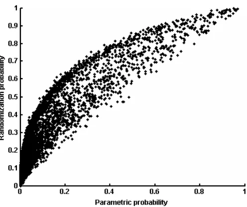
To validate that the multivoxel parametric inference is comparable to the resampling ap-proach proposed by (Kriegeskorte et al. 2006), we compared the p-values derived from equation (17) with p-values derived from resampling (following the method employed Kriegeskorte et al). Figure 1 compares the two inference methods at each voxel across the region of interest, indicating a strong correlation between the resulting p-values from the two methods (Pearson’s r=0.90, Spearman’s rho = 0.96). Figure 1 also indicates that the parametric inference method produces more significant p-values than the randomiza-tion method for every voxel in the region of interest. Thus, the two inference measures appear to agree on the spatial characteristics of the underlying signal, but the parametric approach appears to be more sensitive.
Figure 1: Scatter plot of parametric- and randomization-derived p-values for each voxel in the region of interest.
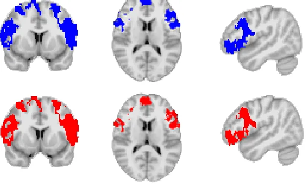
multiple comparisons). This map is nearly identical to the parametric-derived map that is thresholded at the far more stringent p<0.003.
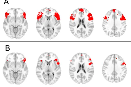
4.3.2 Multivoxel parametric inference and univoxel t-statistic
Figure 3 demonstrates the substantial increase in signal detection for the multivoxel para-metric inference over the more traditional univoxel t-stastics map. Figure 1A and FIgure 1B both display voxels thresholded at the same p-value - determined by applying false discovery rate (FDR, q<0.05 Genovese et al. 2002) to the p-value map derived from the
Figure 2: Comparison of parametric (in blue) and randomization (in red) derived p-values. The parametric map is thesholded at p<0.003; the randomization map is thresholded at
p<0.05. The statistical maps have been projected onto the MNI152 2mm×2mm ×2mm
Figure 3: A: superthreshold voxels determined using multivoxel parametric inference cal-culated across 2 voxel radius spherical searchlights, on unsmoothed data, thresholded at p<0.0086; B: Superthreshold voxels associated with smoothed data and a univoxel t-test,
5
Discussion
In this paper, we have demonstrated how multivoxel information-based inference can be accomplished parametrically by extending the general linear model. We have shown how an instantiation of the multivoxel Mahalanobis distance statistic proposed for fMRI by Kriegeskorte et al. (2006) can be evaluated with theχ2 distribution. Parametric inference
is a more powerful and more computationally efficient alternative to the resampling infer-ence methods used previously. This is a potentially highly efficient and powerful approach to detect differences in blood oxygenation levels with high spatial frequency of the kind that are likely to occur in many cognitive and perceptual tasks.
The proposed approach has two principal benefits over randomization resampling infer-ence methods used for multivariate statistics: 1) efficiency; and 2) sensitivity. Efficiency: the parametric inference involves fitting one model to each voxel, rather than fitting>1000
models to generate a null distribution. As such, this method is at least three orders of mag-nitude more computationally efficient than randomization inference, making information analyses more feasible for many fMRI experiments, including analyses involving the whole brain. Sensitivity: as with parametric approaches in general when distributional assump-tions are met, we find that the parametric inference method detects significant voxels at a much lower thresholds when compared to randomization-based inference. Furthermore, with the example fMRI dataset analysed here we confirm previous studies, suggesting that the Mahalanobis distance method has considerably greater sensitivity to detect a signal than univoxel analyses following spatial smoothing.
The proposed multivoxel parametric inference can also be adapted for group fMRI anal-yses. The Mahalanobis distance can be calculated for each subject and then the statistical maps can be warped into standard space and compared across subjects. Since independent
χ2 statistics are additive, the statistical maps ofχ2 values can be combined across subjects
to create a group statistic that can be evaluated on the χ2 distribution with the summed
degrees of freedom. This is a parametric version of the randomization approach taken by (Kriegeskorte et al. 2007).
References
Cox, R. et al. (1996). AFNI: software for analysis and visualization of functional magnetic resonance neuroimages. Computers and Biomedical Research, 29(3):162–173.
Friston, K., Holmes, A., Worsley, K., Poline, J., Frith, C., Frackowiak, R., et al. (1994). Statistical parametric maps in functional imaging: a general linear approach. Human
Brain Mapping, 2(4):189–210.
Genovese, C., Lazar, N., and Nichols, T. (2002). Thresholding of statistical maps in functional neuroimaging using the false discovery rate. Neuroimage, 15(4):870–878.
Greene, W. (2003). Econometric analysis. Prentice Hall Upper Saddle River, NJ.
Hanson, S. and Halchenko, Y. (2008). Brain reading using full brain suport vector machines for object recognition: There is no ”face” identification area. Neural Computation, 20:486–503.
Haxby, J., Gobbini, M., Furey, M., Ishai, A., Schouten, J., and Pietrini, P. (2001). Dis-tributed and overlapping representations of faces and objects in ventral temporal cortex.
Science, 293(5539):2425–2430.
Hernandez, A., Dapretto, M., Mazziotta, J., and Bookheimer, S. (2001). Language switch-ing and language representation in Spanish-English bilswitch-inguals: an fMRI study.
Neu-roImage, 14:510–520.
Jenkinson, M. and Smith, S. (2001). A global optimisation method for robust affine regis-tration of brain images. Medical Image Analysis, 5(2):143–156.
Kay, K., Naselaris, T., Prenger, R., and Gallant, J. (2008). Identifying natural images from human brain activity. Nature, 452(7185):352–355.
Kriegeskorte, N. and Bandettini, P. (2007). Analyzing for information, not activation, to exploit high-resolution fMRI. Neuroimage, 38(4):649–662.
Kriegeskorte, N., Formisano, E., Sorger, B., and Goebel, R. (2007). Individual faces elicit distinct response patterns in human anterior temporal cortex.Proceedings of the National
Academy of Sciences, 104(51):20600.
Kriegeskorte, N., Goebel, R., and Bandettini, P. (2006). Information-based functional brain mapping. Proceedings of the National Academy of Sciences, 103(10):3863–3868.
Mahalanobis, P. (1936). On the generalized distance in statistics. In Proceedings of the
Mitchell, T., Shinkareva, S., Carlson, A., Chang, K., Malave, V., Mason, R., and Just, M. (2008). Predicting human brain activity associated with the meanings of nouns. science, 320(5880):1191.
Rao, C. and Rao, C. (1973). Linear statistical inference and its applications.
Scott, S., Blank, C., Rosen, S., and Wise, R. (2000). Identification of a pathway for intelligible speech in the left temporal lobe. Brain, 123(12):2400.
Serences, J. and Boynton, G. (2007a). Feature-based attentional modulations in the absence of direct visual stimulation. Neuron, 55(2):301–312.
Serences, J. and Boynton, G. (2007b). The representation of behavioral choice for motion in human visual cortex. Journal of Neuroscience, 27(47):12893.
Stokes, M., Thompson, R., Cusack, R., and Duncan, J. (2009). Top-Down Activation of Shape-Specific Population Codes in Visual Cortex during Mental Imagery. Journal of
Neuroscience, 29(5):1565.
Woolrich, M., Ripley, B., Brady, M., and Smith, S. (2001). Temporal autocorrelation in univariate linear modeling of FMRI data. Neuroimage, 14(6):1370–1386.