Modeling a two phase mechanically pumped loop

University of Twente

Modeling a two-phase mechanically pumped

loop

Internship at the National Aerospace Laboratory

Author:

Joni Terpstra

This report is written about the internship assignment for the master mechanical engineering, specialisa-tion engineering fluid dynamics.

UT/CTW/ME - 2014/2015 Course ID: 191199154

University of Twente Post office box 217 7500 AE Enschede Tel. +31 53 489 9111

NLR Marknesse (FL) Voorsterweg 31 8316 PR Marknesse The Netherlands Tel.: +31 88 511 4444

J. Terpstra, s1010212

30th March 2015

Supervisors: Henk Jan van Gerner (National Aerospace Laboratory), Harry Hoeijmakers and Kees Venner (University of Twente)

Preface

This report is written about my internship at the National Aerospace Laboratory (NLR). The intern-ship is a part of the master Mechanical Engineering and took place from 10 November 2014 until 10 March 2015. Together with the thermal group of the Space Systems department, I worked on a two-phase mechanical pumped loop. The goal was to model and test a 2kW cooling cycle with R134a as cooling fluid.

I would like to thank Gerrit, Aswin, Adry and Wubbo for the practical support. I learned a lot about the practical side of the project. Thanks for trusting me to let me help building and for the enthusiastic stories about earlier projects.

Most important for my learning experience was Henk Jan van Gerner. I learned a lot about two-phase systems and modeling it. Thanks for the involvement and good support. I felt very welcome and had a lot of fun during the four months at the NLR.

Nomenclature

Symbol Property

A Area of the cross section [m2_]

Bo Boiling number [-]

COP Coefficient of performance [-]

Cc Dimensionless contact conductance [-]

cp Specific heat at constant pressure [-]

d Diameter [m]

˙

egen Heat generation rate [W/m3]

f Friction factor [-]

g Gravitational acceleration [m/s2_]

G Mass flux [kg/m2_s]

hlv Specific latent heat of vapourisation [J/kg]

h Convection heat transfer coefficient [W/m2_K]

hc Thermal contact conductance [W/ m2 K]

I Electric current [A]

Kl Loss coefficient [-]

k Thermal conductivity [W/mK]

ks Harmonic mean thermal conductivity [W/mK]

L Length [m]

˙

m Mass flow rate [kg/s]

N u Nusselt number [-]

p Pressure [Pa]

P Heat load [W] (pressure drop calculations)

P Power [W] (heat transfer calculations)

P r Prandtl number [-]

p/Hc Dimensionless pressure [Pa]

q Heat flux [W/m2_]

Re Reynolds number [-]

T Temperature [K]

V Voltage [V]

v Fluid velocity [m/s]

W e Weber number [-]

x Vapour mass fraction [-]

Greek symbols

α Volumetric void fraction [-] (pressure drop calculations)

α Thermal diffusivity [m2/s] (heat transfer calculations)

Surface roughness [m]

µ Dynamic viscosity [Pa·s]

ρ Density [kg/m3_]

σ/m Surface parameter [m]

σ Surface tension [N/m]

Subscripts

cond Conduction

conv Convection

cool Cooling

contact Contact conductance

fric Frictional (pressure drop)

grav Gravitational (pressure drop)

in At inlet

l Liquid stream

mom Momentum (pressure drop)

min Minor (pressure drop)

out At outlet

peltier Electrical (power) in the thermoelectric module (Peltier)

sat Saturation

s Surface

tp Two-phase stream

Summary

Assignment two-phase mechanically pumped loop

Regular cooling systems use a cooling liquid and are relative large and heavy. By choosing for a two-phase system, the mass of the system will be a lot smaller and also smaller tubing is required. Since the latent heat of most fluids is at least one or two orders larger than the sensible heat. For aerospace application this is an important argument. Another big advantage is the temperature stability. A two-phase system uses evaporation to absorb the heat, so the temperature in the evaporator remains constant. So the system is well applicable for cooling delicate equipment.

Initially the assignment was to make a 3D model of the 2kW mechanically pumped loop and to model and test the steady state pressure drop and heat transfer in the system. Unfortunately there were a lot of setbacks during the assembling of the setup. To win some time it was decided to add also assisting in the assembly of the setup. Also the NLR time dependent model is modified to do time dependent calculations on this setup.

Description of the loop

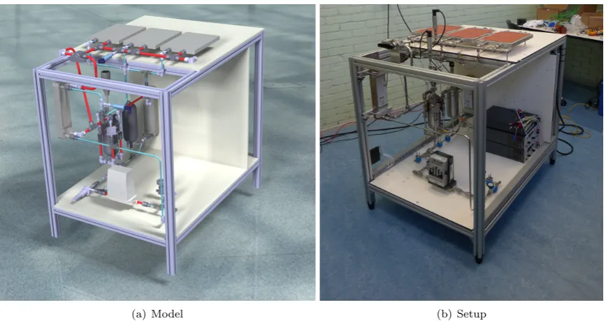
The heat load will be absorbed by the liquid in the evaporators. As a result the liquid will evaporate partially. The two-phase flow that exits the evaporators is now transported to the condenser (see also figure 1), where the fluid condenses to a liquid. Now the liquid can be pumped back to the evaporators. A preheater is being used to increase the temperature of the liquid to near the saturation temperature before it enters the evaporators. A bypass is made in the two-phase flow so the positive influence of this preheater can be proven during tests. The accumulators control the pressure and temperature in the system.

Figure 1: Schematic overview of the two-phase loop

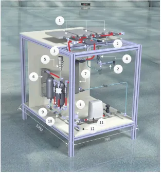
(a) Model (b) Setup

Figure 2: Setup design and actual setup

Steady state modeling

Pressure drop and heat transfer in the cooling of the accumulator is modeled. Two different correlations are used for the two-phase frictional pressure drop (Muller-Steinhagen and Heck, Friedel). Also the minor, gravitational and momentum pressure loss are taken into account. To be able to only apply a certain heat load on two in stead of three evaporators without evaporating all liquid, restriction tubes are designed.

The total pressure drop (figure 3) over the entire loop is approximately 0.7 bar. Approximately 45% of

this pressure drop is caused by the restriction tube and the evaporator and 18% is caused by the heat ex-changers on the accumulator and the corresponding elbows. On the total pressure drop of the entire loop

the difference between the two correlations that are used is±5%. The frictional pressure drop contributes

for more than 50% and the minor pressure loss ±40%. Since there are a lot of elbows in the system, this

is as expected.

(a) Steady state pressure drop along the loop (b) 1D representation of the cooling system

Figure 3

fluids is the same so thermoelectric modules will be used. These modules create a temperature difference between the both side when a power is applied on it. For the convection of the two-phase flow in the cooling channels, four different correlations are used (Yu et al, Kew and Cornwell, Lazarek and Black, Kaew-On et al.). The contact conductance appeared to be a big uncertainty in the model and the different correlation show big differences (figure 4b).

(a) Temperatures in cooling system (Kew and Cornwell)

(b) Performance of different correlations

Figure 4: Heat transfer in the cooling system

Time dependent model

The time dependent model of the NLR was adapted for the use in this project. Some improvements were made and the pressure drop models were inserted. Most results were as expected, only the total pressure drop gave a significant lower value than calculated (0.53 bar).

Conclusions

The 3D model is being used to build the setup and this was very efficient. Improvements were made in an early stage and the installation went smooth.

Steady state calculations are done and uncertainties are determined. The total pressure loss will be around 0.7 bar. Minor pressure loss is of big influence and can not be neglected. The heat transfer calculation show a lot of uncertainties.

The time dependent model is improved and adapted to this project. The pressure drop showed a lot lower result than the steady state calculation. This is probably due to using an other flow model.

Recommendations

Tests should be done to validate the different models. The used pressure drop and heat transfer correlations should be evaluated. Test should be done to find the best flow model for this project.

More research should be done into contact conductance, since this is the biggest uncertainty during modeling.

More improvements should be made in the time dependent model. The heat transfer models should be implemented and the accuracy should be improved and different flow models can be inserted. Besides this a few changes can be made to make to model more user friendly.

Contents

Nomenclature iv

1 Introduction 2

1.1 Background of a Two-Phase Mechanically Pumped Loop . . . 2

1.2 Description of the assignment . . . 2

1.3 General description of the two-phase mechanically pumped loop . . . 2

2 Test setup 4 2.1 Build setup . . . 5

3 Steady state pressure drop 6 3.1 Method . . . 6

3.1.1 Frictional pressure loss . . . 6

3.1.2 Minor pressure loss . . . 9

3.1.3 Gravitational pressure loss . . . 9

3.1.4 Momentum pressure loss . . . 9

3.1.5 Internal geometry . . . 10

3.2 Results calculations . . . 11

3.2.1 Evaporators . . . 11

3.2.2 Restriction for evaporators . . . 11

3.2.3 Entire loop . . . 12

4 Heat transfer calculations (1D) 14 4.1 Heating capacity accumulator . . . 15

4.2 Cooling capacity accumulator . . . 15

4.2.1 Method . . . 16

4.2.2 Numerical results . . . 21

4.3 Heating of the evaporator . . . 25

5 Time dependent model 27 5.1 Creating a stable and accurate model . . . 27

5.2 Improvements model . . . 27

5.3 Results . . . 28

5.3.1 Heat load on all evaporators . . . 29

5.3.2 Heat load on two evaporators . . . 31

6 Conclusions and recommendations 33 6.1 Conclusions . . . 33

6.2 Recommendations . . . 33

Bibliography 34 A Schematic overviews 35 B Data sheets components 38 B.1 Evaporator . . . 38

B.2 Thermoelectric module (Peltier) . . . 39

B.3 Condenser . . . 41

B.4 Preheater . . . 43

1

Introduction

1.1

Background of a Two-Phase Mechanically Pumped Loop

Regular cooling systems use a cooling liquid and are relative large and heavy. By choosing for a two-phase system, the mass of the system will be a lot smaller and also smaller tubing is required, since the latent heat of most fluids is at least one or two orders larger than the sensible heat. For aerospace application this is an important argument. Another big advantage is the temperature stability. A two-phase system uses evaporation to absorb the heat, so the temperature in the evaporator remains constant.

Department ASSP (Space Systems) of the National Aerospace Laboratory develops these kind of cooling systems. Most of the time prototypes are made for costumers and do not stay at the NLR. So for tests for internal use a demonstrator will be made.

1.2

Description of the assignment

Initially the assignment was to make a 3D CAD model with drawings and to model and test the steady state pressure drop and heat transfer in the system. Unfortunately there were a lot of setback during the assembling of the setup. To win some time it was decided to add also assisting in the assembly of the setup. Unfortunately the setup was not assembled in time to do tests.

3D model and setup

Since most decisions about the loop were already made, only the tubing had to be designed during the 3D modeling and drawings had to be made for the assembler. Besides this the electrical circuit (0-36V) was installed and some tubing was done, to speed up the assembling process.

Model of the flow

The pressure drop had to be modeled to determine if the pump was strong enough. Since the NLR does not work very often with R134a (what is chosen for this loop) new correlations for the two phase pressure drop and heat transfer had to be found in literature. Also a model had to be made to predict the heat transfer in the accumulator cooling. There are a lot of ways to cool the fluid in the accumulator. For this loop, thermoelectric modules in combination with heat exchangers are chosen. The maximum heat load on the evaporators had to be found to prevent overheating of the heating foil. Since testing could not be done before the end of the internship, there was time to try to get the already existing time dependent model to work for this setup.

First the setup will be described. Then the steady state pressure drop and heat transfer models will be discussed. Unfortunately these models could not be validated during this internship, but through this there was some time to get some results from the time dependent model. The most result are represented in graphs, but from the results of the time dependent model there are also short movies made. These can be found by clicking on it in the digital version of this report. For better quality it is strongly recommended to download them.

1.3

General description of the two-phase mechanically pumped

loop

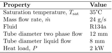
Property Value

Saturation temperature, Tsat 35°C

Mass flow rate, ˙m 24 g/s

Fluid R134a

Tube diameter two phase flow 12 mm

Tube diameter liquid flow 8 mm

Heat load,P 2 kW

Table 1.1: Main specifications and requirements of the system

The heat load will be absorbed by the liquid in the evaporators (see also figure 1.1). As a result the liquid will evaporate partially. The two-phase flow that exits the evaporators is now transported to the condenser, where the fluid condenses to a liquid. Now the liquid can be pumped back to the evaporators. A preheater is being used to increase the temperature of the liquid to near the saturation temperature before it enters the evaporators. A bypass is made in the two-phase flow to prove the positive influence of this preheater. The accumulators control the pressure and temperature in the system. A larger version of the schematic overview can be found in appendix A.

Figure 1.1: Schematic overview of the two-phase loop

Initially there were two three-way-valves at the places marked with TWV ->T. To simplify the tubing,

chosen is to replace this valves by tees and seal the branch which is not used for that test run.

The saturation temperature of the system will be 35°Celsius. Thermodynamic properties of R134a at this

temperature can be found with the database Reference Fluid Thermodynamic and Transport Properties (REFPROP) [1] and are given in table 1.2.

Property Value

Saturation pressure,psat 8.87 bar

Density of the liquid,ρl 1.17·103 kg/m3

Density of the vapour,ρv 43.4 kg/m3

Dynamic viscosity of the liquid,µl 1.72·10−4 Pa s

Dynamic viscosity of the vapour,µv 1.21·10−5 Pa s

Surface tension, σ 6.8 N/m

2

Test setup

A 3d model was created with CAD-program CATIA V5 to visualize the loop and to make drawings, for the manufacturing of the tubing and for assembling. Before this internship assignment started, most part was already thermodynamically designed and a lot of components were already purchased. So for modeling the main issue was the setup design.

Starting points for tubing:

ˆ The pressure drop should be kept as low as possible. This means that the path should be as short

as possible with less elbows, reducing unions and tees. Since a two-phase fluid has more pressure drop than the liquid flow, this flow should have the most efficient path.

ˆ It is very interesting to show the demonstration loop to costumers. The tubing must stay very

straightforward, so the flow is easy to follow.

The visualization showed that the thermodynamical design made the tubing very complex. In this earlier design there were more three-way valves and safety valves, which all required a lot of extra tubing. In the final design this three-way valves are replaced by tees. The branch which is not used will be sealed by a plug fitting. The final setup model is shown in figure 2.1 and a list of the most important components is given in table 2.1.

The numbered items are given below. The available data sheets can be found in appendix B.

Component Type

1 Evaporator Lytron CP 30 (3x)

2 Pressure sensors GE Unik 5000

3 Valves and fittings Swagelok components

4 Burstdisk Schlesinger U20n11-03L

5 Level sensor Sick LFP0300 Inox

6 Condenser Swep B8T M

7 Preheater Swep B8T M

8 DP-sensor Validyne DP 15

9 Accumulator Swagelok 304L HDF4-1000

- Accucooling NLR designed heat exchanger+TE thermoelectric module (4 on one accumulator)

- Accuheating REF max. 200 W (2 on both accumulators)

10 Filter Swagelok SS-8F-K4-140

11 Flowmeter Bronkhorst M5x Cori-Flow

12 Pump NACPA II BBM

Table 2.1: Components and types of the loop

2.1

Build setup

The setup was planned to be finished in beginning of January but eventually the setup was almost ready for testing at the end of February. There were a lot of delays in the delivery of components, but the biggest setback was found in the last stage. During the testing for leaks, a big leak was found in the pump. The first leak was easily fixed, but a new leak was discovered, which could not be sealed at the NLR so the pump (which is also missing in the picture) had to be send back to the manufacturer.

(a) Model (b) Setup

Figure 2.2: Setup design and actual setup

3

Steady state pressure drop

The total pressure drop determines the pressure rise the pump has to achieve. A pump is bought assuming a pressure rise of approximately 1 bar. Steady state pressure drop calculations are done to confirm this order of magnitude. R134a is not often used at the NLR, so different models are used and should be validated so the best model is known for future design.

3.1

Method

The total pressure drop consists of different components: the frictional pressure loss, minor pressure loss, gravitational and momentum pressure loss respectively:

∆ptotal= ∆pfric+ ∆pmin+ ∆pgrav+ ∆pmom (3.1)

For systems with long tubes, the frictional pressure loss will be the major part, but for systems with a lot of elbows and other disturbances, the minor pressure loss can become quite large. For vertical tubes the gravitational pressure change is calculated and for components where large velocity changes take place the momentum pressure loss should be taken in to account. An approximation is done by assuming that

the fluid in the entire loop is at the satuartion point with a temperature of 35°C.

3.1.1

Frictional pressure loss

The frictional pressure drop of a two-phase flow can be calculated from the pressure drop of the single-phase pressure drop of a liquid flow and a vapour flow. First the mass fraction of the two-single-phase flow has

to be determined. The heat load (Pin) causes the liquid in the evaporator to (partially) evaporate. This

means that the vapour mass fraction in the evaporator will increase from 0 to x. This increase can be

calculated with:

∆x= Pin

˙

m hlv

(3.2)

Withhlv, the specific latent heat of vapourisation.

Frictional pressure drop of a single-phase flow

The frictional pressure drop for a liquid and vapour flow respectively is calculated with the Darcy-Weisbach equation (C¸ engel and Ghajar 2011 [2]):

∆pl,fric=fl

L d

ρlv2l

2 , ∆pv,fric=fv

L d

ρvv2v

2 (3.3)

The friction functionf is calculated different for different Reynolds numbers. The equations are given for

the liquid case and are similar for the case of a vapour flow. The Reynolds number is calculated with:

Rel =

ρld vl

µl

(3.4)

vl =

˙

m

ρπd2_/4 (3.5)

For laminar flows in a tube, the friction coefficient is given by (C¸ engel and Ghajar 2011 [2]):

fl= 64/Rel laminar f low(Re <2400) (3.6)

And for turbulent flow an empirical equation is found by Colebrook and White 1937 [3]:

1 √

fl

=−2 log₁₀

_/d

3.7 + 2.51

Rel √

fl

This implicit equation can be approximated by the explicit Haaland equation (C¸ engel and Ghajar 2011, Romeo et al. 2002 [2, 4]):

1 √

fl

=−1.8 log₁₀

_/d

3.7

1.11

+ 6.9

Rel

turbulent f low(Re >4000) (3.8)

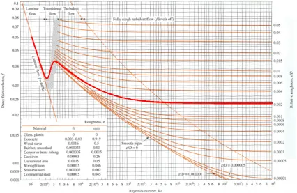
The results of this approximation are within 2 percent of those obtained from the Colebrook equation. Since there are a lot of bigger uncertainties (like the geometry of the components), this is not a problem.

Figure 3.1: Moody diagram

The analytical value of the friction factor and the one from the Colebrook equation can be plotted in a

moody diagram (C¸ engel and Ghajar 2011 [2]). In the transition region (2400< Re <4000) the flow can

be turbulent, laminar or something in between. From the Moody diagram (figure 3.1) it becomes clear that there is a jump in the graph in the transition region. To get a accurate solution it is important to know the place of the jump. This is not easy to find and the experience at the NLR is that in reality there

is no jump (Ghajar and Madon 1992, C¸ engel and Ghajar 2011 [5, 2]). To let this have a small influence

on the results, a smoothing function is used between the laminar and turbulent friction factor:

ζ= 1

1 +exp(−(Rel−2400)/200)

(3.9)

fl= (1−ζ)fllaminar+ζfvturbulent (3.10)

Frictional pressure loss of a two-phase flow

There are a lot of correlations known to predict the frictional pressure drop of a two-phase flow. Research is done by Kim and Mudawar (2013)[6] which correlation works best for mini/micro-channel boiling flows with different thermodynamic and geometric parameters. The evaporation takes place in mini-channel, as can be seen in figure 3.2.

Figure 3.2: Interior of one of the evaporators

For the evaporator the most accurate relations where found by comparing the results of the relations with data-points of the databases with more or less the same parameters. Since a lot of parameters influence the pressure drop it is hard to find exactly the same case. The fluid, diameter of the channels and the mass flux are assumed to have the biggest influence. The Muller-Steinhagen and Heck relation and the Friedel relation appear to be a good approximation (Kim and Mudawar (2013)[6]).

ˆ Muller-Steinhagen and Heck relation

∆ptp,fric(x) = (∆pl+ 2(∆pv−∆pl)x)(1−x)1/3+ ∆pvx3 (3.11)

ˆ Friedel relation

∆ptp,fric(x) = ∆pl

A+ 3.43B

F r0.047 l W e

0.0334 l

(3.12)

withA = (1−x)2+x2

_ρ l ρv _f v fl

B = x0.685(1−x)0.24

_ρ l

ρv

0.8_µ v

µl 0.22

1−µv

µl 0.89

F rl =

G gdρl

, W el=

Gd ρlσl

3.1.2

Minor pressure loss

There are different flow models which can be used, to make two-phase flow calculations of the minor pressure loss, gravitational pressure loss and the momentum pressure loss less complex. Two often used models are the homogeneous flow model, where the liquid and vapour stream are assumed to have the same velocity and the separated flow model where the two phases are modeled as two flows (liquid and vapour) trough separate tubes with corresponding area. The homogeneous flow model is less complex than the separated flow model, but also a lot less accurate (Kim and Mudawar 2013 [6]). Therefore, the separated flow model is used.

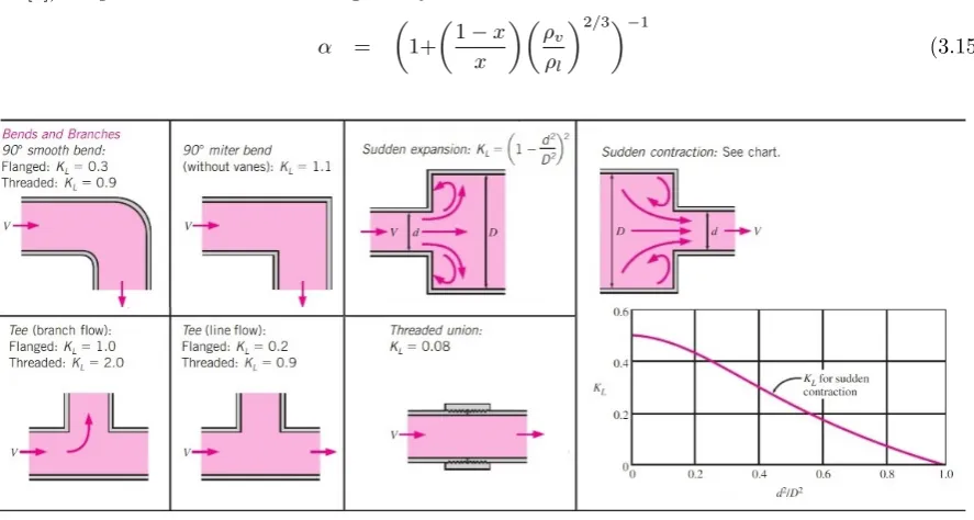
Minor losses are the losses due to interruptions of the smooth flow of the fluid. For systems with long tubes these losses are minor, but for systems with a lot of components as elbows, tees and unions, the minor losses may be larger than the major losses. The minor pressure loss is given by (Munson et al. 1990, C¸ engel 2012 [7, 8]):

∆ptp,min = Kl

1 2ρtpv

2

tp (3.13)

ρtp = (1−α)∗ρl+α∗ρv (3.14)

With Kl, the loss coefficient. In figure 3.3 the loss coefficient is given for different components (C¸ engel

2012[8]). Vapour volume fractionαis given by Zivi’s correlation:

α =

1+

_1−x

x

_ρ

v

ρl

2/3−1

(3.15)

Figure 3.3: Minor loss coefficient for different components

3.1.3

Gravitational pressure loss

In vertical tubes the pressure changes through gravity. This change is given by (Kim and Mudawar 2013 [6]):

∆ptp,grav = sin(φ)ρtpg∆z (3.16)

3.1.4

Momentum pressure loss

In the evaporator and condenser the density and thus also the velocity changes. This change in the momentum results in a pressure change to keep conservation of momentum. In the evaporator this will be a pressure drop and in the condenser the pressure increases.

∆ptp,mom = _ρ

tpvtp2

2

out −

_ρ tpvtp2

2

in

3.1.5

Internal geometry

The internal geometry of the evaporators should be known to be able to perform accurate calculations. A graph of the pressure drop for water is available (see figure 3.4a). With this information and the database REFPROP [1], the pressure drop can be calculated for R134a. Since the frictional pressure drop is a function of the Reynolds number, it is not accurate to just assume one tube with dimensions that result in the same pressure drop for water. So the number of tubes and the dimensions should be approximated and tweaked to get the same pressure drop. Figure 3.2 is used for a first approximation.

As can be seen in figure 3.4a it is possible to approximate the pressure drop for water by using different geometries. But when the fluid and temperature change (figure 3.4b) it is clear that the two possible solutions are not the same. In table 3.1 the different geometries are given.

(a) For water at 20°C (b) For R134a at 35°C

Figure 3.4: Pressure drop as function of the flow rate. Geometries of the two approximations are given in table 3.1

Length tube(s) Diameter tube(s) Number of parallel tubes

Blue 48 cm 0.9 mm 38

Red 2,5 cm 1.92 mm 1

Table 3.1: Geometry parameters of the two approximations

The ”blue geometry” is constructed using the picture from the manufacturer and should be the best approximation.

3.2

Results calculations

3.2.1

Evaporators

The pressure drop is a function of the mass vapour fraction. In figure 3.5 the pressure drop over the evap-orators is plotted as a function of the mass vapour fraction at the end of the evaporator. In the evaporator the mass vapour fraction increases trough the evaporation of a part of the liquid. The assumption is made that the mass vapour fraction increases linear over the length of the tubes. For a heat load of 2kW, the mass vapour fraction at the exit will be 0.496.

Figure 3.5: Pressure drop as function of the mass vapour fraction at evaporator exit

3.2.2

Restriction for evaporators

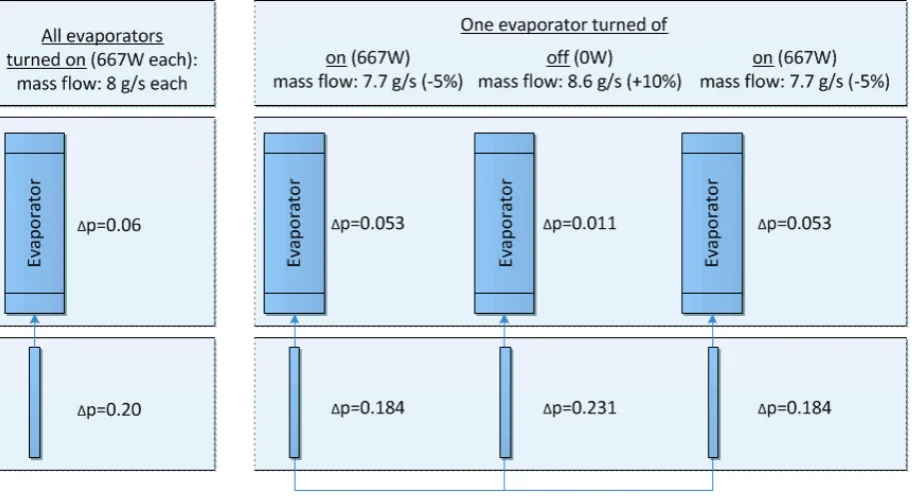
The three Lytron evaporators are placed parallel. This has the big advantage that there is less pressure drop. But it has also a downside. When one of the evaporators is turned off the flow will take the path with the least resistance, which is through the evaporator which is turned off. So the mass flow trough the evaporator which is turned off increases until the pressure drop over the branches is the same and the mass flow trough the other two evaporators decreases. Calculations make clear that this decrease is huge: the mass flow rate in the working evaporators will decrease 40% (see also figure 3.6) when one evaporator is switched off.

Now only 42% of the mass flow goes trough the working evaporators. Using equation 3.18 the mass fraction of the two-phase flow can again be calculated. The vapour mass fraction will increase from 0.50 to 0.79. When the two evaporators which are turned on absorb a heat load of 667W each before and 1kW each after one evaporator is switched off (so the same total heat load), the vapour mass fraction will increase from 0.5 to 1.33. Since the mass vapour fraction is maximum one for vapour, this is not possible. So or a lower heat load is accepted or fluid with a higher temperature will travel through the system and all advantages of a two-phase loop are undone.

∆x= Pin

˙

m hlv

(3.18)

To prevent this from happening and to be able to meet the requirements a restriction is made in the tube before the evaporator in such a way that the pressure drop in this tubes is higher than the pressure drop inside of the evaporators. In this way there is less influence of changes in the performance of the evaporators. When a tube with a length of 60 mm and an inner diameter of 1.5 mm is placed in the front of the evaporator the total pressure drop in the parallel branches is approximately 0.25 bar (see also figure 3.7). The pressure drop of an evaporator is only 0.06 bar (when all three are turned on), so when one evaporator is turned off this results in a drop of mass flow in the working evaporators of only 10 percent. This is acceptable, since the vapour mass fraction then increases from 0.50 to 0.52 in the working evaporators the applied heat load is 667 W each and from 0.5 to 0.81 when the total heat load stays 2kW.

Figure 3.7: Pressure drop in the evaporators using restriction tubes (bar). Correlation: Friedel

When Muller-Steinhagen and Heck is used, the result is that the vapour mass fraction increases from 0.5 to 0.52, for the case where on evaporator is switched off and the heat load per evaporator is 667 W. So the difference is small.

3.2.3

Entire loop

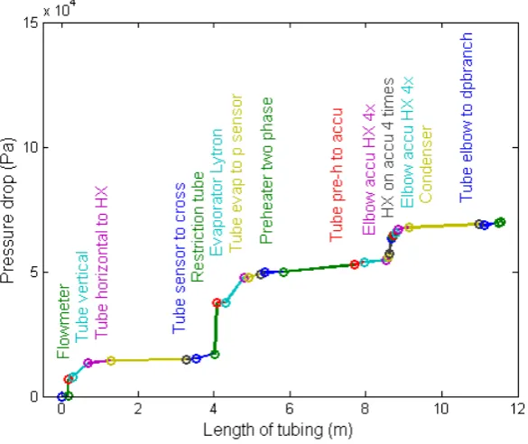
From figure 3.8 it becomes clear that there are a few points were the total pressure drop increases rapid. Only the names of parts where the pressure drop increases with more than 0.01 bar were printed in the graph. Soon after the pump there are two tubes with high pressure drops, a long vertical tube (mainly gravitational loss) and a long horizontal tube (mainly frictional loss). Further on indeed the restriction tube and evaporator contribute a lot and a third big jump can be found due to the heat exchangers on the accumulator (HX on accu). This losses are mainly caused by the minor losses in the elbows and the frictional losses in the small inner tubes of the heat exchangers.

Figure 3.8: Cumulative pressure drop in the loop using Friedel correlation

The total pressure drop over the entire loop is approximately 0.7 bar. Approximately 45% of this pressure

drop is caused by the restriction tube and the evaporator and 18% is caused by the heat exchangers on the accumulator and the corresponding elbows. Since two different correlations are being used to calculate the frictional pressure loss, it is interesting to see what the difference is in the total pressure drop. The biggest differences are found for the evaporators and the heat exchangers on the accumulator (table 3.2).

On the total pressure drop of the entire loop the difference is±5%.

∆ptotal using Muller-Steinhagen ∆ptotalusing Difference

and Heck correlation Friedel correlation

Evaporator and restriction 3.06·104_{Pa 2.81·10}4 _{Pa 2.5·10}3_Pa

Heat exchangers

on accumulator (4x) 1.26·104_{Pa 1.18·10}4 _{Pa 8.2·10}2_Pa

Loop 6.94·104_{Pa 6.58·10}4 _{Pa 3.6·10}3_Pa

Table 3.2: Pressure drop using different correlations

It is also interesting to know how much the different kind of pressure drops contribute to the total pressure

drop. The frictional pressure drop contributes for more than 50% and the minor pressure loss±40%. Since

4

Heat transfer calculations (1D)

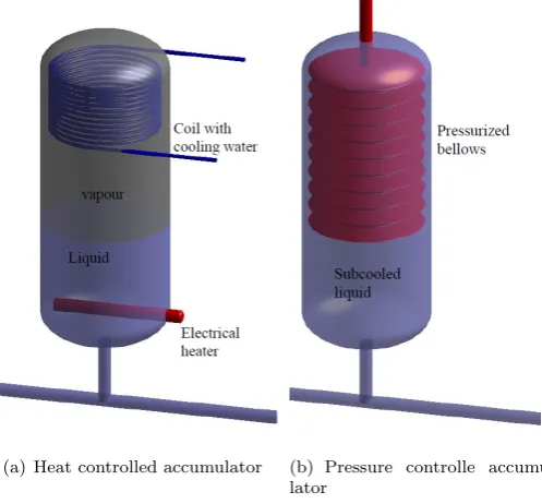
When the heat load changes, the amount of liquid per time unit that is evaporated changes also. This means that the vapour mass fraction will change and as a result also the density. Liquid will now flow in or out of the accumulator and the pressure and temperature in the accumulator and in the entire system will also change. A two-phase mechanical pumped loop is usually used when a uniform system temperature is required. An accumulator is being used to control the pressure in the loop in order to return to the desired temperature. Two types of accumulators are possible; Heat Controlled Accumulators and Pressure Controlled Accumulator (see figure 4.1). Heaters can evaporate a part of the liquid on the bottom of the accumulator to increase the pressure and when the pressure should decrease the top of the accumulator is cooled.

(a) Heat controlled accumulator (b) Pressure controlle accumu-lator

Figure 4.1: Two types of accumulators

4.1

Heating capacity accumulator

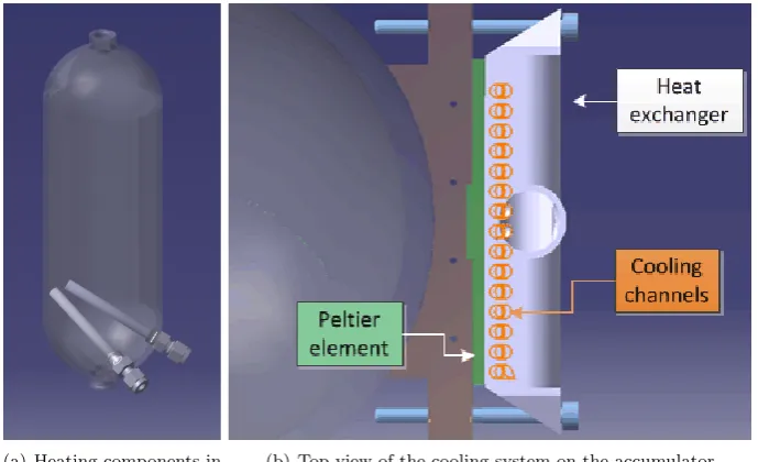
Heating can be done in different ways, for example by soldering heat exchangers on the accumulator wall or by using electrical heaters. In this loop heating is simply done by two electrical heaters at the bottom of the accumolators as can be seen in figure 4.2a.

All heat will be transferred into the liquid, as long as the heaters do not get overheated. So when the heaters are turned on, it is known how much the cooling system needs to cool to undo the heating.

(a) Heating components in the accumulator

(b) Top view of the cooling system on the accumulator

Figure 4.2: Cooling and heating in the accumulators

4.2

Cooling capacity accumulator

There are also different methods to cool the vapour in the top part of the accumulator. In short they can by divided in two groups: systems which cool the liquid directly and systems which cool the accumulator wall. Chosen is to use heat exchangers to cool the wall of the accumulator. The sub-cooled liquid flow or the two-phase flow can be used as cooling fluid. Since the liquid has to stay liquid and therefore can not be heated up much, the two-phase flow is used. This flow can absorb a lot heat without heating up but the problem is that this flow has the same temperature as the two-phase flow in the accumulator, so a temperature difference should be generated. This is done by using thermoelectric modules. In the thermoelectric modules, electrical energy will be used to transport the heat from one side to the other side (the Peltier effect). In this way, one side will become a cooling plate. The cooling system is illustrated in figure 4.2b.

4.2.1

Method

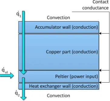
The cooling system is approximated by the 1D model in figure 4.3. The model is further simplified by assuming that there is no heat transfer out of the system. The temperatures at all interfaces are calculated and the temperatures on both ends are known (saturation temperature). The resistance components up to the thermoelectric module (Peltier) are calculated using the heat transfer rate caused by the heater. The heat transfer after this module also depends on the electrical power of the module.

Figure 4.3: 1D approximation of the cooling system on the accumulator

Conduction

Conduction takes place in the accumulator wall, the copper part and heat exchanger wall. The heat transfer due to conduction is calculated using the general heat conducting equation (Fourier-Biot) and

Fourier’s law (C¸ engel and Ghajar 2011 [2]). For a steady 1D situation without heat generation this

becomes:

qcond = −k

(T1−T2)

dx (4.1)

WhereT1andT2 are the surface temperatures, as illustrated in figure 4.4

Figure 4.4: Conduction through a wall

Thermal conductivity k changes with the temperature. Since the temperature distribution through the wall is linear, the average temperature can be taken to find the value of the thermal conductivity. The temperatures in the system are different for different heat transfer rates, so it is not perfectly accurate to use a constant. But for the used metals the thermal conductivity changes only a few percent over our temperature range. More uncertainty is caused by not knowing exactly the composition of the copper alloy and the titanium alloy for the heat exchanger. The heat exchangers are 3D printed. This would influence the thermal conductivity also, because of the anisotropy in the material. Since temperature differences are not of big influence on the thermal conductivity, the thermal conductivity is used at 300 K (kstainless steel= 15W/mK, kcopper= 150W/mK , ktitanium= 21.5W/mK, kaluminium= 170W/mK).

Convection

Convection takes place from the two-phase fluid to the accumulator wall and from the heat exchanger wall to the two-phase fluid. The rate of convection heat transfer is given by Newton’s law of cooling:

qconv=−h(Ts−Tsat) (4.2)

Where Ts is the temperature of the surface and Tsat the temperature sufficiently far from the surface.

Heat transfer coefficient h is different for the two convection heat transfers in this system.

In the accumulator there is condensation on a vertical wall. The average heat transfer coefficient for

laminar film condensation over a height L is determined to be (C¸ engel and Ghajar 2011 [2]):

hvert =

4 3

_gρ

l(ρl−ρv)h∗lvk 3 l

4µl(Tsat−Ts)L 1/4

(4.3)

h∗_lv = hlv+ 0.68cp,l(Tsat−Ts) (4.4)

For the convective heat transfer in the heat exchanger a lot correlations can be found for the heat tranfer coefficient. To find the most suitable correlation for R134a in mini-channels, literature is found where the performance of the correlations is compared for different experimental datasets (Qu and Mudawar 2003, Kaew-On et al. 2011, Ong and Thome 2011 [9, 10, 11]). From different studies, a few correlations appear to perform well and are chosen to calculate the heat transfer.

ˆ Lazarek and Black

htp= 30Re0.857l Bo 0.714kl

d (4.5)

ˆ Kew and Cornwell (Modified Lazarek and Black)

htp = 30Re0.857l Bo0.714

kl

d(1−x)

−0.143 _(4.6)

ˆ Yu et al.

htp= 6.4·106(Bo2W e)0.27

ρl

ρv −0.2

(4.7)

ˆ Kaew-On et al.

htp = SBo0.185W e0.0012hl (4.8)

With: S = 1.737 + 0.97(βφ2_l)0.523 (4.9)

φ2_l = 1 + C

X +

1

X2 (4.10)

C = −3.356 + 41.83eA+B (4.11)

A = −17.369fld (4.12)

B = 124.5fld (4.13)

X =

_f l

fv 0.5

(1−x)

x _ρ v ρl 0.5 (4.14) With:

Bo = q˙

Ghlv

(4.15)

hl = 0.023Re0.8l P r 0.4 l _k l d (4.16)

W e = G

2_d

ρlσ

Thermal contact conductance

On both sides of the thermoelectric module a thermal contact resistance is present. Heat is transfered in this contact through conduction where the materials make contact and through radiation and convection through the air in between the parts. The temperature differences can be calculated in an analogous

manner to Newton’s law of cooling (C¸ engel and Ghajar 2011 [2]):

qcontact=−hc(T1−T2) (4.18)

With the contact conductancehc. This contact conductance depends on the roughness, the materials of

the parts, the medium between the two materials and contact pressure. C¸ engel [2] stated thathc usually

has a value between 2000 and 200000 W/(m2K). The worst case scenario is a stainless steel contact with

a hc of 2000 W/(m2 K). Since the exact material properties of the used contact materials are unknown,

the stainless steel contact is used as worst case scenario. Correlations are developed which can be used to find the contact conductance.

Contact resistance is only present in the contact on both sides of the thermoelectric module. High contact pressure is applied on these surfaces using a screw connection with bolting washers. Due to this high pressure the surfaces will deform plastically and therefore a plastic model is used. Since the exact material properties are unknown, the Cooper, Mikic and Yovanovich (CMY) correlation will be the most suitable (Sridhar and Yovanovich 1994 [12]). In the CMY model (Cooper et al. 1969 [13]) the dimensionless

contact conductanceCc is a function of the dimensionless pressure (p/Hc):

Cc =

1

2√2π

exp(−λ2_/2)

1−

q

1/2erf c(λ/√2)

1.5 (4.19)

λ = √2erf c−1

2 p

Hc

(4.20)

This model is valid for (p/Hc) : 10−6−10−2.

Since the order of magnitude of the contact pressure is known by knowing the maximum pressure which can

be applied on the bolting washers, the contact conductancehc can be found for this pressurep(Song and

Yovanovich 1988, Sridhar and Yovanovich 1996 [14, 15]). Therefore the pressure and contact conductance should be written as a function of the dimensionless numbers.

hc = Ccks

m

σ (4.21)

p Hc

=

_p

c1(1.62·106_mσ)c2

1+0.1071c2

(4.22)

For stainless steel: c1= 6.271·106 ,c2=−0.229 [15]. The only uncertainty is _mσ. Typical values are _mσ:

8 µm- 60µm. The thermal contact conductance is plotted for this values in figure 4.6.

Figure 4.6: Contact conductance for the pressure

The pressure on the surface will be of order 105Pa. The CMY model isn’t validated for that pressure, but

when is assumed that the trend will continue for pressures untill 105Pa, the thermal contact conductance

Thermoelectric cooling

To test the performance of the cooling system the heaters will be turned on with a known power. When the cooling system is turned on and steady state is reached, it is known that the cooling power is equal to the heating power. The performances curves of the thermoelectric cooling module are given by the manufacturer (figure 4.7). This data is interpolated to get more data-points. In the left hand side figure, the current is found for a needed cooling power and temperature difference and then the voltage and therefore also the needed electrical power is found in the graph on the right hand side. The heat transfer rate on the hot side of the thermoelectric module is the cooling heat transfer rate plus the electrical power. Since the heat transfer rate after the thermoelectric module depends on the electrical power, an iteration is done to get zero temperature difference over the entire system. The temperature difference should be zero since the temperature of the two phase flow is more or less the same in the entire loop. Note that

the used performance data in the data sheet is only specified for a hot side of 25°C. However, there is no

information given by the manufacturer to convert this to the right temperature.

4.2.2

Numerical results

The temperatures over the system are plotted like figure 4.8 for different correlations and cooling powers. The mentioned cooling power is the needed cooling power per cooling unit. The temperature on the beginning and end (two phase flow) is the same, as it should be. The first temperature drop is due to the condensation film on the inside of the accumulator. The biggest temperature difference due to conduction is in the accumulator wall. The contact resistances between the copper part and thermoelectric module is not of big influence. But the contact resistance between the thermoelectric module and the heat exchanger (HX) can be of big influence, especially for high cooling powers (e.g. 57,5W see figure 4.9). In that case the heat transfer rate at the hot side of the thermoelectric module will be much larger than at the hot side.

Figure 4.8: Temperatures in all components. Correlation: Kew and Cornwell, Cooling power: 40W

When the electrical power increases, the cooling power will also increase, but the coefficient of performance (cooling power divided by electrical power) will decrease. So there will be a maximum cooling power. The founded values for the electrical en cooling power are plotted in figure 4.10a by the solid line. For lower and higher values of the cooling power, no data is available from the manufacturer. The higher and lower values are found (dashed line in figure 4.10a) by assuming that the coefficient of performance is linear (figure 4.10b). When the electrical power is increased further than the maximum, the cooling power will decrease and eventually extra heat is transferred into the system (see figure 4.11).

(a) (b)

Figure 4.10: Performance of the thermoelectric component. On the right the approximation for the COP that is used Correlation: Kew and Cornwell

The performance can also be seen in the diagram of the cooling power as function of the temperature

difference (figure 4.12). The data given by the manufacturer (figure 4.7) is interpolated (for I= 3 : 0.1 :

15.4 A) and the cooling power and temperature differences of our system is plotted. Again the solid line

is the result from a simulation and the dashed line is the result of the extrapolation. More data-points were available for bigger temperature differences, but for these points the temperature drop of the system increased faster than the temperature increase in the thermoelectric module, so the simulation did not converge. The extrapolation in figure 4.12 is more accurate than the extrapolation in figure 4.10, but in the experiments the cooling power and electrical power are known so this will be plotted further on.

Figure 4.12: Cooling power as function of the temperature rise. Correlation: Kew and Cornwell

As said before estimates are done for the thermal conductivity and a worst case scenario is used for the contact conductance. The thermal conductivity of all components could be about 10% higher or lower. In figure 4.13 can be seen that the influence of a change thermal conductivity does not have a very big influence. A big influence is a change in contact conductance. The contact conductance could in reality easily be ten times larger. When the minimum contact conductance multiplied by 5 is plotted, there is already a big difference (see the purple line in figure 4.13).

Different correlations are being used to model the heat transfer in the heat exchangers on the accumulator. As can be seen in figure 4.14 they differ a lot. It is clear that Yu et al. and Kaew-On et al. give a different solution than the other two.

Figure 4.14: Cooling power as function of the electrical power for all used correlations

From the above graphs it can be concluded that is difficult to accurately predict the heat transfer in the cooling system. The biggest uncertainties are the contact conductances from the copper part to the thermoelectric module and from thermoelectric module to the heat exchanger wall and the convection in the heat exchanger. Beside this uncertainties the assumption is done that the thermoelectric module

4.3

Heating of the evaporator

To simulate the heat load on the evaporator, heating foil is placed on the evaporators. The maximum power per heater should be found, to prevent overheating. Given is the graph in figure 4.16a. The maximum power, with PSA as mounting method (blue line in figure 4.16a), per effective area is converted to the maximum power per evaporator. Heat is transferred trough convection from fluid to evaporator wall, conduction in the evaporator wall and there is a contact resistance between the heater and the evaporator. Since the maximum power is given for different mounting methods, assumed is that contact resistance is included in figure 4.16a. Now the thermal resistances are given in figure 5.2. An initial guess is made of the maximum power. With this power, the heat sink temperature is calculated using the earlier given heat transfer relations (equation 4.1- 4.17). For one phase heat transfer the heat transfer coefficient

for developing turbulent flow can be calculated with (C¸ engel and Ghajar 2011 [2]):

h = N u kl

d (4.23)

with: N u = 0.023Re0.8P r0.4 , P r=µcp

kl

(4.24)

With the given maximum power per effective area, the maximum power for our system is found using an iterative procedure. For an initial power input the heat sink temperature is calculated. For this temperature the maximum power is found in the graph. This power is used as new input for the iteration. Since the spiral diverged, the difference between the old input power and new input power is damped. In figure 4.16b, the iteration process using a damping factor of 0.7 is plotted.

(a) Given maximum heat load (b) Calculated maximum heat load (damping 0.7)

5

Time dependent model

A time dependent (matlab) model is already present at the NLR. This model is being used to simulate the time dependent behaviour of the loop. In the model the (simplified) enthalpy equation and the mass equation are solved. The MacCormack predictor-corrector scheme (equation 5.1-5.3) is being used to discretize the enthalpy equation and the mass equation is discretized using a forward difference scheme (equation 5.4). Since an existing model is used, a detailed description is not given. For future assignments, students can find more information about the model in the NLR report [16].

H_ip = Hin−uni(Hin−Hin−1)

∆t

∆x+

Qn_i ρn i

∆t −> predictor step (5.1)

H_ic = H_in−un_i(H_i+1p −H_ip)∆t

∆x+

Qn i

ρp_i(H_ip, pn i)

∆t −> corrector step (5.2)

H_in+1 = H_ip+H_ic (5.3)

un+1_i+1 = un+1_i −u n+1 i

ρn+1_i (ρ

n+1 i+1 −rho

n+1 i ) +

(ρn+1_i −ρn_i ρn

i

∆x

∆t (5.4)

The pressure drop and heat transfer models of previous chapters can be inserted in this model with some small changes. For stability a smoothing function is used for the pressure drop. The mean flow speed is calculated so the homogeneous flow model is used. In the simulations, the accumulator cooling is turned on the entire time and the accumulator heating is PI controlled. The Muller-Steinhagen and Heck relation is used for calculating the pressure drop.

5.1

Creating a stable and accurate model

To create some output a few steps have to be taken. First the input has to be correct. The geometry is approximated and loss coefficients and thermal masses are inserted. For the pressure drop the matlab files created for the steady state situation are adapted to the existing model and inserted. The old model only calculated the frictional pressure drop, but in the steady state calculations it was concluded that this is inadequate for this system. The output properties can be plotted over the geometry, so the geometry is adapted in the plot function as well. This was first a 2D function and is improved to a 3D function. The approximation of the geometry is found in figure 5.1. The heat transfer is initially just a constant which is estimated. To get a stable solution the number of element are chosen. Unfortunately it was not easy to get a stable and functioning model, therefore it took a lot of time.

5.2

Improvements model

Some parts of the model work very intuitive and some do not. A few variables could not be changed in the mainfile, therefore you would have to search for them in all function files. Besides that, the components (tubes, condenser e.d.) have names that depend a lot on the geometry. So for every new project the component names in the entire model would have to be changed. Even though it was not initially part of the assignment some improvements are made: the input is made easier, the component names are generalized and there is a brief instruction how to write the geometry input file in such a way that not all files will have to be changed. Besides this, the pressure drop correlation can now be chosen in the mainfile.

(a) Geometry (b) Approximated geometry

Figure 5.1: Approximation of the geometry

5.3

Results

Two simulations are described here. In the first simulation all evaporators are absorbing the same amount of heat. The time dependent behaviour after turning on the heat load is discussed. Besides this, the pressure drop is compared with the steady state calculations. In the second simulation the heat load is only applied on two evaporators. The accuracy of the model can be represented by the conservation of mass. By dividing the mass error by the time step, the difference in mass flow is found.

Figure 5.2: Temperatures in all components for the maximum power

5.3.1

Heat load on all evaporators

Time dependent behaviour

In the figures in figure 5.3 it can be seen how the system behaves when it is switched on. After one minute a heat load of 1kW is applied on the evaporators (figure 5.3a). First the evaporators warm up the fluid until it reaches the boiling temperature (figure 5.3b). Due to the heat exchanger the fluid at evaporator inlet becomes hotter also. After approximately 3 minutes the fluid starts to boil in the evaporator. In the first few minutes a lot of energy is being used to warm op the heat exchanger itself and the liquid flow to saturation temperature as can be seen in the difference in vapour mass fraction of the heat exchanger and condenser (figure 5.3c). Since the density of the two phase fluid will be a lot lower, the mass flow increases locally and will force the fluid to flow into the accumulator (figure 5.3d). When for the first time two phase flow will leave the heat exchanger, the mass flow will increase again. When all evaporators are turned off, the vapour mass fraction will decrease and therefore liquid will flow out of the accumulator.

(a) Power heating and cooling elements (b) Temperature

(c) Vapour mass fraction (d) Mass flow

Figure 5.3: Solution time dependent model, heat load 2kW on three evaporators

Pressure drop

taken into account. In the entire model the pressure drop is about 20 percent off. There are two big differences in the models. In the steady state calculations the temperature in the loop is assumed to be 35 degrees, whereas the temperature in the transient model is calculated every time step for all elements. This seems to be a big overestimation, but when is assumed that in the entire system the temperature

is at a constant value of the maximum temperature (37.7 °C), the pressure drop is still 0.68 bar (using

MSH). So the change is probably not caused by this assumption. The second difference is the flow model: the steady state model uses the separate flow model and the transient model uses the homogeneous flow model. But this also just gives a slightly different answer. So the reason for the different pressure drop is not yet found.

(a) Pressure along the loop at t=15min (b) Pressure drop over time

Figure 5.4: Solution time dependent model, heat load 2kW on three evaporators

(a) Steady state pressure drop (b) Time dependent model, pressure drop

Figure 5.5: Differences in pressure drop

Figure 5.6: Screen shot of the short movie, click to watch

5.3.2

Heat load on two evaporators

(a) Mass flow in the evaporators (b) Pressure along the loop at t=15min

(c) Vapour mass fraction

Figure 5.7: Solution time dependent model, heat load 2kW on two evaporators

6

Conclusions and recommendations

6.1

Conclusions

The setup is drawn in Catia V5 and with the drawings the setup is build. Earlier, the design before making the 3d CAD model was not completly developped. So a lot of changes were made during building the setup. Making good drawings before manufacturing has proven to be efficient: Improvements were implemented a lot easier and the installation went smooth. Also for decision-making it is very useful that everybody has the same geometry in mind. For this reason Catia V5 known how is passed on.

The steady state pressure drop is modeled using two different correlations for the frictional pressure drop: The Muller-Steinhagen an Heck relation and the Friedel relation. The differences between the models were

small. The minor losses are of big influence of the pressure drop (±40%) and can therefore not be neglected.

The steady state heat transfer of the cooling loop is modeled using different methods for the heat transfer coefficient in the two-phase flow. The differences between the models and the uncertainties in the approx-imations were large. The maximum heat load that can be applied on the evaporators is found. This is a lot higher than the range used for testing.

The time dependent model of the NLR is being used to model the time dependent behaviour of the loop. The steady state pressure drop showed a much lower result. This is probably caused by using the wrong flow model. Some improvements are made in the model to make the model easier to use and the two used correlations for the steady state pressure drop are also implemented.

6.2

Recommendations

Since having a 3D model in the beginning of a project has so many advantages it is strongly recommended that there will be more experience of 3D drawing in the thermal group.

It should be tested if the pressure drop models are accurate for the macro channel flow (most part of the loop) and micro channel flow. Since the internal geometry of the heat exchanger on the accumulator and restriction tubes are know, these should be the first component were conclusions are drawn about. When the models are accurate for the heat exchangers on the accumulator and the restriction tubes they will probably also be for the evaporator and then there can be drawn conclusions whether the internal geometry is estimated accurate or not.

Since the contact conductance is so uncertain, more research should be done to this topic. Further, test should be done to check the thermal resistances in the cooling system on the accumulator. Since it is not possible to put temperature sensors between the components it will be very hard to find which correlation for the heat transfer coefficient performs best.

A few improvements can be done in the time dependent model:

ˆ Since the mass flow error was significant, different integration schemes should be considered

ˆ Heat transfer models should be implemented for all components

ˆ The cooling model should be implemented

ˆ Tests should be done to find the best working flow model for this situation and if necessary the

separate flow model should be implemented

Bibliography

[1] E. Lemmon, M. Huber, and M. McLinden, “Nist standard referencedatabase 23: Reference fluid thermodynamic and transport properties-refprop. 9.0.,” 2010.

[2] Y. A. C¸ engel and A. J. Ghajar,Heat and mass transfer: fundamentals & applications. McGraw-Hill,

2011.

[3] C. Colebrook and C. White, “Experiments with fluid friction in roughened pipes,”Proceedings of the

royal society of london. series a, mathematical and Physical sciences, pp. 367–381, 1937.

[4] E. Romeo, C. Royo, and A. Monz´on, “Improved explicit equations for estimation of the friction factor

in rough and smooth pipes,”Chemical engineering journal, vol. 86, no. 3, pp. 369–374, 2002.

[5] A. J. Ghajar and K. F. Madon, “Pressure drop measurements in the transition region for a circular

tube with three different inlet configurations,”Experimental thermal and fluid science, vol. 5, no. 1,

pp. 129–135, 1992.

[6] S.-M. Kim and I. Mudawar, “Universal approach to predicting two-phase frictional pressure drop

for mini/micro-channel saturated flow boiling,” International Journal of Heat and Mass Transfer,

vol. 58, no. 1, pp. 718–734, 2013.

[7] B. R. Munson, D. F. Young, and T. H. Okiishi,Fundamentals of fluid mechanics. New York, 1990.

[8] Y. A. C¸ engel,Fundamentals of Thermal-Fluid Sciences. McGraw-Hill, 2012.

[9] W. Qu and I. Mudawar, “Flow boiling heat transfer in two-phase micro-channel heat sinks—-i.

experimental investigation and assessment of correlation methods,” International Journal of Heat

and Mass Transfer, vol. 46, no. 15, pp. 2755–2771, 2003.

[10] J. Kaew-On, K. Sakamatapan, and S. Wongwises, “Flow boiling heat transfer of r134a in the multiport

minichannel heat exchangers,”Experimental Thermal and Fluid Science, vol. 35, no. 2, pp. 364–374,

2011.

[11] C. Ong and J. Thome, “Macro-to-microchannel transition in two-phase flow: Part 2–flow boiling heat

transfer and critical heat flux,” Experimental thermal and fluid science, vol. 35, no. 6, pp. 873–886,

2011.

[12] M. Sridhar and M. Yovanovich, “Review of elastic and plastic contact conductance models-comparison

with experiment,”Journal of Thermophysics and Heat Transfer, vol. 8, no. 4, pp. 633–640, 1994.

[13] M. Cooper, B. Mikic, and M. Yovanovich, “Thermal contact conductance,”International Journal of

heat and mass transfer, vol. 12, no. 3, pp. 279–300, 1969.

[14] S. Song and M. Yovanovich, “Relative contact pressure-dependence on surface roughness and vickers

microhardness,”Journal of thermophysics and heat transfer, vol. 2, no. 1, pp. 43–47, 1988.

[15] M. Sridhar and M. Yovanovich, “Elastoplastic contact conductance model for isotropic conforming

rough surfaces and comparison with experiments,”Journal of heat transfer, vol. 118, no. 1, pp. 3–9,

1996.

A

Schematic overviews

B

Data sheets components

B.1

Evaporator

Type: Lytron CP30

B.2

Thermoelectric module (Peltier)

UltraTEC

Series UT15,288,F2,5252

Thermoelectric Module

SUFFIX THICKNESS FLATNESS & PARALLELISM

HOT FACE COLD FACE LEAD LENGTH

TA 0.130” +/- 0.001” 0.001” / 0.001” Lapped Lapped 6” TB 0.130” +/- 0.0005” 0.0005” / 0.0005” Lapped Lapped 6”

FEATURES

• High heat pump density • Precise temperature control • Reliable solid state operation • No sound or vibration • DC operation • RoHS compliant

APPLICATIONS

• Analytical instrumentation • Clinical diagnostics • Photonics laser systems • Electronic enclosure cooling • Food and beverage cooling • Chillers (liquid cooling)

The UltraTECTM _{Series is a high heat pumping density thermoelectric module (TEM). The module is}

assembled with a large number of semiconductor couples to achieve a higher heat pumping capacity than standard single stage TEMs.

This product line is available in multiple configurations and is ideal for applications that require higher cooling capacities with limited surface area. Assembled with Bismuth Telluride semiconductor material and thermally conductive Aluminum Oxide ceramics, the UltraTECTM _{Series is designed for higher}

current and larger heat-pumping applications.

PERFORMANCE SPECIFICATIONS

Hot side temperature (°C) 25 Qmax (watts) 340.6 Delta Tmax (°C) 68 Imax (amps) 15.4 Vmax (volts) 36.0 Module resistance (ohms) 1.97

SUFFIX SEALANT COLOR TEMP RANGE DESCRIPTION

RT RTV White -60 to 204 °C Non-corrosive, silicone adhesive sealant EP Epoxy Black -55 to 150 °C Low density syntactic foam epoxy encapsulant

B.3

Condenser

SSP G7

(v 7.0.3.33)

SWEP International AB

Address :Box 105, SE-261 22 Landskrona, Sweden www.swep.net

Date 2014-12-08

Page

1(1) CONDENSER - Rating

B8Tx14

Port NND (mm) Connection

F1 18 ISO-G 3/4" & SOLDER 16 [ArtNo:32835, H20, SS] F3 18 ISO-G 3/4" & SOLDER 16 [ArtNo:32835, H20, SS] F4 18 ISO-G 3/4" & SOLDER 16 [ArtNo:32835, H20, SS] F2 18 ISO-G 3/4" & SOLDER 16 [ArtNo:32835, H20, SS]

Fluid Side 1 : R134a Fluid Side 2 : Water

Flow Type : Counter-Current

DUTY REQUIREMENTS Side 1 Side 2

Heat load kW 2.000

Inlet temperature °C 40.00 20.00

Condensation temperature (dew) °C 40.00

Subcooling K 10.00

Outlet temperature °C 30.00 30.00

Flow rate kg/s 0.02078 0.04785

Fluid condensed kg/s 0.01039

Max. pressure drop kPa 50.0 50.0

PLATE HEAT EXCHANGER Side 1 Side 2

Total heat transfer area m² 0.276

Heat flux kW/m² 7.25

Mean temperature difference K 13.97

O.H.T.C. (available/required) W/m²,°C 885/519

Pressure drop -total* kPa 0.247 0.734

- in ports kPa -0.0201 0.0188

- inlet connections kPa 3.20e-3 1.55e-3

- outlet connections kPa 219e-6 1.39e-3

Operating pressure - outlet kPa 1020

Number of channels 6 7

Number of plates 14

Oversurfacing % 71

Fouling factor m²,°C/kW 0.799

Port diameter mm 17.5 17.5

Recommended inlet connection diameter mm From 3.41 to 7.62 Recommended outlet connection diameter mm From 1.52 to 4.80

Reynolds number 210

SSP G7

(v 7.0.3.33)

SWEP International AB

Address :Box 105, SE-261 22 Landskrona, Sweden www.swep.net

Date 2014-12-08

Page

1(2)

PHYSICAL PROPERTIES Side 1 Side 2

Reference temperature °C 40.00 25.00

Liquid - Dynamic viscosity cP 0.173 0.891

- Density kg/m³ 1147 997.0

- Heat capacity kJ/kg,°C 1.504 4.180

- Thermal conductivity W/m,°C 0.07471 0.6071

Vapor - Dynamic viscosity cP 0.0124

- Density kg/m³ 47.46

- Heat capacity kJ/kg,°C 1.039 - Thermal conductivity W/m,°C 0.01456

- Latent heat kJ/kg 162.8

Film coefficient W/m²,°C 1890 4760

Minimum wall temperature °C 33.31 33.08

Channel velocity m/s 0.260 0.0470

Totals Side 1 Side 2 Total weight (no connections) kg 1.86

Hold-up volume, inner circuit dm³ 0.234 Hold-up volume, outer circuit dm³ 0.273

PortSize F1/P1 mm 16.0

PortSize F2/P2 mm 16.0

PortSize F3/P3 mm 16.0

PortSize F4/P4 mm 16.0

NND F1/P1 mm 18.0

NND F2/P2 mm 18.0

NND F3/P3 mm 18.0

NND F4/P4 mm 18.0

Carbon Footprint kg 13.1

DIMENSIONS

A mm 317 +/-2

B mm 76 +/-1

C mm 278 +/-1

D mm 40 +/-1

E mm 20 +/-1

F mm 35.40 +3.7%/-3.1%

G mm 7 +/-1

B.4

Preheater

SSP G7

(v 7.0.3.33)

SWEP International AB

Address :Box 105, SE-261 22 Landskrona, Sweden www.swep.net

Date 2014-12-08

Page

1(1) Rating

Heat Exchanger : B8Tx14

Port NND (mm) Connection

F1 18 ISO-G 3/4" & SOLDER 16 [ArtNo:32835, H20, SS] F3 18 ISO-G 3/4" & SOLDER 16 [ArtNo:32835, H20, SS] F4 18 ISO-G 3/4" & SOLDER 16 [ArtNo:32835, H20, SS] F2 18 ISO-G 3/4" & SOLDER 16 [ArtNo:32835, H20, SS]

Fluid Side 1 : R134a Fluid Side 2 : R134a (Liquid)

Flow Type : Counter-Current

DUTY REQUIREMENTS Side 1 Side 2

Heat load kW 0.6766

Inlet temperature °C 40.00 16.68

Condensation temperature (dew) °C 40.00

Subcooling K 0.00

Outlet temperature °C 39.97 39.00

Flow rate kg/s 0.02078 0.02078

Fluid condensed kg/s 4.156e-3

Max. pressure drop kPa 50.0 50.0

PLATE HEAT EXCHANGER Side 1 Side 2

Total heat transfer area m² 0.276

Heat flux kW/m² 2.45

Mean temperature difference K 6.84

O.H.T.C. (available/required) W/m²,°C 504/358

Pressure drop -total* kPa 0.930 0.0983

- in ports kPa 7.32e-3 2.96e-3

- inlet connections kPa 3.20e-3 236e-6

- outlet connections kPa 1.81e-3 226e-6

Operating pressure - outlet kPa 1010

Number of channels 6 7

Number of plates 14

Oversurfacing % 41

Fouling factor m²,°C/kW 0.808

Port diameter mm 17.5 17.5

Recommended inlet connection diameter mm From 3.41 to 7.62 Recommended outlet connection diameter mm From 4.28 to 13.5

Reynolds number 412

SSP G7

(v 7.0.3.33)

SWEP International AB

Address :Box 105, SE-261 22 Landskrona, Sweden www.swep.net

Date 2014-12-08

Page

1(1)

PHYSICAL PROPERTIES Side 1 Side 2

Reference temperature °C 40.00 27.98

Liquid - Dynamic viscosity cP 0.173 0.197

- Density kg/m³ 1147 1196

- Heat capacity kJ/kg,°C 1.504 1.461

- Thermal conductivity W/m,°C 0.07471 0.07985

Vapor - Dynamic viscosity cP 0.0124

- Density kg/m³ 47.43

- Heat capacity kJ/kg,°C 1.039 - Thermal conductivity W/m,°C 0.01456

- Latent heat kJ/kg 162.8

Film coefficient W/m²,°C 2180 664

Minimum wall temperature °C 39.77 39.76

Channel velocity m/s 0.260 0.0170

Totals Side 1 Side 2 Total weight (no connections) kg 1.86

Hold-up volume, inner circuit dm³ 0.234 Hold-up volume, outer circuit dm³ 0.273

PortSize F1/P1 mm 16.0

PortSize F2/P2 mm 16.0

PortSize F3/P3 mm 16.0

PortSize F4/P4 mm 16.0

NND F1/P1 mm 18.0

NND F2/P2 mm 18.0

NND F3/P3 mm 18.0

NND F4/P4 mm 18.0

Carbon Footprint kg 13.1

DIMENSIONS

A mm 317 +/-2

B mm 76 +/-1

C mm 278 +/-1

D mm 40 +/-1

E mm 20 +/-1

F mm 35.40 +3.7%/-3.1%

G mm 7 +/-1