WORKING PAPERS SERIES
WP04-14
Properties of Realized Variance for a Pure
Jump Process: Calendar Time Sampling
versus Business Time Sampling
Properties of Realized Variance for a Pure Jump Process:
Calendar Time Sampling versus Business Time Sampling
Roel C.A. Oomen∗
Department of Accounting and Finance Warwick Business School The University of Warwick Coventry CV4 7AL, United Kingdom
E-mail: [email protected]
March 2004 Comments are welcome
Abstract
In this paper we study the impact of market microstructure effects on the properties of realized variance using a pure jump process for high frequency security prices. Closed form expressions for the bias and mean squared error of realized variance are derived under alternative sampling schemes. Importantly, we show that business time sampling is generally superior to the common practice of calendar time sampling in that it leads to a reduction in mean squared error. Using IBM transaction data we estimate the model parameters and de-termine the optimal sampling frequency for each day in the data set. The empirical results reveal a downward trend in optimal sampling frequency over the last 4 years with considerable day-to-day variation that is closely related to changes in market liquidity.
Keywords: Market Microstructure Noise; Bias and MSE of Realized Variance; Time Deformation; Optimal Sampling
∗Roel Oomen is also a research affiliate of the Department of Quantitative Economics at the University of Amsterdam, The Nether-lands. The initial draft of this paper has been prepared for the “Analysis of High-Frequency Financial Data and Market Microstructure” conference, December 15-16, 2003, Taipei. The author thanks Frank Diebold (discussant), Peter Hansen, Douglas Steigerwald, and the conference participants at the January 2004 North American meeting of the Econometric Society for helpful comments. The author also
1
Introduction
The recent trend towards the model-free measurement of asset return volatility has been spurred by an increase in the availability of high frequency data and the development of rigorous foundations for realized variance, defined as the sum of squared intra-period returns (see for example Andersen, Bollerslev, Diebold, and Labys (2003), Barndorff-Nielsen and Shephard (2004b), Meddahi (2002)). While the theory suggest that the integrated variance can be estimated arbitrarily accurate by summing up squared returns at sufficiently high frequency, the validity of this result crucially relies on the price process conforming to a semi-martingale thereby ruling out any type of non-trivial dynamics in the first moment of returns. Yet, it is well known that the various market microstructure effects induce serial correlation in returns that are sampled at the highest frequencies. This apparent conflict between the theory and practice of model-free volatility measurement is what motivates this paper. Here, we propose a framework which allows us to study the statistical properties of realized variance in the presence of market microstructure noise. In particular, we derive closed form expressions for the bias and mean squared error (MSE) of realized variance and establish their relation with the sampling frequency. The principal contribution this paper makes is that the analysis explicitly distinguishes among different sampling schemes which, to the best of our knowledge, has not yet been considered in the literature. Importantly, both the theoretical and the empirical results suggest that the MSE of realized variance can be reduced by sampling returns on a business time scale as opposed to the common practice of sampling in calendar time.
Inspired by the work of Press (1967, 1968) we use a compound Poisson process to model the asset price as the accumulation of a finite number ofjumps, each of which can be interpreted as a transaction return with the Poisson process counting the number of transactions. To capture the impact of market microstructure noise, we allow for a flexible MA(q) dependence structure on the price increments. Further, we leave the Poisson intensity process unspecified but point out that in practice both stochastic and deterministic variation in the intensity process may be needed in order to capture duration dependence at high frequency, persistence in return volatility at low frequency, and seasonality of market activity. Despite these alterations, the model remains analytically tractable in that the characteristic function of the price process can be derived in closed form after conditioning on the integrated intensity process.
properties of realized variance under differentsampling schemesin the presence of market microstructure noise. Furthermore, the model has great intuitive appeal and is in line with a number of recent papers which emphasize the important role that pure jump processes play in finance from a time series modelling point of view (e.g. Carr, Geman, Madan, and Yor (2002), Maheu and McCurdy (2004), Rydberg and Shephard (2003)) and an option pricing perspective (e.g. Carr and Wu (2003), Geman, Madan, and Yor (2001)).
On the theoretical side, we make three contributions in this paper. First, we provide a flexible and analyti-cally tractable framework in which to rigorously investigate the statistical properties of realized variance in the presence of market microstructure noise. Closed form expressions for the bias and MSE of realized variance are derived, based on which the optimal sampling frequency can be determined. Second, the analysis explicitly distinguishes among different samplingschemes, including business time sampling and calendar time sampling. In many cases, a superior (and inferior) sampling scheme can be identified. As such, the results here provide new insights into the impact of a particular choice of sampling scheme on the properties of realized variance. Third, the modelling framework allows for a general MA(q) dependence structure on price increments which is important to capture non-iid market microstructure noise as emphasized by Hansen and Lunde (2004b). Further, on the empirical side, the paper provides an illustration of how the model can be used to determine the optimal sampling frequency in practice and gauge the efficiency of a particular sampling scheme.
The principal finding which emerges from both our theoretical and empirical analysis, is that business time sampling is generally superior to the common practice of calendar time sampling in that it leads to a reduction in MSE of realized variance. Intuitively, business time sampling (i.e. prices are sampled on a business time scale defined by for example the cumulative number of transactions as opposed to a calendar time scale defined in seconds) gives rise to a return series that is effectively “devolatized” through the appropriate deformation of the calendar time scale. It is precisely this feature of the sampling scheme which leads to the improvement in efficiency of the variance estimator. Further, we show that the magnitude of this efficiency gain increases with an increase in the variability of trading intensity suggesting that the benefits of sampling in business time are most pronounced on days with irregular trading patterns. Only in exceptional circumstances, where either the sampling frequency is extremely high and far beyond its “optimal” level or market microstructure noise is unrealistically dominant, calendar time sampling can lead to a slight improvement in MSE relative to business time sampling. The empirical analysis confirms the above. Using IBM transaction data from January 2000 until August 2003 we estimate the model parameters and trade intensity process to determine the MSE loss associated with calendar time sampling. We find that for each day in the sample, business time sampling leads to a lower MSE of realized variance. The average MSE reduction is a modest 3% but can be as high as 30%-40% on days with dramatic swings in market activity.
bias the results here. Further, we find considerable variation in the optimal sampling frequency from day to day that is closely related to changes in market liquidity.
That market microstructure noise impacts on the statistical properties of realized variance is certainly not an observation original to this research. Andersen, Bollerslev, Diebold, and Labys (2000) were one of the first to explicitly document some anecdotal evidence on the relation between sampling frequency, market microstructure noise, and the bias of the realized variance measure. Now, a growing body of literature emphasizes the crucial role that the sampling of the price process and the filtering of market microstructure noise plays. The papers that are most closely related to the current one are by Bandi and Russell (2003) and Hansen and Lunde (2004b) who build on the work by Andersen, Bollerslev, Diebold, and Labys (2003) and Barndorff-Nielsen and Shephard (2004b) in a similar way that this paper builds on Press (1967). Somewhat surprisingly, many of the results and intuition are qualitatively comparable and can thus be seen to complement each other since they are derived under different assumptions on the price process. What differentiates our analysis and our results from theirs is that we explicitly distinguish among different sampling schemes. Also, our approach to determining the optimal sampling frequency is fundamentally different from Bandi and Russell (2003) and much less sensitive to measurement error.
To conclude, we emphasize that the search for an “optimal” sampling frequency or scheme is only one of many possible takes on the issue. Alternative approaches range from the explicit modelling of market mi-crostructure noise in a fully parametric fashion proposed by Corsi, Zumbach, M¨uller, and Dacorogna (2001) to a non parametric Newey-West type adjustment as advocated by Hansen and Lunde (2004a). In a recent paper, Zhang, Mykland, and Ait-Sahalia (2003) discuss how subsampling can be used to reduce the impact of market microstructure noise while avoiding the need to aggregate or “throw away” data. Although this approach may have several advantages, we point out that the efficiency gains that can be achieved in practice crucially rely on the design of the grid over which the subsampling takes place. So even if subsampling is the preferred method for the application at hand, the results on the properties of realized variance under different sampling frequencies andschemes presented in this paper may well provide some useful guidance as to the design of an “optimal” grid structure.
2
A Pure Jump Process for High Frequency Security Prices
Let the logarithmic asset price at timet,P(t), follow a heterogeneous compound Poisson process with serially correlated increments, i.e.
P(t) =P(0) + M!(t)
j=1
(εj+ηj) where ηj =ρ0νj+ρ1νj−1+. . .+ρqνj−q, (1)
whereεj ∼iid N "µε,σε2 #
, νj ∼iid N "µν,σ2ν #
, andM(t)is a Poisson process with instantaneous intensity
λ(t) > 0. Throughout the remainder of this paper we refer to the model in expression (1) as CPP-MA(q) when ρq "= 0 andρk = 0 fork > q and CPP-MA(0) whenρk = 0for k ≥ 0. Since the focuss will be on the analysis of financial transaction data, we interpret and refer toλ(t) as the instantaneous arrival frequency of trades with the processM(t) counting the number of trades that have occurred up to timet. As such, our model is closely related to the literature on subordinated processed initiated by Clark (1973). Despite a long tradition in the statistics literature (see Andersen, Borgan, Gill, and Keiding (1993), Karlin and Taylor (1981) and references therein), pure jump processes have until recently received only moderate attention in finance, after being introduced by Press (1967, 1968) . Yet, a number of recent papers provide compelling evidence that these type of processes can be successfully applied to many issues in finance ranging from the modelling of low frequency returns (e.g. Maheu and McCurdy (2003, 2004)) and high frequency transaction data (e.g. Bowsher (2002), Rogers and Zane (1998) , Rydberg and Shephard (2003)), to the pricing of derivatives (e.g. Barndorff-Nielsen and Shephard (2004a), Carr and Wu (2003), Cox and Ross (1976), Geman, Madan, and Yor (2001), M¨urmann (2001)). Also for our purpose here, it turns out that a pure jump process such as the CPP-MA(q) defined above is ideally suited to study the impact of market microstructure noise on the properties of realized variance.
It is well documented that market microstructure effects, such as non-synchronous trading, bid/ask bounce, screen fighting, etc, introduce serial correlation in returns at high frequency. It is precisely this what motivates the MA(q) structure onη from a statistical viewpoint. Yet, a closer look at the model in “business time” (i.e. clock runs onM(t)as opposed totfor “calendar time”) provides a more intuitive motivation. LetPkdenote the logarithmic price after thekthtransaction, i.e.
Pk =P0+ k
!
j=1 εj+
k
!
j=1
ηj =Pke+ k
!
j=1 ηj,
so that
Rk,m≡Pk−Pk−m=Rek,m+ m!−1
j=0 ηk−j.
holds for returns. Note that the model, as it stands, has the undesirable feature that the contribution of the noise component towards the variance of returns does not necessarily diminish under temporal aggregation.
We therefore impose the following restriction on the MA(q) parametersηk =$q−i=01ρi(νk−i−νk−i−1) so
that the variance ofRk,m−Rek,m=
$q−1
i=0 ρi(νk−i−νk−m−i)only depends onqand not onm. We emphasize that a number of different restrictions can be imposed to achieve the same result. However, since the above restriction leads to first order negative serial correlation of returns which is needed later on in the empirical analysis, we adopt this particular specification of the model throughout the remainder of this paper and refer to it as the “restricted CPP-MA(q)”.
In anticipation of the main theorem characterizing the distribution of returns, we introduce some further notation. LetR(tj|τj) ≡ P(tj)−P(tj −τj)denote the continuously compounded return over time interval [tj−τj, tj]with corresponding integrated intensity processλj measured over the same interval and defined as:
λj =
% tj
tj−τj
λ(u)du and λi,j =
% tj−τj
ti
λ(u)du (2)
fortj ≥ti+τj. Similarly,λi,jmeasures the integrated intensity between the sampling intervals ofR(ti|τi)and R(tj|τj). Keep in mind that the notation for the integrated intensity process is always associated with a sampling interval, i.e.λj is associated with bothtj andτj.
Theorem 2.1 For the CPP-MA(q) price process given in expression (1), the joint characteristic function of
re-turns conditional on the intensity processλ, i.e.φRR(ξ1,ξ2|t1, t2,τ1,τ2, q)≡Eλ(exp{iξ1R(t1|τ1) +iξ2R(t2|τ2)}) fort2 ≥t1+τ2, is given by:
e−λ1−λ2
&
1 + exp'ξ12c0+λ1ec1(
&
1− Γ(q,λ1e
c1)
Γ(q)
)
+ exp'ξ22c0+λ2ec2(
&
1−Γ(q,λ2e
c2)
Γ(q)
))
+Ψq(ξ1,ξ2, q,Ωq) exp'"ξ12+ξ22
#
c0+λ1(ec1 −1) +λ2(ec2−1)(
+e−λ1−λ2
*q−1 !
h=1
exp
+
iξ1h(µε+µvρ)− 12ξ21Σq(h)
,
λh 1 h! +
q−1
!
k=1
exp
+
iξ2k(µε+µvρ)−12ξ22Σq(k)
, λk 2 k! -+!∞ m=0 q−1 ! h=1 ∞ ! k=1
φq(h, k, m) λk2 k!eλ2
λh1 h!eλ1
λm1,2 m!eλ1,2 +
∞
!
m=0 ∞
!
h=q q−1
!
k=1
φq(h, k, m) λk2 k!eλ2
λh1 h!eλ1
λm1,2 m!eλ1,2
whereΓdenotes the (incomplete) Gamma function,
Ψq(ξ1,ξ2, q,Ωq) =
&
1−Γ(q,λ1e
c1)
Γ(q)
) &
1−Γ(q,λ2e
c2)
Γ(q)
) *
1−Γ(Γq,(λq1),2)+
q−1
!
m=0
e−ξ1ξ2Ωq(m) λ
m 1,2 m!eλ1,2
-andΣq,Ωq,,φq(h, k, m), andckare as defined by expressions (4), (5), (6), and (7), in Appendix A.
Proof See Appendix A.
restrictive dynamic model forλwhich would, in all probability, complicate the derivation of the characteristic function substantially. Moreover, since the interest in this paper lies in the realized variance calculations which are ex post in nature, and the trade intensity process can be estimated reasonably accurate in practice by non-parametric smoothing methods (discussed and implemented using IBM TAQ data in section 4), conditioning on intensity is justified.
Inspection of the pure jump model in expression (1), and the various return moments which can be derived for it, suggest that the price process in calendar time (i.e.t) is sufficiently flexible to capture a number of salient features of high frequency returns including, serial correlation, fat tailed marginal distributions, seasonal patterns in market activity, and conditional dependence in transaction durations at high frequency and return volatility at low frequency through the variation in the intensity process. For instance, the kurtosis of returns in calendar time for the CPP-MA(0) model is equal to 3 + 3". λ(u)du#−1 which can be quite substantial over short horizons when the corresponding integrated intensity is small. Further, a simple two factor model for the intensity process (with one quickly and one slowly mean reverting factor) is capable of generating dependence in both durations and return volatility. A less appealing feature of the model is that the distribution of returns in business time are Gaussian. This is clearly in strong disagreement with the data which appear to be more accurately described by a multinomial distribution at the transaction level due to price discreteness. On the positive side, we point out that the multinomial distribution converges rapidly to a normal under aggregation and that, as a consequence, the model misspecification in business time will diminish quickly and have no material impact on the results when we study the properties of the price process at lower (business time) frequencies. Since we concentrate on the range of frequencies which minimize the MSE, and the empirical results below indicate that these frequencies lie around 3 minutes in calendar time, or multiples of roughly 60 trades in business time on representative days, our approach is likely to suffer very little from model misspecification. The work by An´e and Geman (2000) further underlines the validity of our model in business time at all but the highest sampling frequencies.
3
Realized Variance: Business Time Sampling versus Calendar Time Sampling
and Russell (2003) and Hansen and Lunde (2004a) who obtain similar expressions within their framework. The second issue, i.e. the impact of a change in samplingschemeon the statistical properties of realized variance, is far less obvious and to the best of our knowledge this paper is the first to provide a comprehensive analysis. As an illustration, consider a trading day on which 7,800 transactions have occurred between 9.30am and 4.00pm. When the price process is sampled in calendar time at regular intervals of say 5 minutes, this will yield 78 return observations. An alternative, and as it will turn out more efficient, sampling scheme records the price process every time a multiple of 100 transactions have been executed. Although this business time sampling scheme leads to the same number of return observations, the properties of the resulting realized variance measure turn out to be fundamentally different. Crucially, we can show that in many cases, sampling in business time achieves the minimal MSE of realized variance among all conceivable sampling schemes.
To formalize these ideas and facilitate discussion, we define three sampling schemes, namely general time sampling (GTS), calendar time sampling (CTS), and business time sampling (BTS). Both CTS and BTS are special cases of GTS.
Definition General Time Sampling UnderGT SN, the price process is sampled at time points
'
tg0, . . . , tgi, . . . , tgN( over the interval[t0, t0+T]such thattg0 =t0,tgN =t0+T, andtgi < tgi+1.
Definition Calendar Time Sampling UnderCT SN, the price process is sampled at equidistantly spaced points
in calendar time over the interval[t0, t0+T], i.e. tci = t0+iδ fori = {0, . . . , N T} whereN = δ−1 andδ
denotes the sampling interval.
Definition Business Time Sampling UnderBT SN, the price process is sampled at equidistantly spaced points
in business time over the interval[t0, t0+T], i.e.tbi fori={0, . . . , N T}such thattb0 =t0,tbN =t0+T and
% tb i+1
tb i
λ(u)du= 1 N T
% t0+T
t0
λ(u)du≡λN.
A few remarks are in order. When the intensity process is latent, the BTS scheme is infeasible due to the specification of the sampling points. In the empirical analysis we therefore adopt a “feasible” BTS scheme which samples the price process every time a multiple ofλˆN transactions have occurred, where λˆN is an unbiased estimator ofλN given by the total number of transactions divided byN T. Further, without loss of generality, we will concentrate on the unit time interval (i.e.t0= 0andT = 1) in the theoretical part and assumeτi=ti−ti−1
to ensure that returns are adjacent (without overlap or gaps, i.e.R(ti|τi) =P(ti)−P(ti−1)). We also introduce
the following notation for the integrated intensity process over the interval[a, b]: λ(a,b) = .abλ(u)duso that
λ(tj−τj,tj)=λj. The return variance of the efficient price process over the unit time interval can then be expressed
asλ(0,1)σ2
ε, i.e. the (scaled) integrated intensity process. Throughout the remainder of this paper we will loosely
minutes under BTS on a trading day from 9.30 until 16.00 (390 minutes) therefore corresponds to sampling the price process each time a multiple of (total number of trades / 78) transactions have occured.
3.1 Absence of Market Microstructure Noise
In the absence of market microstructure noise, realized variance is an unbiased estimator of the integrated vari-ance, i.e.Eλ/$Ni=1R(ti|τi)2
0
−λ(0,1)σε2 = 0, irrespective of the sampling scheme. The MSE is therefore given
by the variance of the estimator which can be expressed under GTS as:
M SE(GT SN) = Eλ
N
!
i=1
R(ti|τi)4+ 2 N!−1
i=1 N
!
j=i+1
R(ti|τi)2R(tj|τj)2
−Eλ
5N
!
i=1
R(ti|τi)2
62 = N ! i=1 "
3σε4λ2i + 3σε4λi
#
+ 2σε4 N−!1
i=1 N
!
j=i+1
λiλj −λ2(0,1)σ4ε
where the superscripts ontiandτiare omitted for notational convenience. Also, keep in mind thatλiis associated withti andτi. For the corresponding sampling scheme in calendar time, i.e. CT SN, the MSE is given by the expression above where λi = .(ii−δ 1)δλ(u)du and δ = N−1. Finally, under BT SN, the MSE expression simplifies to
M SE(BT SN) ="2λ(0,1)σε2/N + 3σ2ε #
λ(0,1)σε2
From this expression it is clear that the MSE does not tend to zero whenN → ∞, which reveals the inconsistency of the realized variance measure in our framework. Since the price path is assumed to follow a pure jump process of bounded variation, there will be a point beyond which increasing the sampling frequency does not generate any additional information. Instead, increasing the sampling frequency will just lead to more and more zeros being added into the sampled return series. Hence the inconsistency. This is clearly not the case for a diffusive price process which is of infinite variation and for which the realized variance measure is consistent.
Based on the above expressions for the MSE, we can now compare the relative efficiency of the realized variance measure under the alternative sampling schemes. In order to do so, we need to introduce some more notation:
ϑi =
% ti
ti−τi
λ(u)du−λN
The quantityϑimeasures the difference between the integrated intensity over theithsampling increment associ-ated withGT SN, i.e.
7
tgi−1, tgi8, and that ofBT SN, i.e.
7
tbi−1, tbi8. A graphical illustration ofϑiis given in the left panel of Figure 1. Notice that by definition$Ni=1ϑi = 0. The difference in MSE for GTS, relative to BTS, can now be expressed as:
M SE(GT SN)−M SE(BT SN) = 3σε4 N
!
i=1
"
λ2i −λ2N#+ 2σε4 N!−1
i=1 N
!
j=i+1
"
λiλj −λ2N
#
= 2σε4 N
!
i=1
This results is summarized in the following proposition.
Proposition 3.1 For the price process given in expression (1), and in the absence of market microstructure noise,
the realized variance measure is more efficient under BTS than under any other conceivable sampling scheme. Further, the efficiency gain associated with BTS, relative to CTS, increases with (i) an increase in the variability
of trade intensity, and (ii) an increase in the variance of the price innovations.
3.2 Presence of Market Microstructure Noise
We now turn to the case where market microstructure noise is present and start with the analysis of the restricted CPP-MA(1) model given by expression (1) withq = 1,ρ0 = 1, andρ1 = −1. As we will see later on, this
model is already sufficiently flexible to capture a lot of the market microstructure noise in actual data. Relevant moments for the CPP-MA(1) are given in expressions (9) through (11) in Appendix A (setρ = 0). Now that
price innovations are serially correlated, realized variance is a biased estimator of the integrated variance. Under GTS, this bias can be expressed as:
Bias(GT SN) =Eλ
5 N
!
i=1
R(ti|τi)2
6
−λ(0,1)σε2= 2σν2 N
!
i=1
9
1−e−λi:>0
ForCT SN, the bias is given by the above expression with λi = .(iiδ−1)δλ(u)duandδ = N−1. For BT SN, the bias expression simplifies to2Nσ2
ν "
1−e−λN#. Note that when N = 1, all schemes coincide so that the
bias is identical. What is less obvious is that whenN → ∞all sampling schemes coincide as well. This is a consequence of the price process being discontinuous and of bounded variation: whenN → ∞the timing and magnitude ofallprice changes will be observed regardless of the sampling scheme. Hence, the bias will be the same and equal to:
lim
N→∞Bias(GT SN) = limN→∞2σ 2
ν
N
!
i=1
9
1−e−λi
:
= lim N→∞2σ
2
ν
N
!
i=1
λi= 2σν2λ(0,1)
For all intermediate cases, i.e.1 < N <∞, it is of interest to compare the relative magnitude of the bias under different sampling schemes:
Bias(GT SN)−Bias(BT SN) = 2e−λNσ2ν
N
!
i=1
9
1−e−ϑi:<0.
Some of these results are summarized in the following proposition:
Proposition 3.2 For the price process given in expression (1), and in the presence of first order market
mi-crostructure noise, the bias of the realized variance measure under BTS is larger than under any other
FIGURE1: INEFFICIENCY OFCTSRELATIVE TOBTS
9:00 10:00 11:00 12:00 13:00 14:00 15:00 16:00
3K 4K 5K 6K 7K
1 2 3 4 5 6
7 8 9 10 11 12 13 14 15 16 17 18 19
20 21 22 23 24 25
!"4=#4!#N
$
"12=#12!#N
Intensity under BTS Intensity under CTS
5 sec 2 min 4 min 6 min 8 min 10 min 1.0
2.0 3.0 4.0
!1 0 0.25 1 2
4 8 11 12 12.25 12 12 11 11 11 8 8 8 4 4 4 2 2 1 1 0.25 !1 !1 0 0 0
Note. Left panel: assumed trade intensity process over the trading day from 9:00 to 16:00 (average of 5000 trades per day). Right panel: iso curves of CTS loss (in percentages) as a function of the sampling frequency (horizonal axis) and noise ratio (vertical axis). The asterisks indicate the optimal sampling frequency for a given noise ratio and are the same under both BTS and CTS.
The above result suggests that the bias can be minimized by adopting a sampling scheme that is as much “different” from BTS as possible, i.e. set the length of the sampling intervals proportional to the integrated trade intensity leading one to sample (in) frequent when markets are (fast) slow. Even though this sampling strategy may reduce the bias, it may also have the undesirable side effect of increasing the variance of the estimator. It thus seems appropriate to consider the MSE for which an explicit expression can be derived based on the return moments listed in Appendix A. Using this expression (not reported to conserve space) and the model parameters, the optimal sampling frequency can then be determined by minimizing the MSE overN, i.e. the number of sampling points. We will come back to this in Section 4. Again, it is of interest to compare the relative magnitude of the MSE under GTS and BTS, i.e.
M SE(GT S)−M SE(BT S) = 2σε4 N
!
i=1
ϑ2i + 4e−λNσ2
ν(σ2ελ(0,1)−3σν2)
N
!
i=1
(e−ϑi−1)
+4σ4ν N!−1
i=1 N
!
j=i+1
* "
1−e−λi# "1−e−λj# "2 +e−λi,j#
−"1−e−λN#2"2 +e−(j−i−1)λN#
-+4σ2νσε2 N!−1
i=1 N
!
j=i+1
*
2λN"e−λN −1#
−λi
"
e−λj−1#−λ
j
"
e−λi−1#
cannot be worked out straightforwardly. We therefore conduct a simulation exercise where we compute, for a given sampling frequency and noise ratio (i.e.ση/σε), the percentage increase in MSE of realized variance under
CTS relative to BTS. Throughout the remainder of this paper, we refer to this quantity as the “CTS loss”. We specify the intensity process as a simple function of time, integrating to 5000 over the day (i.e. an expected 5000 trades per day) and set the variance of the efficient price innovation (σ2
ε) set so that the annual return variance
is equal to 25%. The left panel of Figure 1 plots the intensity process in calendar time (solid line) with the superimposed dashed line representing the intensity process on a business time scale as defined above. The right panel of Figure 1 plots iso-curves for the CTS loss with the sampling frequency on the horizonal axis ranging between 5 seconds and 10 minutes and the noise ratio on the vertical axis ranging between 0 and 4.5 (the empirical analysis in the next section computes an average optimal sampling frequency of 3 minutes and a noise ratio of 1.5 for IBM transaction data over the period Jan 2000 to Aug 2003).
Consistent with the discussion above, the right panel of Figure 1 shows that when market microstructure noise is absent (i.e. ση/σε = 0), BTS outperforms CTS at any given sampling frequency. On the other hand, when
noise is introduced the MSE reduction under BTS diminishes and can even turn negative. This occurs when the noise ratio / sampling frequency combination lies in the region to the left of the solid line. Additional simulations (not reported) suggest that an increase in the level of the intensity process causes the solid line to shift leftwards thereby reducing the area where CTS loss is negative while an increase in the variability of the intensity process leads to greater benefits associated with BTS to the right of the solid line. Ultimately, however, these results say little about the performance of BTS in practice unless we specify a sampling frequency. We therefore indicate the optimal sampling frequency under BTS, for given noise ratio, with an asterisk in the graph as this will be the frequency most relevant in empirical applications (the optimal sampling frequencies under CTS are virtually identical). Evidently, BTS is superior at and around the optimal sampling frequency. Moreover we find that this result is robust to alternative choice of model parameters and intensity processes.
An issue which remains open at this point is whether, and if so how, the above results are expected to change when the order of the MA process is raised. In particular, what will happen to the MSE and optimal sampling frequency in such a case? And also, will the properties of the BTS scheme change? To answer the first question, we investigate how the optimal sampling frequency and magnitude of the MSE changes when we move from an MA(1) specification to an MA(2). In doing so, we distinguish among two cases namely, (i) changeρ while keepingσ2
ν constant and (ii) changeρwhile keepingσ2ηconstant. The first case corresponds toaddingnoise and
4
Market Microstructure Noise in Practice: IBM Transaction Data
In this section we will discuss how the above methodology can be used in practice to (i) determine the optimal sampling frequency and (ii) measure the improvement in MSE resulting from BTS relative to CTS. The analysis will be based on the restricted CPP-MA(1) and CPP-MA(2) specifications using transaction level data for IBM. Our main findings are as follows. First, the estimation of the model is straightforward, delivers sensible results, and the estimated optimal sampling frequency is not biased by the measurement error in the model parame-ters. Second, the results for the CPP-MA(1) and CPP-MA(2) are very similar suggesting that, for our purposes here, there is no need to include higher order dependence in the noise component. Third, the optimal sampling frequency for IBM transaction data has decreased from 5 minutes in 2000 to 2.5 minutes in 2003. There is considerable day-to-day variation in the optimal sampling frequency which can be explained almost perfectly by changes in the noise ratio and market activity. Fourth, BTS outperforms CTS for each day in the sample with the MSE reduction under BTS being largest on days with irregular trading patterns.
4.1 The Data
We use TAQ transaction data for IBM over the period from January 1, 2000 until 31 August 2003 (917 days). Data from all exchanges are considered but we discard transactions which take place before 9.45 and after 16.00. We also remove transactions with an error code. Outliers are dealt with by filtering for instantaneous price reversals. LetPkdenote the logarithmic price at which thekthtransaction is executed. ForPkto be removed by the filter, the following conditions need to be satisfied:|Rk|=|Pk−Pk−1|> candRk+1∈[−(1−w)Rk,−(1 +w)Rk] for0 < w < 1. The parameterccontrols the minimum magnitude of the “candidate outlier”, whilewspecifies the region to which the subsequent transaction price needs to revert back to in order for it to be considered a price reversal. Based on some experimentation, we setw= 0.25andcequal to 8 times a robust (interquartile) volatility estimate of transaction returns. With this specification of the filter, we find it successfully removes a total of 1358 “visibly significant” outliers. The final data set contains a total of 5,522,929 transactions.
4.2 Estimation of the Model Parameters
The restricted CPP-MA(2) model is given by expression (1) withq = 2,ρ0 = 1,ρ1 =ρ−1, andρ2 =−ρ. For
simplicity we assume thatµεandµν are zero, which leaves us with the task of estimating'σε2,σ2ν,ρ (
together with the intensity processλ(t). Based on the variance and first and second order serial covariance of transaction returns on a given day we obtain estimates for the model parameters by solving the following three equations:
Cov(Rk, Rk−1) = −(1−ρ)2σν2
Cov(Rk, Rk−2) = −ρσ2ν
V ar(Rk) = σ2ε+ "
FIGURE2: INTENSITYPROCESS& IMPACT OFMEASUREMENT ERROR
10:00 11:00 12:00 13:00 14:00 15:00 16:00
3000 4000 5000 6000 7000 8000 9000 10000
125 sec 150 sec 175 sec 200 sec 225 sec
100 200 300 400 500
Note. Left panel: a non parametric bias-corrected estimate of the arrival intensity for IBM transactions on August 25, 2003 (solid line) with1%and99%bootstrapped confidence bounds (dashed lines). The downward sloping dashed lines near the edges represent the intensity estimate without bias correction. Right panel: histogram of optimal sampling frequency estimates in the presence of
measurement error. The true optimal sampling frequency is 175 seconds.
and select the solution whereσν > 0and|ρ|<1. Regarding the intensity process estimation, we note that the
total number of transactions on a given day provides us with an unbiased estimator of the integrated intensity process. An estimate forλ(t)can be obtained using standard non-parametric smoothing techniques for intensity estimation. As is the case for any non-parametric method, a choice of bandwidth (primary importance) and kernel (secondary importance) must be made. Based on extensive simulations for representative sample sizes and intensity processes, we found that a quartic kernel with a bandwidth of0.10days gives satisfactory results. This particular choice of bandwidth implies that for the estimation of the intensity at timet, we smooth transaction arrivals over the interval[t−37.5min, t+ 37.5min]. Since, we perform the estimation for each day in the sample separately, the estimator will be biased downwards at the edges (no data before open or after close). To resolve this we implement a “mirror image adjustment” discussed in Diggle and Marron (1988). Simulation results (not reported) indicate that this method works very well for the sample sizes we work with. As an illustration, the left panel of Figure 2 contains an estimate of the trading intensity process for IBM on August 25, 2003. The solid line is the bias adjusted estimator with the downward sloping dashed lines representing the unadjusted estimator close to the edges. To gauge the significance of the estimates, we compute bootstrapped confidence bounds (1% and 99%) based on the method developed in Cowling, Hall, and Phillips (1996) using 1000 replications. The resulting bounds (dashed lines) suggest that the intensity process can be estimated accurately from the data at hand, which is important since the computation of the efficiency gain of BTS over CTS crucially relies on this.
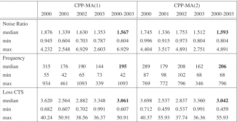
Table 1: CPP-MA Estimation Results for IBM Transaction Data 2000-2003
CPP-MA(1) CPP-MA(2)
2000 2001 2002 2003 2000-2003 2000 2001 2002 2003 2000-2003
Noise Ratio
median 1.876 1.339 1.630 1.353 1.567 1.745 1.336 1.753 1.512 1.593
min 0.945 0.604 0.703 0.787 0.604 0.996 0.915 0.973 0.804 0.804 max 4.232 2.548 6.929 2.603 6.929 4.404 3.517 4.891 2.751 4.891
Frequency
median 315 176 190 144 195 289 179 208 162 206
min 55 42 65 73 42 87 98 102 68 68
max 934 461 1093 339 1093 769 772 796 346 796
Loss CTS
median 3.620 2.564 2.882 3.348 3.061 3.698 2.537 2.837 3.360 3.042
min 0.682 0.607 0.702 0.991 0.607 0.712 0.459 0.537 0.991 0.459
max 40.24 50.91 38.56 36.37 50.91 40.37 55.93 37.74 36.36 55.93
Note. This table contains summary statistics for the daily estimates of the noise ratio (upper panel), optimal sampling frequency in
seconds (middle panel), and CTS loss in percentages (lower panel) for IBM transaction data over the period Jan 2000 until Aug 2003.
relatively complex, with the model parameters entering non-linearly, we undertake a simulation experiment to investigate the issue. Based on the CPP-MA(2) model and realistic parameter values (i.e.ρ= 0.6,λ(0,1)= 5000, σν/σε = 1.1, annualized return volatility of25%), we simulate a day worth of transaction data. We then estimate
the model parameters, integrated intensity process, and optimal sampling frequency (under BTS), compare these to their actual values and repeat the procedure several times. The right panel of Figure 2 reports a histogram of estimated optimal sampling frequency in the presence of measurement error based on 5000 simulation runs. The optimal sampling frequency based on the true parameters is 175 seconds. As expected, the estimated sampling frequencies do deviate from their true values but, quite surprisingly, the measurement error does not lead to a bias in the estimates. This finding contrasts sharply to the results reported in Bandi and Russell (2003) which illustrate that, within their proposed framework, measurement error renders the estimated optimal sampling frequency severely biased.
4.3 Empirical Results
FIGURE3: OPTIMALSAMPLINGFREQUENCY ANDINEFFICIENCY OFCTS
2000 2001 2002 2003
2 min 5 min 8 min 11 min 14 min
2000 2001 2002 2003
5 15 25 35 45
Note. The estimated daily optimal sampling frequency under BTS for IBM transaction data over the period Jan 2000 until Aug 2003 (left panel) with the associated CTS loss in percentage points (right panel).
optimal sampling frequency (left panel) and CTS loss (right) panel and Table 1 reports additional summary statistics.
Regarding the specification of the noise term, it is clear from Table 1 that the results are very similar for both models. The CPP-MA(2) model picks up a little more dependence which leads to a slightly lower optimal sampling frequency on average (206 seconds instead of 195 for the CPP-MA(1)) but the sample average of the daily estimates for ρ is still very close to zero (i.e. 0.0026). Hansen and Lunde (2004a) argue that the higher order non-iid type noise, such as the MA(2) specification, may be required for the modelling of the market microstructure in practice but that this is more important for the modelling of mid-quotes as opposed to transaction data. It therefore seems reasonable to conclude that the CPP-MA(1) is sufficiently flexible for the purpose and data set at hand. Although beyond the scope of the current paper, in future research we may explore extended versions of the CPP-MA model to investigate the importance of including higher order dependence, leverage effects, and non-Gaussian innovations.
FIGURE4: DETERMINANTS OF THE OPTIMALSAMPLINGFREQUENCY
2K 5K 8K 11K 14K
2 min 5 min 8 min 11 min 14 min
1.0 2.0 3.0 4.0 5.0
2 min 5 min 8 min 11 min 14 min
Note. Scatterplot of the estimated optimal sampling frequency under BTS versus the number of transactions (left panel) and noise ratio (right panel). The data is IBM transaction data over the period Jan 2000 until Aug 2003.
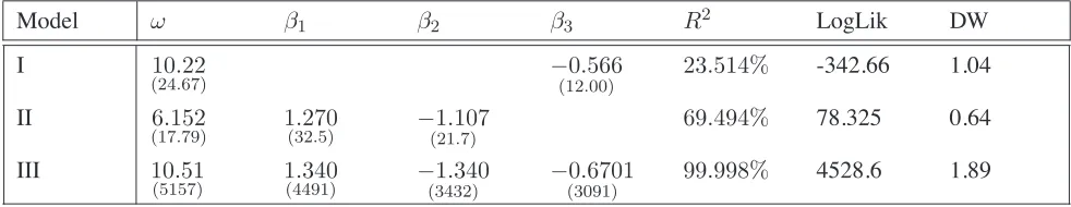
done at a fixed frequency for the entire sample, it is not a surprising results because market activity, market microstructure, and the statistical properties of returns, are known to change over time. To explore this point a little further, Figure 4 reports a scatter plot of the optimal sampling frequency in minutes on the vertical axis against the number of transactions (left panel) and noise ratio (right panel). While one would be tempted to argue that the price process can be sampled at higher frequencies on active trading days, this relation appears weak. On the other hand, variation in the optimal sampling frequency seems to be much more closely related to changes in the noise ratio. Another way to illustrate this issue is by means of the following linear regression:
log ˆFt=ω+β1log ˆσν,t+β2log ˆσε,t+β3log ˆλ(t,t+1)+.t (3)
whereFˆtdenotes the estimated day-toptimal sampling frequency based on the CPP-MA(1) model andλˆ(t,t+1)
Table 2: Optimal Sampling Frequency Regression for IBM Transaction Data 2000-2003
Model ω β1 β2 β3 R2 LogLik DW
I 10.22
(24.67) −(120..56600) 23.514% -342.66 1.04
II 6.152
(17.79) 1(32.270.5) −(211.107.7) 69.494% 78.325 0.64
III 10.51
(5157) 1(4491).340 −(3432)1.340 −(3091)0.6701 99.998% 4528.6 1.89
Note. Regression results forlog ˆFt = ω+β1log ˆσν,t+β2log ˆσε,t+β3log ˆλ(t,t+1) +%t whereF denotes the day−testimated
optimal sampling frequency under BTS based on the restricted CPP-MA(1) model. HAC consistent t-statistics are in parenthesis below
the estimated coefficient. The column “DW” reports the Durbin Watson statistic. April 18, 2002 is taken out to remove an outlier in the
optimal sampling frequency of 1093 seconds.
We are now left with the central question whether BTS does indeed lead to a lower MSE of realized variance. As shown above, the key to BTS superiority is the diurnal pattern of trade activity. Using the non-parametric techniques mentioned above, we estimate the trading intensity process for each day in the sample and then use the CPP-MA model to compute the daily difference in MSE under CTS relative to BTS at the optimal sampling frequency under BTS (whether to evaluate the MSE at the optimal sampling frequency under BTS or CTS here does not have a material impact on the results since both lie closely together in most cases). The results reported in Table 1 and the right panel of Figure 3 show that BTS did achieve a lower MSE than CTS on every single day in the sample. Although the average increase in MSE under CTS is a modest3%, the most important results is that BTS never does worse. A closer look at the instances when the CTS loss exceeded15%indicates that the gains of using the BTS scheme are particularly large on days with highly irregular trading patterns, early market closures, or sudden moves in market activity. The left panel of Figure 5 plots the trading intensity estimates for three of such days. For instance, on June 7, 2000 IBM trading activity surged due to a favorable analyst report. On that day the Dow Jones Business News headlined “Wall Street Closes Higher, Paced By IBM Rebound On Goldman Sachs Comments” and reported that “A late-day rally in IBM shares helped push stocks higher Wednesday. . . International Business Machines (IBM) jumped 8 3/8 to 120 3/4 after Goldman Sachs analyst Laura Conigliaro told CNBC that the computer maker should see revenue improvements in the second half of the year” (source: Factiva). The reason for the trading pattern on August 21, 2001 is unclear while on July 5, 2002 the market closed at 13.00. Despite the unusual market activity, the estimated CPP-MA(2) parameters for these days are very much in line with those on other days suggesting that this cannot explain the gains associated with BTS (i.e. June 7, 2000:ρ= 0.0308,σν/σε = 1.8060,λ(0,1) = 6274, optimal sampling frequency232seconds,
CTS loss of35.9%, annualized daily return volatility21.8%. August 21, 2001: ρ =−0.0096,σν/σε = 1.3404,
λ(0,1) = 4600, optimal sampling frequency192seconds, CTS loss of16.7%, annualized daily return volatility 14.2%. July 5, 2002:ρ =−0.1773,σν/σε = 1.2026,λ(0,1) = 4282, optimal sampling frequency178seconds,
FIGURE5: ESTIMATED TRADINGINTENSITY AND MSEONBTS FAVORABLEDAYS
10:00 11:00 12:00 13:00 14:00 15:00 16:00 0
2000 4000 6000 8000 10000 12000 14000 16000
June 7, 2000 (CTS loss of 35.9%) August 21, 2001 (CTS loss of 16.7%) July 5, 2002 (CTS loss of 29.5%)
1 min 2 min 3 min 4 min 5 min 6 min 7 min 8 min
2.00 3.00 4.00 5.00
MSE under BTS on June 7, 2000 MSE under CTS on June 7, 2000
Note. Left panel: non-parametric estimate of trading intensity. Right panel: MSE of realized variance under BTS and CTS for sampling frequencies between 1 and 8 minutes.
realized variance for June 7, 2000 based on the CPP-MA(2) model under CTS and BTS for sampling frequencies between 1 and 8 minutes. It can be seen that the reduction in MSE is substantial around the optimal sampling frequency. In fact, sampling at 8 minutes in BTS achieves the same MSE as sampling at 3 minutes under CTS!
5
Conclusions
A Appendix
Proof of Theorem 2.1. For a generalM A(q)-innovation structure define
rt(h) = h!−1
j=0
(εt−j+ηt−j) =
h−1
!
j=0
εt−j+ h−1
!
j=0
q
!
i=0
ρiνt−j−i = h!−1
j=0
εt−j+ h+q−1
!
j=0
min(j,q)
!
i=max(0,j−h+1)
ρiνt−j
forh >0andrt(0) = 0. From this it can be seen that the mean returnE[rt(h)] =h(µε+µvρ)whereρ=$qi=0ρiand the varianceV[rt(h)]≡Σq(h)is equal to:
Σq(h) = hσ2ε+hσν2 q
!
i=0
ρ2i + 2σ2ν
min(q,h)
!
j=1
q
!
i=j
(h−j)ρiρi−j
= h"σ2
ε+σ2νρ2 #
−2σ2
ν q ! j=1 q !
i=j
jρiρi−j forh≥q (4)
Moreover, the covariance betweenrt(h)andrt+k+m(k)forq > m≥0can then be worked out as: Ωq(h, k, m) ≡ Cov(rt(h), rt+k+m(k))
= Cov
h+q−1
!
j=0
min(j,q)
!
i=max(0,j−h+1)
ρiνt−j, k+q−1
!
j=0
min(j,q)
!
i=max(0,j−k+1)
ρiνt−(j−k−m)
= Cov
h+q−1
!
j=0
min(j,q)
!
i=max(0,j−h+1)
ρiνt−j, q−m−1
!
w=−k−m
min(w+k+m,q)
!
i=max(0,w+m+1)
ρiνt−w
= σν2
min(h+q−1,q−m−1)
!
b=0
min(b,q)
!
i=max(0,b−h+1)
ρi
min(b+k+m,q)
!
i=max(0,b+m+1)
ρi
(5)
andΩq(h, k, m) = 0forq≤m. Due to the joint normality ofrt(h)andrt+k+m(k), their characteristic function can be expressed as:
φq(h, k, m) ≡ E(exp{iξ1rt(h) +iξ2rt+k+m(k)}) = exp+i(µε+µvρ) (ξ1h+ξ2k)−
1 2
"
ξ12Σq(h) +ξ22Σq(k) + 2ξ1ξ2Ωq(h, k, m)#
,
(6)
Using the above, the joint characteristic function of returns,R(t1|τ1)andR(t2|τ2)for t2 ≥ t1+τ2, conditional on the
intensity process, can then be written as:
φRR(ξ1,ξ2|t1, t2,τ1,τ2, q) ≡ Eλ(exp{iξ1R(t1|τ1) +iξ2R(t2|τ2)})
= ∞ ! m=0 ∞ ! h=0 ∞ ! k=0
φq(h, k, m) λk
2
k!eλ2 λh
1
h!eλ1 λm
1,2
m!eλ1,2.
withλj,λi,j as defined in expression (2). This infinite triple summation over m, h,andkfrom zero to infinity can be simplified somewhat by decomposing it as follows:
∞ ! m=0 0 ! h=0 0 ! k=0 + ∞ ! m=0 ∞ !
h=q
∞
!
k=q +
∞
!
m=0
q−1
! h=1 ∞ ! k=1 + ∞ ! m=0 ∞ !
h=q q−1
! k=1 + ∞ ! m=0 ∞ !
h=q + ∞ ! m=0 ∞ !
k=q +
∞
!
m=0
q−1
! h=1 + ∞ ! m=0
q−1
!
where the double summations have the missing third argument set to zero.
φq(h, k, m) =
exp'iξ1h(µε+µvρ)−12ξ12Σq(h)( forh < q;k= 0 exp'ξ2
1c0+hc1( forh≥q;k= 0
exp'i(ξ1h+iξ2k) (µε+µvρ)−12ξ12Σq(h)−12ξ22Σq(k)−ξ1ξ2Ωq(h, k, m)( forh < q;k < q exp'iξ1h(µε+µvρ) +ξ22c0+kc2−12ξ12Σq(h)−ξ1ξ2Ωq(h, k, m)( forh < q;k≥q exp'iξ2k(µε+µvρ) +ξ21c0+hc1−12ξ22Σq(k)−ξ1ξ2Ωq(h, k, m)( forh≥q;k < q exp'"ξ2
1+ξ22
#
c0+hc1+kc2−ξ1ξ2Ωq(m)( forh≥q;k≥q where we use the notationΩq(m) =Ωq(h≥q, k≥q, m)and
c0=σ2ν q
!
j=1
q
!
i=j
jρiρi−j and cz=iξz(µε+µvρ)− 1 2ξz2
"
σε2+σ2νρ2 #
forz∈{1,2}. (7)
Some of the summations can now be simplified substantially, i.e. $∞m=0$qh−=11 ⇒ $hq−=11, $∞m=0$0h=0$0k=0 ⇒ e−λ1−λ2, and
∞
!
m=0 ∞
!
h=q
⇒ e−(λ1+λ2)
∞
!
h=q
φq(h,0,0) λh
1
h! = exp
'
ξ12c0−λ2+λ1(ec1−1)(
&
1−Γ(q,λ1ec1)
Γ(q)
) ∞ ! m=0 ∞ !
k=q
⇒ e−(λ1+λ2) ∞
!
k=q
φq(0, k,0) λk
2
k! = exp
' ξ2
2c0−λ1+λ2(ec2−1)(
&
1−Γ(q,λ2ec2)
Γ(q)
) ∞ ! m=0 ∞ !
h=q
∞
!
k=q
⇒ Ψq(ξ1,ξ2, q,Ωq) exp'"ξ12+ξ22
#
c0+λ1(ec1−1) +λ2(ec2−1)(
whereΓ(w) =.0∞uw−1e−udu(gamma function), andΓ(w, z) =.∞ z u
w−1e−udu(incomplete gamma function) and:
Ψq(ξ1,ξ2, q,Ωq) =
&
1−Γ(q,λ1ec1)
Γ(q)
) &
1−Γ(q,λ2ec2)
Γ(q)
) *
1−Γ(q,λ1,2)
Γ(q) +
q−1
!
m=0
e−ξ1ξ2Ωq(m) λ
m
1,2
m!eλ1,2
-(8)
Collecting all the yields the expression forφRR(ξ1,ξ2|t1, t2,τ1,τ2, q)given in Theorem 2.1.
Moment Expressions for the Restricted CPP-MA(2). Based on the characteristic function for the restricted CPP-MA(2), i.e.µν =µε= 0, andρ0= 1,ρ1=ρ−1,andρ2=−ρ, the following moment expressions can be derived:
Eλ /
R(ti|τi)2
0
= λiσ2ε+ 2σν2 "
1 +ρ2# "1−e−λi#
−2σν2ρλie−λi (9)
Eλ /
R(ti|τi)4
0
= 3λiσε4+ 3λ2iσε4+ 12λiσ2εσ2ν "
1−ρe−λi+ρ2#+ 12σ4 ν "
1 +ρ2#2"1−e−λi#
−12σ4νρλie−λi"2−ρ+ 2ρ2# (10)
Eλ /
R(ti|τi)2R(tj|τj)2
0
= λiλjσ4ε+ 2σε2σν2 "1 +
ρ2# "λ
i+λj−λje−λi−λie−λj#
−2λiλjρσ2εσν2 "
e−λi+e−λj#
−4σν4 "1 +
ρ2#2"e−λj
−e−λj−λi+e−λi
−1# −4e−λi−λjσ4
νρ "
1 +ρ2# "λieλj−λi+λjeλi−λj#+ 4e−λi−λjσν4ρ2λiλj
−2σν4e−λi−λi,j−λj 9"1 +
ρ2#2+λi,jρ2: "eλj+eλi−eλi+λj −1# +2σ4
νe−λi−λi,j−λj "2
References
Andersen, P. K., Ø. Borgan, R. Gill, and N. Keiding, 1993, Statistical Models Based on Counting Processes. Springer-Verlag, New York.
Andersen, T. G., T. Bollerslev, F. X. Diebold, and P. Labys, 2000, “Great Realizations,”Risk, pp. 105–108.
, 2003, “Modeling and Forecasting Realized Volatility,”Econometrica, 71 (2), 579–625.
An´e, T., and H. Geman, 2000, “Order Flow, Transaction Clock, and Normality of Asset Returns,”Journal of Finance, 55(5), 2259–2284.
Bandi, F. M., and J. R. Russell, 2003, “Microstructure Noise, Realized Volatility, and Optimal Sampling,” manuscript GSB, The University of Chicago.
Barndorff-Nielsen, O. E., and N. Shephard, 2004a,Continuous Time Approach to Financial Volatility. Cambridge University Press, forthcoming.
Barndorff-Nielsen, O. E., and N. Shephard, 2004b, “Econometric Analysis of Realised Covariation: High Fre-quency Based Covariance, Regression and Correlation in Financial Economics,”forthcoming Econometrica, 72.
Bowsher, C. G., 2002, “Modelling Security Market Events in Continuous Time: Intensity-Based, Multivariate Point Process Models,” Manuscript Nuffield College, University of Oxford.
Carr, P., H. Geman, D. B. Madan, and M. Yor, 2002, “The Fine Structure of Asset Returns: An Empirical Investigation,”Journal of Business, 75 (2), 305–332.
Carr, P., and L. Wu, 2003, “Time-Changed L´evy Processes and Option Pricing,” forthcomingJournal of Financial Economics.
Corsi, F., G. Zumbach, U. A. M¨uller, and M. Dacorogna, 2001, “Consistent Precision Volatility from High-Frequency Data,” Olsen Group Working Paper.
Cowling, A., P. Hall, and M. J. Phillips, 1996, “Bootstrap Confidence Regions for the Intensity of a Poisson Point Process,”JASA, 91 (436), 1516–1524.
Cox, J. C., and S. A. Ross, 1976, “The Valuation of Options for Alternative Stochastic Processes,”Journal of Financial Economics, 3 (1/2), 145–166.
Geman, H., D. B. Madan, and M. Yor, 2001, “Time Changes for Levy Processes,”Mathematical Finance, 11 (1), 79–96.
Hansen, P. R., and A. Lunde, 2004a, “An Unbiased Measure of Realized Variance,” manuscript Department of Economics, Brown University.
, 2004b, “Realized Variance and IID Market Microstructure Noise,” manuscript Brown University.
Karlin, S., and H. M. Taylor, 1981,A Second Course in Stochastic Processes. Academic Press, New York.
Maheu, J. M., and T. H. McCurdy, 2003, “Modeling Foreign Exchange Rates with Jumps,” manuscript University of Toronto.
, 2004, “News Arrival, Jump Dynamics and Volatility Components for Individual Stock Returns,”Journal of Finance, 59 (2).
Meddahi, N., 2002, “A Theorical Comparison Between Integrated and Realized Volatility,”Journal of Applied Econometrics, 17, 479–508.
M¨urmann, A., 2001, “Pricing Catastrophe Insurance Derivatives,” Manuscript Insurance and Risk Management Department, The Wharton School.
Press, S. J., 1967, “A Compound Events Model for Security Prices,”Journal of Business, 40(3), 317–335.
, 1968, “A Modified Compound Poisson Process with Normal Compounding,”Journal of the American Statistical Association, 63, 607–613.
Rogers, L., and O. Zane, 1998, “Designing and Estimating Models of High-Frequency Data,” Manuscript Uni-versity of Bath.
Rydberg, T. H., and N. Shephard, 2003, “Dynamics of Trade-by-Trade Price Movements: Decomposition and Models,”Journal of Financial Econometrics, 1 (1), 2–25.
!
!"#$%&'()*)+#,(,+#%+,(
(
List of other working papers:
2004
1. Xiaohong Chen, Yanqin Fan and Andrew Patton, Simple Tests for Models of Dependence Between Multiple Financial Time Series, with Applications to U.S. Equity Returns and Exchange Rates, WP04-19
2. Valentina Corradi and Walter Distaso, Testing for One-Factor Models versus Stochastic Volatility Models, WP04-18
3. Valentina Corradi and Walter Distaso, Estimating and Testing Sochastic Volatility Models using Realized Measures, WP04-17
4. Valentina Corradi and Norman Swanson, Predictive Density Accuracy Tests, WP04-16 5. Roel Oomen, Properties of Bias Corrected Realized Variance Under Alternative Sampling
Schemes, WP04-15
6. Roel Oomen, Properties of Realized Variance for a Pure Jump Process: Calendar Time Sampling versus Business Time Sampling, WP04-14
7. Richard Clarida, Lucio Sarno, Mark Taylor and Giorgio Valente, The Role of Asymmetries and Regime Shifts in the Term Structure of Interest Rates, WP04-13
8. Lucio Sarno, Daniel Thornton and Giorgio Valente, Federal Funds Rate Prediction, WP04-12 9. Lucio Sarno and Giorgio Valente, Modeling and Forecasting Stock Returns: Exploiting the
Futures Market, Regime Shifts and International Spillovers, WP04-11
10.Lucio Sarno and Giorgio Valente, Empirical Exchange Rate Models and Currency Risk: Some Evidence from Density Forecasts, WP04-10
11.Ilias Tsiakas, Periodic Stochastic Volatility and Fat Tails, WP04-09
12.Ilias Tsiakas, Is Seasonal Heteroscedasticity Real? An International Perspective, WP04-08 13.Damin Challet, Andrea De Martino, Matteo Marsili and Isaac Castillo, Minority games with
finite score memory, WP04-07
14.Basel Awartani, Valentina Corradi and Walter Distaso, Testing and Modelling Market Microstructure Effects with an Application to the Dow Jones Industrial Average, WP04-06 15.Andrew Patton and Allan Timmermann, Properties of Optimal Forecasts under Asymmetric
Loss and Nonlinearity, WP04-05
16.Andrew Patton, Modelling Asymmetric Exchange Rate Dependence, WP04-04
17.Alessio Sancetta, Decoupling and Convergence to Independence with Applications to Functional Limit Theorems, WP04-03
18.Alessio Sancetta, Copula Based Monte Carlo Integration in Financial Problems, WP04-02 19.Abhay Abhayankar, Lucio Sarno and Giorgio Valente, Exchange Rates and Fundamentals:
Evidence on the Economic Value of Predictability, WP04-01
2002
1. Paolo Zaffaroni, Gaussian inference on Certain Long-Range Dependent Volatility Models, WP02-12
2. Paolo Zaffaroni, Aggregation and Memory of Models of Changing Volatility, WP02-11
3. Jerry Coakley, Ana-Maria Fuertes and Andrew Wood, Reinterpreting the Real Exchange Rate - Yield Diffential Nexus, WP02-10
4. Gordon Gemmill and Dylan Thomas , Noise Training, Costly Arbitrage and Asset Prices: evidence from closed-end funds, WP02-09
5. Gordon Gemmill, Testing Merton's Model for Credit Spreads on Zero-Coupon Bonds, WP02-08
6. George Christodoulakis and Steve Satchell, On th Evolution of Global Style Factors in the MSCI Universe of Assets, WP02-07