University of Warwick institutional repository
This paper is made available online in accordance with publisher policies. Please scroll down to view the document itself. Please refer to the repository record for this item and our policy information available from the repository home page for further information.
To see the final version of this paper please visit the publisher’s website. Access to the published version may require a subscription.
Authors: D. J. GREENWOOD, K. ZHANG, H. W. HILTON and A. J. THOMPSON
Article title: Opportunities for improving irrigation efficiency with quantitative models, soil water sensors and wireless technology
Year of publication:
2009
Link to published version:
http://dx.doi.org/10.1017/S0021859609990487
Publisher statement:
Agricsci 29 10 08-09 1
Opportunities for improving of irrigation efficiency with quantitative models, soil 2
water sensors and wireless technology are reviewed 3
By 4
5
Short title: Irrigation with sensors and wireless technology 6
7
SUMMARY 1
2
Increasingly serious shortages of water make it imperative to improve the efficiency of 3
irrigation in agriculture, horticulture and in the maintenance of urban landscapes. The 4
main aim of this review is to identify ways of meeting this objective. After reviewing 5
current irrigation practices, discussion is centred on the sensitivity of crops to water stress, 6
the finding that growth of many crops is unaffected by considerable lowering of soil 7
water content and on this basis the creation of improved means of irrigation scheduling. 8
Next, attention is focussed on irrigation problems associated with spatial variability in 9
soil water and the often slow infiltration of water into soil, especially the subsoil. As 10
monitoring of soil water is important for estimating irrigation requirements, the attributes 11
of the two main types of soil water sensors and their most appropriate uses are described. 12
Attention is also drawn to the contribution of wireless technology to the transmission of 13
sensor outputs. Rapid progress is being made in transmitting sensor data, obtained from 14
different depths down the soil profile across irrigated areas, to a PC that processes the 15
data and on this basis automatically commands irrigation equipment to deliver amounts 16
of water, according to need, across the field. To help interpret sensor outputs, and for 17
many other reasons, principles of water processes in the soil-plant system are 18
incorporated into simulation models that are calibrated and tested in field experiments. 19
Finally it is emphasised that the relative importance of the factors discussed in this review 20
INTRODUCTION 1
2
Water shortage severely depresses yields in many parts of the world. Increasing 3
populations and diminishing supplies of geological water exacerbate the problem. Indeed, 4
FAO (2008) considers that by 2025, 800 million people could be living under conditions 5
of absolute water scarcity. The scale of these problems is illustrated by the fact that world 6
agriculture wastes 1,500 trillion litres of water, 0.6 of the 2,500 trillion litres of water it 7
uses each year- which is 0.7 of the world’s accessible water (Clay 2004). In southern 8
Europe, irrigation accounts for over 0.6 of the water use in most countries (European 9
Commission 2000). The problems are enormous and require immediate remedies. 10
The comprehensive monograph (Stewart & Nielsen 1990) gives an excellent 11
account of the various factors influencing irrigation and how to improve irrigation 12
efficiency of many crops. Recent attention has been given to improved cultural practices 13
including subsurface irrigation (Banedjschafie et al. 2008), and partial root zone drying 14
irrigation (i.e. irrigating one side of a row crop whilst leaving the other side dry and then 15
at the next irrigation irrigating the dry side and leaving the previously irrigated side dry) 16
(Saeed et al. 2008). Considerable effort has also been devoted to developing drought 17
resistant cultivars by conventional and GM techniques (e.g. Farooq et al. 2009), and in 18
the long-term this could result in improved water use efficiency. Yet there is still 19
considerable uncertainty about how to adjust timing and rates of irrigation in different 20
cropping systems. Practical advances in predicting irrigation requirements that are of 21
wide applicability are needed. They could be applied immediately over wide could be of 22
Recently there have been substantial improvements in knowledge about the 1
tolerance of crops to water stress and the ability of soils to supply water, which has led to 2
the application of deficit irrigation (i.e. keeping the soil below field capacity during most 3
of the growing season). Further, advances have been made in understanding the soil-4
water-plant economy, by the integration of this knowledge into simulation models, by the 5
improvement sensor techniques for monitoring soil and plant water and by the 6
introduction of wireless technology that facilitates the transmission of sensor data so that 7
it can be used to control irrigation and also technology that permits control of remote 8
equipment. Although there have been many recent reviews on various aspects of 9
irrigation (e.g. Debaeke & Aboudrare 2004; Bastiannssen et al. 2007; Costa et al. 2007; 10
Fereres & Soriano 2007; Steduto et al. 2007), none bring together the forgoing diverse 11
aspects of sensor driven irrigation. The objective of the present review is to do so, to 12
identify opportunities for improvement, and especially to highlight possible practical 13
applications. 14
15
CURRENT IRRIGATION SCHEDULING 16
17
Irrigation practice is often dominated by the availability and costs of water. If water is 18
readily available and cheap, its use is often profligate with consequent environmental 19
damage from leaching and soil compaction. In most of the world, however, there is a 20
shortage of water but supply is often outside the control of the farmer, and the farmer 21
usually accepts irrigation water whenever it is available, often when the crop does not 22
assessment but are based on experience on what seems to have given good results in the 1
past. Nevertheless, science-based methods of assessing irrigation needs have had an 2
impact on practice. An early and most important contribution was the introduction of a 3
formula (Penman 1948), derived from considerations of energy and aerodynamics, for 4
calculating evaporative loss from well-watered turf. The formula has been modified to 5
the widely used Penman-Monteith equation (Monteith 1973; McNaughton & Jarvis 1984) 6
but the main principles remain and evapotranspiration calculated in this way for turf is 7
usually referred to as a reference evapotranspiration and is designated by ET (Hatfield 8
1990); the meteorological inputs to the model are measured routinely in most 9
meteorological stations. Pan evaporation (evaporation from a large pan of water) usually 10
designated as Eo is similar to that for well-watered turf and is also measured routinely 11
(Hatfield 1990). However, the percentage crop cover and the “surface roughness” vary 12
with crop species and development stage and are generally different from those of turf. 13
To correct for these differences, ET is multiplied by a crop specific coefficient Kc, the 14
values of which for different crops during their growth have been tabulated (Allen et al. 15
1998; Savaa & Frenken 2002). So if the aim of irrigation is to add sufficient water to 16
compensate for that lost by evapotranspiration then this can be achieved approximately 17
by adding an amount of water equal to that lost by the calculated evapotranspiration 18
(Kc×ET) less rainfall. A weakness of using this approach for estimating water loss over 19
substantial periods is that errors are cumulative and so added irrigation water can become 20
out of step with requirement (Jones 2004). These methods have been used for estimating 21
irrigation requirement by both full irrigation and deficit irrigation practices. In full 22
a practice that results in excessive waste of water from drainage and from evaporation 1
from the soil surface. In deficit irrigation less water is applied than is needed to meet total 2
losses from evapotranspiration (Costa et al. 2007; Fereres & Soriano 2007). Soil 3
moisture deficit is important and can be defined as the volume of water needed to bring 4
the soil to field capacity (i.e. the minimum water content at which free drainage can 5
occur). The extent to which the soil moisture deficit can be allowed to fall without 6
reducing crop growth varies depending on the crop species and its stage of development 7
and on the environmental conditions: topics which are discussed in detail in this review. 8
Increased use of deficit irrigation promises to bring about considerable increases in water 9
use efficiency. 10
Irrigation scheduling using plant-based methods has been comprehensively 11
reviewed by Jones (2004). Several procedures for measuring plant water stress have been 12
devised but they generally require a good deal of expertise to operate and, in any event, 13
they do not indicate the water requirement. The most promising approach is thermal 14
imaging. It is based on measuring the drop in temperature resulting from the evaporation 15
of water. As loss of water from stomata is greater when they are open than when they are 16
closed, temperatures are lower. The temperature difference of course also depends on the 17
evaporative conditions in the surrounding atmosphere. Thus the techniques have been a 18
useful tool for irrigation scheduling in arid regions but less so in humid regions (Jones 19
2004). 20
On the other hand, irrigation scheduling-based on soil water has been widely 21
reported. The distributions of water down soil profiles have long been measured 22
inexpensive, convenient to operate and require little labour are being developed and are 1
increasingly used commercially. Some of them are described later in this review. Soil 2
water has also been monitored remotely by microwave radar techniques (Ragab 1995; 3
Clark et al. 2005: Jadoon et al. 2008; Lambot et al. 2008) generally for research and 4
specialized purposes. 5
6
PLANT AND SOIL PROCESSES AFFECTING IRRIGATION REQUIREMENTS 7
8
Opportunities for reducing the wastage of irrigation water include: 9
(1) reducing loss of water through evaporation from the soil surface; 10
(2) reducing leaching below the depth of rooting; 11
(3) allowing crops to exploit the water stored within the soil profile to the full depth 12
of rooting; in many parts of the world, winter rain or monsoons bring the soil to 13
field capacity and it is essential to make full use of this stored water; 14
(4) reducing the accumulation of salts within the soil profile that arise from excessive 15
irrigation. 16
All four objectives can be met, at least partially, by reducing the total application of 17
irrigation water. For example, if the frequency of irrigation is kept to a minimum then the 18
surface soil will dry out and less water will be lost by evaporation from the soil surface. 19
Plant factors influencing irrigation need 20
Static maximum allowable soil moisture deficits 21
The key to minimizing irrigation without inhibition of growth is the often repeated 22
rate (Bailey 1990; Hills et al. 1990; Krieg & Lascano 1990; Musick & Porter 1990; Bacci 1
et al. 2003; Panda et al. 2003). Much effort has therefore been devoted to quantifying 2
this phenomenon (Denmeade & Shaw 1962; Ritchie 1973; Meyer & Green 1980; 3
Rosenthal et al. 1987; Muchow & Sinclair 1991; Sadras et al. 1993; Sadras & Milroy 4
1996; Thompson et al. 2007). A summary of this work is given in the FAO irrigation 5
manual (Allen et al. 1998; Savva & Frenken 2002). It considers that water stress does not 6
inhibit growth unless it also inhibits evapotranspiration. It is based on the assumption 7
that crop evapotranspiration remains constant with a decrease in available water until a 8
value is reached after which evapotranspiration declines linearly with a further decrease 9
in available water until the wilting point is reached when evapotranspiration ceases. It 10
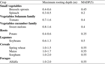
summarizes existing knowledge in terms of a maximum allowable soil moisture deficit 11
expressed as a proportion of the available water to the depth of rooting (MADP). The 12
concept is illustrated by the diagram given in Fig. 1. 13
14
MADP = RAW/TAW (1)
15
16
where TAW is the total available water in the root zone, i.e. between field capacity and 17
the permanent wilting point. RAW, the readily plant available water, is the proportion of 18
TAW that can be removed before transpiration and growth rate start to decline. MADP 19
depends on plant species and the evaporative conditions. Values of MADP standardized 20
to a value of ET = 5 mm d-1 (the reference evapotranspiration) and referred to as MADP 21
(5), have been provided by Allen et al. (1998) for 92 different crops. Examples are given 22
of MADP to be adjusted for differences in ET, over the range 0.1 ≤ MADP(ET) ≤ 0.8. It 1
is 2
3
MADP(ET) = MADP(5) + 0.04(5-ET) (2)
4
5
MADP(ET) is the value of MADP for a given value of ET in mm d-1. Perhaps the 6
equation should be treated with some caution as there has been a long standing 7
controversy about the dependence of MADP on ET (e.g. Denmeade & Shaw 1962; 8
Ritchie 1973). These estimates of the MADP’s for different crops can only be 9
approximate as Eqns (1) and (2) are assumed to hold for all soils and environments. 10
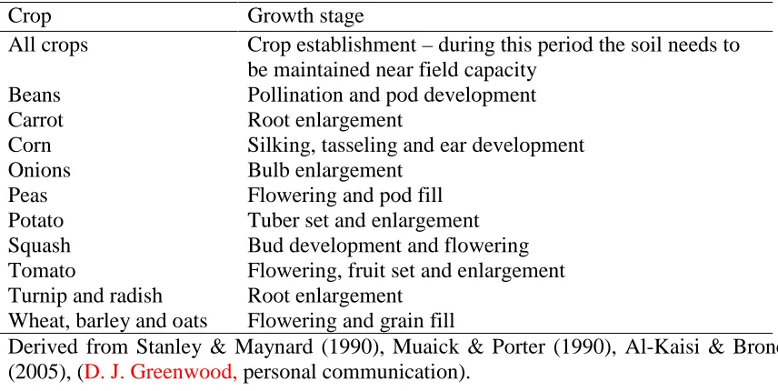
Dynamic maximum allowable soil moisture deficits 11
Implicit in the FAO tables of MADP(5) (Allen et al. 1998) is that MADP(5) for each 12
species is considered to remain constant throughout growth, even though it has long been 13
established that the sensitivity of crop growth to water stress varies during the growing 14
season (Salter & Goode 1975). Recent work summarizing the more sensitive stages of 15
growth over a range of crops is illustrated in Table 2, and emphasizes that crops are 16
particularly sensitive to water stress at flowering and seed development. Also, the method 17
does not take account of the short-term changes in evaporative demand, plant water stress 18
and growth rate during the growth period. The reason for the omission of these aspects 19
from the FAO tables could be that the bulk of experiments on which they are based only 20
reported the net effects of the soil average water deficit during growth on crop yields and 21
provided little information on the short-term changes during the growing period. 22
applying irrigation whenever the soil moisture deficit fell to each of different extents 1
during growth. It enabled the minimum soil moisture deficit for maximum final yield to 2
be estimated, which together with the depth of rooting gave the MADP. 3
One possible way of obtaining better information about changes during growth of 4
allowable soil water deficits is to base it on the finding that, although growth increases 5
almost asymptotically with increase in transpiration, growth and transpiration over a wide 6
range of conditions are almost proportional to one another with a gradient that depends 7
on evaporative conditions (Guitjens 1990; Steduto et al. 2007). Thus in some lysimeter 8
experiments, once there is complete crop cover of the soil the rate of loss of water is 9
assumed to be proportional to growth rate. Also from the daily loss of water the average 10
soil water content can be estimated. Non-destructive measurements of transpiration and 11
soil water content as in some lysimeter experiments can provide a good indication of 12
changes in the sensitivity of growth to soil water stress over much of the growing period. 13
Another approach to the problem is to relate surrogate measures of plant growth 14
rate, such as the rate of leaf expansion, to plant available soil water (PAW) (Sadras & 15
Milroy 1996). Essentially plant measurements are made at intervals over a period during 16
which the soil water content to the depth of soil containing most roots declines. The rate 17
of the surrogate process measured on the stressed plant relative to that on the unstressed 18
plant is considered to be unaffected by fall in water content until a threshold value is 19
reached when the rate starts to fall. This threshold value and the corresponding apparent 20
maximum allowable deficit expressed as a fraction of the total available water are 21
determined. They are analogous to MADP and they are broadly consistent (Sadras & 22
The rooting depth problem 1
All the above methods suffer from the drawback that the amount of crop available 2
water is critically dependent on the depth of rooting which is often very difficult to 3
estimate. A major problem in generalizing the results at one site to others is that rooting 4
depths are very sensitive to soil conditions (Taylor & Gardner 1963; Stalham et al. 2007) 5
as is illustrated by Fig. 2 which shows that root penetration can vary by four fold over the 6
normal range of soil resistances induced by compaction and by reduced soil water content. 7
Field experiments and surveys on 602 UK commercial fields of potatoes demonstrated 8
that compaction resulted in shallower rooting than is desirable for efficient use of water 9
and nutrients (Stalham et al. 2007). Practically useful models are needed to predict the 10
effects of soil conditions throughout growth. A possible way forward is suggested by the 11
finding that penetrometer measurements can give a good measure of the effect of soil 12
conditions on root growth at a point in time (Clark et al. 2005). It may be possible to 13
develop models for the dependence of penetrometer readings and thus root penetration on 14
soil texture, soil organic matter content and soil water content and thus provide a means 15
of estimating the effects of changes in soil conditions on root penetration over long 16
periods.. 17
A new procedure for measuring the maximum allowable deficits without any 18
explicit requirement of rooting depth was introduced by Thompson et al. 2007 for crops 19
in a 40 cm deep soil. Measurements are made of volumetric water content to this depth 20
every 30 minutes. The loss of water is partitioned into drainage and transpiration losses 21
by considering that only drainage loss occurred at night. It is considered that when 22
the MADP can be calculated from the corresponding soil water content The idea that the 1
net changes in soil water content from drainage (and also from evaporation) can be 2
assessed from measurements during the night might have wider applications. They may 3
be relevant to estimating the depth of rooting from sensor measurements of soil water 4
down the soil profile. The depth of rooting is sometimes taken as the maximum depth at 5
which soil water content declines according to measurements at a given time of day. This 6
could be due to a combination of transpiration, drainage, and other soil processes 7
affecting water movement. Ideally what is required is the depth from which transpiration 8
removes water. By taking account of changes in soil water during the night, it should be 9
possible to separate the changes due to soil processes from those due to transpiration and 10
thus obtain a more reliable measure of rooting depth. 11
12
Soil factors affecting irrigation need 13
Soil variability across the field 14
A major limitation to irrigation efficiency of many arable crops can be differences in 15
irrigation requirement across fields which are associated with variations in soil hydraulic 16
properties (Ahuja & Nielson 1990). Ideally measurements of hydraulic properties over 17
the irrigated area need to be made and interpreted with kriging techniques to produce 18
contour diagrams of the variation in hydraulic conductivity. These measurements are, 19
however, too costly and there is a need for short-cut cheaper procedures. Soil surveys 20
provide data on soil properties to depth which is important as deep rooted crops can 21
extract much water from the subsoil. Information gained in this way, or even better by 22
content can be used to infer soil hydraulic properties by means of pedo-transfer functions 1
(PTFs). Several PTFs have been proposed including those based on the HYPRES 2
database (Lilly et al. 1998), which covers different European soils (Wösten et al. 1999). 3
Thermal imaging (Jones 2004), airborne radiometric surveys (Rawlins et al. 2009) and 4
grain yields which are often measured routinely across fields by farmers, can also provide 5
useful information. 6
Water use efficiency could be improved by monitoring soil water contents down 7
the soil profile, at different locations, and adjusting irrigation practice accordingly. In 8
practice it seems too time consuming and costly to do this manually, with a neutron probe 9
or similar device, but as will be shown later it should be possible to do so, relatively 10
cheaply, using soil water sensors combined with wireless technology. 11
Distribution of irrigation water 12
Another cause of variation is that most irrigation equipment does not distribute water 13
uniformly (Losada et al. 1990) and in consequence application of the amount of water 14
required to meet the average soil moisture deficit results in too little water being applied 15
at some locations and too much in others with consequent leaching and waste of water. 16
Poor water use efficiency can also be caused by irrigation failing to intercept plant roots. 17
While this is not a problem with drip irrigation, it is a problem especially with boom 18
irrigation of wide spaced crops and of pot and container plants because a large proportion 19
of the irrigation misses the plants. 20
Infiltration of water into soil 21
Effective irrigation requires that water penetrates soil rapidly. It is particularly important 22
applying heavy applications of water albeit occasionally. It is thus essential that the soil 1
permits rapid infiltration of water over long periods as occurs in well structured soils. 2
Rates of infiltration into some soils, however, fall very sharply to a low value shortly 3
after the start of irrigation (Kruse et al. 1990). Slow rates can usually be attributed to 4
compaction and small water filled pores through which water can pass only slowly but it 5
can result from the soil surfaces being water repellant (Bryant et al. 2007). Water 6
repellency occurs worldwide (Dekker et al. 2005) probably because of the deposition of 7
hydrophobic organic materials on soil surfaces (Debano 1971; Nannipieri & Badalucco 8
2003). Also some bacteria can produce extracellular polymeric substances in soil that can 9
bring about a four fold reduction in hydraulic conductivity (Or 2007). 10
Irrigation and rain can lead to surface sealing in some soils (e.g. Silva 2007); the 11
process results from disintegration of soil crumbs, swelling of soil colloids and 12
entrapment of air (Payne 1988 p.315). It has long been recognized as a major problem 13
and it has been alleviated in soils by application of soil conditioners (Ben-Hur et al. 1989) 14
and by various soil management practices (Abrisqueta et al. 2007). Barriers to water 15
penetration can of course also occur within the body of the soil profile. Well known 16
examples are plough and iron pans (Avery 1990). But such restrictions can also occur for 17
less well understood reasons; thus when a limited volume of water is added to some soils 18
the water content is brought to a uniform water content to a given depth but there is a 19
sharp boundary between this wetted soil and the unwetted soil beneath it (Russell 1973, p 20
435). The sharp transition could result from the hysteresis of the soil moisture release 21
curve (Warrick 1990) where the relation between water content and water potential 22
moving from the wet soil to the dry soil beneath consists of desorped water moving to 1
sorped water. Owing to hysteresis the water content on the wet side could be much 2
greater than on the dry side but they both have the same water potential and thus there is 3
no transfer of water. Inducing some soils to accept substantial volumes of water can be 4
difficult but a procedure which consisted of drilling holes to a depth of 60 cm, filling 5
them with sand and then irrigating (Abu-Awwad 1998) has resulted in deep penetration 6
of water and good crops on an impermeable soil. 7
Models for infiltration are of two types. One consists of empirical relationships 8
between various measurements for a particular area. The other is derived mechanistically 9
from the Richards’ equation and some of these models take account of hysteresis (Hanks 10
& Cardon 2003). As far as we are aware, however, none take account of soil water 11
repellency. 12
13
SENSORS 14
Required characteristics 15
Soil water sensors need to measure soil water content or the corresponding soil 16
water potential over the ranges that are found in practice. A recent survey of MADP(5) 17
on 22 different crop species gave 72 values that ranged from 0.05 to 0.81 with 26 values 18
being greater than 0.5. The majority of MADP(5) were therefore less than 0.5 (D. J. 19
Greenwood, personal communication). A proportion of 0.5 of the maximum available 20
water corresponds to a water potential of approximately -20 kPa for a loamy sand soil 21
and -200 kPa for a clay soil. A different survey gives 33 values of the soil water 22
were less than -200 kPa (D. J. Greenwood, personal communication). The results from 1
the two surveys are broadly consistent with one another and suggest that water potential 2
sensors over the range 0 to -200 kPa should cover most requirements. These values are, 3
however, averages, and water is unevenly distributed down the soil profile so the water 4
potential in a specific position, say at the uppermost sensor, could be much lower than -5
200 kPa. Variations between sensors of the same type in their responsiveness to soil 6
water should be small otherwise the cost of calibration could be considerable. Ideally 7
sensors should need no calibration by the user, and it is notable that according to 8
Decagon Devices (2009) one of their sensors meets this requirement. 9
There is no advantage of using sensors that measure water content over those that 10
measure water potential because the ability of a given soil to supply water to plant roots 11
is governed by both water potential and water content. Irrigation requirement is 12
dependent on soil water content at field capacity and the threshold value. So whichever 13
type of sensor is used the soil moisture release curve is required to calculate the missing 14
parameter and thus the irrigation requirement. 15
Available sensors 16
Numerous sensors for monitoring soil water are presently on the market; there are two 17
main types; those that measure soil water content and those that measure soil water 18
potential. The majority of the former actually measure the dielectric constant of soil, 19
which is largely determined by its water content. One type of dielectric sensor, frequency 20
domain reflectometer (FDR), also referred to as a capacitance sensor, adjusts the 21
frequency of an oscillating voltage until it identifies the strongest resonating frequency, 22
Another type of dielectric sensor uses the technology ‘time domain reflectometry’ (TDR) 1
to measure the dielectric constant, as the time taken for an electromagnetic pulse, 2
traveling down a rod to be reflected along its precise length. Both types of sensor, 3
although expensive, measure a wide range of bulk soil water contents. They can also 4
respond quickly to changes in soil water content (Campbell & Anderson 1998; Evett & 5
Parkin 2005; Nemali & Iersel 2006). However there is evidence that the performance of 6
some sensors may vary with the soil conditions; one commercially available capacitance 7
probe did not give reliable absolute measurements of soil water content although it 8
enabled relative changes in soil water content over time to be estimated (Mwale et al. 9
2005). Although they do not always give reliable measurements of soil water content, 10
dielectric sensors are generally chosen where there is a requirement to measure small but 11
rapid changes in soil water contents needed for precise control of water addition to soil. 12
For example, in container cropping where volumes of soil are small and it is essential to 13
maintain soil water contents close to a constant value, despite sudden variations in 14
evaporative conditions that in the absence of irrigation would cause rapid changes in soil 15
water content. 16
Moisture sensors that measure water potential are numerous. However, prominent 17
among sensors that have been used to measure water potential in field soils are granular 18
matrix sensors. Essentially, they consist of two concentric electrodes embedded in a 19
reference matrix material, which is surrounded by a synthetic membrane for protection 20
against deterioration (Chard 2005). When a sensor is put into moist soil, the matrix water 21
equilibrates with that in soil. Absorption of water increases the electrical conductivity of 22
are comparatively inexpensive, have a range of 0 to -240 kPa, can measure water 1
potentials in small volumes of soil, and have functioned satisfactorily in soil for 3.5 years 2
after installation (Qualls et al. 2001). They are, however, slow to respond to changes in 3
soil water content, especially in drier soils. Granular matrix sensors are usually chosen 4
when soil water changes are gradual, where many sensors are required to monitor soil 5
water to depth over considerable areas, and where satisfactory sensor performance over a 6
long period is required. 7
A novel and, probably more accurate sensor for measuring soil water potential 8
consists of porous material that equilibrates with the soil water and a dielectric device 9
that measures the water content of the porous material. A closed-form of hysteresis loop 10
is used to convert the measured water content of the porous material into water potential. 11
The use of two ceramic materials instead of one enables the sensor to measure matric soil 12
water potentials over the approximate range -10 kPa to -200 kPa. (Whalley et al. 2001; 13
Whalley et al. 2007; Whalley et al., in press). 14
Practical experience in the use of sensors 15
Much experience has been gained on the use of soil water sensors from which the 16
following practical advice on their use has emerged. 17
(a) Sensors must be calibrated for the given soil before use. Problems can arise, 18
however, because of failure to recognize that soil water potential sensors can only 19
operate over a limited range of water potentials and that equilibration times can be 20
considerable. Manufacturers of some types of sensors provide experimental 21
protocols for deriving calibration equations and others are published in the 22
addition to calibration, it is also important to check the specifications to ensure 1
that the sensor is suitable for the proposed application and soil. 2
(b) Protocols for embedding sensors in soil (Allen et al. 1998; Savva & Frenken 2002) 3
are especially important for small sensors as it is easy to damage the ceramics 4
(Bacci et al. 2003) which results in poor contact with the soil. Dielectric sensors 5
must be maintained in close contact with soil otherwise measurements can be 6
largely dominated by air gaps between sensor and soil. 7
(c) Failure to include a means of detecting sensor or electronic malfunction and an 8
associated routine for automatically cutting off the irrigation can result in 9
considerable waste of water (Qualls et al. 2001). 10
(d) The presence of roots around sensors can, if the sensors are small, result in their 11
outputs loosing sensitivity to changes in soil water, possibly because the sensors 12
become coated with material that is impermeable to water (Bacci et al. 2003). 13
14
IRRIGATION SCHEDULING BY SOIL WATER SENSORS 15
16
The use of these procedures varies enormously with the type of crop and the environment. 17
Sensor technology had been used at one extreme for crops grown for short periods, in 18
limited volumes of soil and under high evaporative conditions, and at the other extreme 19
for field crops grown over long periods in deep soils from which the roots extract water 20
up to 2 m from the surface. These differences result in variations in sensor costs and in 21
their performance. 22
Typical examples are container crops, lawns and urban landscapes as the rooting depths 1
are often no more than about 20 cm, often because they overlay a very compact soil layer, 2
or an extremely stony horizon that is a barrier to root penetration. The water contents in 3
such soils change very quickly and water needs to be added frequently so as to ensure 4
that the plant is never restricted by temporary water stress and yet ensure there is only 5
minimal drainage. Soil water sensors at only one depth are required for these cropping 6
systems. 7
Horticultural plants, such as ornamentals for the retail market are grown in 8
containers under evaporative conditions that are often high and vary during the day and 9
from day to day. Efficient irrigation practice has included taking readings at a specific 10
time of day and adjusting irrigation practice for the evaporative conditions (Klein 2004). 11
The amount of water that can be held in the rooting medium for container crops is small 12
so the water content can change quickly. What is required is a way of maintaining the soil 13
water at a constant value irrespective of changes in weather conditions, an objective that 14
has been achieved by Nemali & Iersel (2006). They devised a system in which a 15
controller uses dielectric substrate moisture sensors interfaced with a datalogger and 16
solenoid valves that supply irrigation. Measurements of substrate water were made every 17
20 minutes which enabled the substrate water content to be maintained within 2-3 % of 18
the target value over 40 days. The key to the success was the use of a very rapidly 19
responding dielectric sensor. 20
Sensor driven irrigation systems for urban landscapes in China and the USA are 21
described in a number of papers (e.g. Qualls et al. 2001; Guo et al. 2005). Scheduled 22
water loss from evaporative demand. However, in one system (Qualls et al. 2001) 1
granular matrix sensors (Watermark) were embedded in soil at different points within the 2
area and transmitted their readings by wire to an electronic module that either allows or 3
prevents a scheduled irrigation cycle depending on the soil moisture condition. The 4
system was adopted on 22 sites and the average area of each site was 2177 m2, resulting 5
an in an average saving of 27% of water and of 331 $US yr-1 per sensor. 6
Irrigation of lawns has, as for urban landscapes, been based on supplying 7
sufficient water to compensate for estimated evaporative demand. It can result in 8
excessive drainage losses. To prevent such losses, sensors that detect free water are 9
embedded in soil at a suitable depth, and when they indicate the presence of free water 10
they send a signal that cuts off the irrigation supply (Stirzaker & Hutchinson 2005). A 11
rather more sophisticated system has been reported, using a simulation model to estimate 12
water requirement together with a subsurface time domain sensor to monitor soil water 13
content (Blonquist et al. 2006). Its use resulted in 53% less irrigation than the currently 14
recommended fixed rate of 50 mm water per week and also resulted in no detectable 15
drainage below 30 cm from the surface. 16
Few papers in the literature are on sensor controlled irrigation of field crops that 17
penetrate to only a shallow depth. One such paper (Kang & Wan 2005) related the growth 18
and quality of radish (Raphanus sativus L.) to sensor measured water potentials at 20 cm 19
from the surface. It reported that although maintaining water potentials at each of 20
different values over the range -15 to -65 kPa had no affect on yield, they affected root 21
cracking which is an important quality attribute. A literature review of irrigation 22
indicated that good growth of a variety of crops required a water potential greater than -1
65 kPa (Boote & Ketring 1990; Stanley & Maynard 1990; Wright & Stark 1990; Munoz-2
Carpena et al. 2005; Wang et al. 2007). It is possible that at least some of these crops are 3
deep rooted. 4
As mentioned earlier, sub-surface drip irrigation (Banedjschaffe et al. 2008), can, 5
by minimizing evaporation from the soil surface, improve water use efficiency. It is 6
notable that water sensors at only 5 cm depth have been effectively used to control 7
decisions by irrigation from drip tapes installed 25-30 cm from the soil surface 8
(Noguerira et al. 2003). Sensors at shallow depths within the soil profile can therefore 9
provide useful information for irrigation scheduling. 10
Deep rooted agricultural crops 11
Limited support for the view that sensor determinations at about 25 cm depth may 12
provide a useful indication of irrigation need of some deeper rooted crops is provided by 13
Steiber & Shock (1995). These authors concluded that irrigation of potatoes could best be 14
determined by maintaining soil water potential above -59 kPa with sensors at a single 15
depth of between 0.1 and 0.2 m offset from the centre of the ridge. 16
Crops with roots that penetrate to a depth of 1 to 2 m can, if the soil conditions are 17
satisfactory, extract water to that depth. Many such soils are at near field capacity 18
immediately before planting, often as a result of winter rainfall or monsoon rains. 19
Considerable soil water deficits can occur on such soils without growth being inhibited. 20
Irrigating according to the distribution of soil water down the profile so as to make 21
maximum use of the stored water could therefore enable substantial saving of irrigation 22
periods which would reduce evaporation from it. For these reasons, some growers have 1
been using sensors to monitor soil water at different depths down the profile and using 2
the information obtained to schedule irrigation as described by free advice from extension 3
services (Thomson & Ross 1996; Werner 2002). 4
Estimation of when and how much irrigation is required for deep rooted crops can 5
be based on MADP using the information and sequence of decisions summarized in Fig.3. 6
Determinations of the rooting depth and volumetric water content to that depth require 7
further explanation. Thomson & Ross (1996) inferred the rooting depth from soil water 8
distribution measured by sensors. Other workers deduced the time course of the depth of 9
rooting from mean daily temperatures (Pedersen et al. 2009) or an algorithm that enables 10
the rooting depth to be calculated from plant dry weight (excluding fibrous roots), depth 11
of rooting at final harvest and an equation that defines the increase in plant dry weight 12
with time (e.g. Greenwood et al. 1977; Greenwood et al. 1982; Zhang et al. 2007). The 13
average volumetric water content to the depth of rooting can be calculated from the 14
measured soil water potentials down the profile and the soil water release curves. These 15
calculations can be aided by models that are subsequently described. 16
17
WIRELESS TECHNOLOGY 18
19
Wireless data acquisition and control systems (WDAC) will have an increasing impact on 20
many aspects of crop production. They enable data obtained from sensors or data loggers 21
to be received and facilitate remote control of a device through standard telephone lines, 22
data collection, variable rate technology and in disseminating information (Wang et al. 1
2006). Using WDAC systems to control irrigation should enable 2
(i) equipment to be remotely, and possibly automatically operated, for example 3
from control centre on the basis of the sensor data (Damas et al. 2001), 4
(ii) sensor readings at different depths and in different locations within a field to 5
be transmitted at predetermined times to a control centre where they are 6
processed, and possibly used to control equipment, 7
(iii) real time data to be made available over the Internet (Shulka et al. 2006) . 8
9
Much less work has been published on the use of WDAC systems for the control of 10
equipment than for the acquisition of data. Remote wireless controls of a central pivot 11
irrigation system (Pocknee et al. 2004) and of drip line irrigation (Coates et al. 2006) are 12
examples of the few publications of wireless control systems. By contrast, a literature 13
search (D.J Greenwood, personal communication) revealed 16 papers describing 14
successful wireless data acquisition systems (e.g. Bratton et al. 2000; Cao et al. 2005; 15
Kim et al. 2007; Vellidis et al. 2008). It seems that problems of installing effective 16
wireless acquisition systems have been largely solved but there are still technical 17
problems in wireless control of remote equipment. An encouraging development is that a 18
USDA group is studying wireless based irrigation control of self propelled linear-move 19
and centre-pivot irrigation equipment (Wang et al. 2006). 20
Recent advances for field crops include a wireless sensor means of scheduling 21
irrigation for field crops described by Vellidis et al. (2008). It also has the merit of being 22
field and a base station that consists of a receiver to accept wireless signals from the 1
nodes and a laptop to process the signals. At each node, sensors monitor soil water 2
potential at depths of 0.2, 0.4 and 0.6 m from the soil surface. They are connected by wire 3
to a specially-designed smart circuit board, mounted on top of a flexible rod, which at 4
predetermined times obtains readings from each of the sensors, activates a radio 5
frequency identification tag (RFID) and transmits the data to the base station; during the 6
remaining periods the node ‘sleeps’, does not use power, and over the entire growing 7
period only requires a single 9V lithium battery. The transmitter has a range of 0.8 km 8
provided there are no obstructions in the line of site to the base station. The procedure 9
was tested in a cotton field in which there were four different soil types. It appeared to 10
give excellent measurements of the distributions of soil water potential down the profiles 11
in each of them. In addition, outputs from the laptop have been linked to a variable rate 12
central pivot irrigation system so as to supply water at rates according to the needs of 13
individual areas within fields. Complete systems of sensors, wireless transmitters and 14
receivers are now available commercially (Decagon Devices 2009) and integrated 15
wireless communication and data logger systems are also on the market (Shukla et al. 16
2006). 17
Improvements in commercial wine production have been achieved by controlling 18
irrigation with high density multiple depth soil moisture sensors and transmitting the 19
outputs by wireless communication at 10 minute intervals to a central PC for processing 20
and storage on a database and estimating irrigation requirements. It was also transmitted 21
A major opportunity for advance in sensor controlled irrigation is provided by 1
recent research in wireless sensor networks which are impacting on many subjects. 2
Essentially it is concerned with the design of networks in which some of the nodes can 3
communicate with each other so that information can travel over short distances 4
(requiring little battery power) from node to node until it reaches the base station. This 5
enables low cost sensors to be distributed over a wide area and results in long battery 6
lives at the nodes and therefore little maintenance (Hart & Martinez 2006). 7
Wireless technology has recently been introduced into glasshouse 8
cropping to facilitate the retrieval of sensor information. Prior to this innovation, sensor 9
driven irrigation has involved extensive wiring that degrades under these conditions, 10
requires substantial maintenance and is quite impracticable in modern large glasshouse 11
systems. In consequence, current work is focused on devising combined wireless-12
transmitter-sensor modules that are distributed throughout the glasshouse and that 13
transmit to a computer controlled irrigation system (Cayanan et al. 2008). Such wireless-14
soil water sensor systems for glasshouses are now marketed commercially (Hoogendoorn 15
2008). 16
17
QUANTITATIVE MODELS 18
Simulation models for soil water and its effect on crop growth 19
Principles about water dynamics in the soil-crop system, such as those described above, 20
have been encapsulated into simulation models that calculate changes in soil water and 21
(Belmans et al. 1983), CROPWAT (Clarke 1998), IRSIS (Raes et al. 1988) and SWAP 1
(Kroes et al. 2008) . They aim to provide a widely applicable means of estimating water 2
distributions down the soil profile and their effects on plant growth. SWAP is one of the 3
most sophisticated models of its kind. The model simulates transport of water, solutes 4
and heat in the vadose zone interactively with the development of vegetation. The 5
governing equation for soil water flow is solved using an implicit finite difference 6
method. The model has been widely tested and has given promising results. However, 7
such a complex model requires many data inputs, which could cause difficulties for any 8
user who has not got an excellent knowledge of soil and plant sciences. Furthermore, the 9
adopted chosen numerical scheme is associated with instability. The most recent model, 10
AquaCrop, developed by FAO (Steduto et al. 2009; Raes et al. 2009a, b; Hsiao et al. 11
2009), simulates the effects of the aerial environment and soil water on plant processes. 12
The model updates for each day a range of variables. It calculates canopy cover, root 13
distribution, stomata opening, the roots ability to meet transpiration demand and 14
transpiration. Each of these variables depends to different extents on thermal time, 15
potential evapotranspiration and soil water stress which is calculated from the fraction of 16
available soil water to the depth of rooting. Plant biomass is calculated from transpiration 17
and is modified for atmospheric CO2 and soil fertility. Water evaporates from the soil 18
surface that is not covered by crop canopy. Water movement throughout the body of soil 19
is calculated by a cascade method using semi-empirical algorithms. The model has been 20
calibrated and tested against field experimental data for some crops with promising 21
results (e.g. Farahani et al. 2009; Hsiao et al. 2009). In the model, soil water is central to 22
appears to be questionable for some circumstances such as where there is a relatively 1
high groundwater table and upward capillary flow makes an important contribution 2
towards meeting evapotranspiration. Further, the model requires a large number of inputs 3
which are often difficult to obtain such as those associated with soil water movement. 4
Cascade methods, though easy to implement, are associated with unsatisfactory 5
simulations of capillary flow and poor predictions of daily soil water changes (Gandolfi 6
et al. 2006; Cannavo et al. 2008; Yang et al. 2009). If a way could be found of replacing 7
the cascade method in the AquaCrop model with ones based on the fundamental theory of 8
soil water movement then the resulting model might be more widely applicable than the 9
current version. 10
Application of classical theory of soil water movement 11
Application of this theory, besides improving existing models for water dynamics in the 12
soil-crop system, is also important for interpreting soil water sensor data. Although there 13
are many situations where soil water content increases with depth and the total soil 14
moisture deficit can be readily obtained from the integral of a fitted empirical equation 15
between sensor measured soil water content and depth, there are other situations where 16
the patterns are complex and the fitting procedure is unsatisfactory, especially when soil 17
sensors are few. Also it is always difficult, from soil sensor measurements, to distinguish 18
between evaporative and drainage losses and crop transpiration. 19
The key to solving these problems probably lies in applying classical theory of 20
soil water transport, despite complications associated with the dependence of the soil 21
water content is rising or falling (Warrick 1990). Classical theory is encapsulated in the 1
Richards’ equation (Bastiaanssen et al. 2007: Yang et al. 2009). The equation is 2
differential and highly non linear and until recently complex procedures were required to 3
solve it. Often their use requires specialized expertise that many potential users lack, 4
which could explain why the cascade method for soil water movement is still favored in 5
many crop models used to solve practical problems. 6
The extremely rapid rate of computing by PCs provides an alternative and easy-7
to-use means of solving the Richards’ equation (Lee & Abriola 1999). The essential idea 8
behind the advance can best be understood by simulating water movement down a 9
column consisting of sequential soil layers with uniform thickness. It is assumed that at 10
any instant although the average water contents in each layer may differ, the water within 11
each individual layer is uniformly distributed. Water flows between adjacent layers are 12
according to the flow equation. The calculations are repeated for a very small time step in 13
the order of 0.001 day, and give estimates of water distribution that are similar to those 14
obtained by solving the Richards equation using the finite element method. 15
A new model, by extending the work by Lee and Abriola (1999), has recently 16
been constructed for simulating water dynamics in the soil-crop system (Yang et al. 17
2009). The model treats infiltration of water into the surface layer and evaporation from it; 18
it also includes algorithms for root growth and the associated transpiration. Potential 19
evaporation and transpiration are estimated from Allen et al. (1998). Soil hydraulic 20
functions are those defined by Van Genuchten (1980) and Mualem (1976). Simulations 21
with the model of the distributions of water down the soil profile in different cropped 22
(Yang et al. 2009). The model as such could be used to predict irrigation requirements as 1
shown in Fig. 3. 2
In the sensor based irrigation system, a model of this kind can be calibrated 3
against the sensor data and then used to calculate the daily distributions of water down 4
the profile and the evaporative and drainage losses. To calibrate the model, inverse 5
modeling techniques, based on optimization theory to obtain the best fit between 6
simulation and measurement could be used to estimate uncertain parameter values. One 7
possible set of parameters for such estimation are those defining soil hydraulic properties 8
which are often determined by pedofunctions (PTFs) in terms of percentages of clay, silt, 9
and soil organic matter and bulk densities as proposed by Wösten et al. (1999) and 10
Cresswell et al. (2006). Estimating soil hydraulic properties using PTFs is widely applied, 11
but has proved to be not accurate enough on many occasions. Also, inverse modeling 12
techniques can be employed to deduce root development and root distribution for the 13
given soil. 14
15
FUTURE DEVELOPMENTS 16
17
The developments so far discussed will lead to improvements in water use 18
efficiency for crop production and amenity horticulture. The pressing need is to introduce 19
better means of adjusting irrigation for differences in soil and weather 20
conditions. Irrigation is often applied in amounts sufficient to compensate for predicted 21
full use of the water stored in the soil. Irrigation practice needs to take account of the 1
ability of crops to sustain near maximum growth rate even when the soil water content is 2
well below that at field capacity and also of the ability of deep rooted crops to satisfy 3
much of their needs for water from the subsoil. Several advances provide ways of 4
quantitatively meeting these requirements, especially the development of soil water 5
sensors, improved understanding crop-soil water relationships and the development of 6
mechanistic models for soil water dynamics. Serious consideration should be given to 7
developing a combined strategy for using the sensor measurements and model predictions 8
to improve irrigation practice. 9
Full use needs to be made of the rapid progress of wireless networking for 10
collecting and disseminating data. Research is also required to improve soil water 11
sensors. They need to be less expensive, to cover a wider range of soil water potentials 12
and to respond more rapidly to change in water contents. Methods of assessing irrigation 13
requirement should be sought that do not involve estimates of water content at field 14
capacity as its determination is rather subjective and inaccurate. Inexpensive but rapid 15
means of assessing soil texture or hydraulic properties down the soil profile are required 16
to estimate their variation across fields and to allow accurate calculations of the 17
distribution of soil water down the soil profile from sensor measurements at specific 18
points. 19
Within the foreseeable future many irrigation systems will have soil water and 20
temperature sensors at pre-determined positions and depths throughout the irrigation 21
area. Data from them will be wireless-transmitted to a base station, processed and used 22
process will become fully automated and that all the information will be placed on the 1
internet so that, amongst other things, a remote operator could, if the need arises, 2
overwrite the automatic system. This will result in less waste of water and more efficient 3
use of operator’s time. 4
5
CONCLUSIONS 6
• High yields of many crops can be obtained even when the soil moisture content to the 7
depth of rooting is maintained far below that at field capacity. This means that 8
irrigation practice can be better adapted so that water loss from drainage and from 9
evaporation from moist soil surfaces is minimized and transpiration requirements can 10
be largely met from water stored in the subsoil. Other crops, however, are much more 11
sensitive to water stress, and more generally there are stages of growth at which crops 12
are particularly sensitive to water stress 13
• Simulation models of varying complexity have been introduced for predicting the 14
effects of soil water on crops and their validity tested in field experiments. The 15
models, however, need to incorporate algorithms for classical soil water theory for 16
improving the predictions and widening their application since the computational 17
difficulties of doing so have now been largely overcome. They should, amongst other 18
things, improve the estimation of irrigation requirements from soil sensor 19
measurements of soil water down the profile. 20
• Spatial differences in soil hydraulic properties and thus various irrigation needs 21
too much water and others too little. Water can only penetrate some soils extremely 1
slowly either because of their physical properties or because of their water repellency. 2
Greater spatial and temporal control of irrigation may address these problems. 3
• Commercially available soil water sensors range from high performance expensive 4
sensors that are required for precise monitoring in some intensive horticulture, to 5
poorer performance sensors that are sufficiently inexpensive for large numbers to be 6
used in monitoring soil water to depth across a substantial area. 7
• Sensors have been installed at a given depth throughout large glasshouses and also 8
over urban landscapes and their outputs used to automatically control irrigation. They 9
have also been installed at different depths in deep soils beneath field crops at 10
representative stations throughout the irrigated area and the outputs from the sensors 11
collected by a central PC. 12
• Wireless technology is greatly extending the use that can be made of soil water 13
sensors in improving irrigation practice. Key features include nodes consisting of 14
smart circuit boards at different positions within a field to collect local sensor data 15
and transmit it to a central PC for processing. Installation of nodes that can ‘talk’ to 16
one another enable low cost sensors to be distributed and collect information over a 17
wide area and require little maintenance. Progress is being made in deducing from 18
such sensor information how applications of water should be varied across fields and 19
how this information can be implemented by wireless controlled remote equipment. 20
21
22
1
The work was partially funded by the EU project Grant Agreement Number: 222440. The 2
Project is funded by the Seventh Framework Programme of the European Community for 3
research, technological development and demonstration activities (2007-2013) under the 4
Specific Programme “Capacities” (Research for the Benefit of SMEs). 5
6
REFERENCES 7
8
ABRISQUETA, J. M., PLANA, V., MOUNZER, O. H., MENDEZ, J. & RUIZ-9
SANCHEZ, M. C. (2007). Effects of soil tillage on runoff generation in a Mediterranean 10
apricot orchard. Agricultural Water Management 93, 11-18. 11
12
ABU-AWWAD, A. M. (1998). Influence of vertical sand column and supplemental 13
irrigation on barley yield in arid soils affected by surface crust. Irrigation Science 18, 14
101-107. 15
16
AHUJA, L. R. & NIELSEN, D. R. (1990). Field soil-water relations, In Irrigation of 17
Agricultural Crops. (Eds B. A Stewart & D. R Nielsen), pp. 143-190. Madison USA: 18
ASA CSSA SSSA. 19
20
ALLEN, R. G., PERIERA, L. S., RAES, D. & SMITH M. (1998). Crop 21
evapotranspiration. Guidelines for computing crop water requirements. FAO Irrigation 22
1
AL-KAISI, M. M. & BRONER, I. (2005). Irrigation: crop water use and growth stages, 2
No 4. 715 Colorado State University Cooperative Extension. 3
4
AVERY, B.W. (1990). Soils of the British Isles. Wallingford, UK: C.A.B. International. 5
6
BACCI, L., BATTISTA , P., RAPI, B., SABATINI, F. & CHECCACCI, E. (2003). 7
Irrigation control of container crops by means of tensiometers. Acta Horticulturae 609, 8
467-474. 9
10
BAILEY, R. (1990). Irrigated Crops and Their Management. Ipswich, UK: Farming 11
Press Books. 12
13
BANEDJSCHAFIE, S, BASTANI, S, WIDMOSER, P. & MENGEL, K. (2008). 14
Improvement of water use efficiency and N-fertilizer efficiency by subsoil irrigation of 15
winter wheat. European Journal of Agronomy 28, 1-7. 16
17
BASTIAANSSEN, W. G. M., ALLEN, R. G., DROOGERS, P., D’URSO, G. & 18
STEDUTO, P. (2007). Twenty-five years modeling irrigated and drained soils: State of 19
the art. Agricultural Water Management 92, 111-125. 20
21
BELMANS, C., WESSELING, J. G. & FEDDES, R. A. (1983). Simulation model of the 22
water balance of cropped soil: SWATRE. Journal of Hydrology 63, 271-286. 23
BEN-HUR, M., FARIS, J., MALIK, M. & LETEY, J. (1989). Polymers as soil 1
conditioners under consecutive irrigations and rainfall. Soil Science Society of America 2
Journal 53, 1173-1177. 3
4
BLONQUIST, J. M. Jr., JONES, S. B. & ROBINSON, D. A. (2006). Precise irrigation 5
scheduling for turfgrass using a subsurface electromagnetic soil moisture sensor. 6
Agricultural Water Management 84, 153-165. 7
8
BOOTE, K. J. & KETRING, D. L. (1990). Peanut. In Irrigation of Agricultural Crops. 9
(Eds B. A Stewart & D. R Nielsen), pp. 675-717. Madison, USA: ASA CSSA SSSA. 10
11
BRATTON, W. L., SHINN, J. D., FARRINGTON, S. P. & BIANCHI, J. C. (2000). 12
Water management using soil moisture sensor networks to determine irrigation 13
requirements. (ASAE Publication 701P0004). In: Proceedings of the 4th Decennial 14
Symposium. pp. 485-490. Phoenix, Arizona, USA: American Society of Agricultural 15
Engineers. 16
BRYANT, R., DOERR, S. H., HUNT, G. & CONAN, S. (2007). Effects of compaction 17
on soil surface water repellency. Soil Use and Management 23, 238-244. 18
19
CAMPBELL, G. S. & ANDERSON, R. Y. (1998). Evaluation of simple transmission 20
line oscillators for soil moisture measurement. Computers and Electronics in Agriculture 21
20, 31-44. 22
CANNAVO, P., RECOUS, S., PARNAUDEAU, V. & REAU, R. (2008). Modelling N 1
dynamics to assess environmental impacts of cropped soils. Advances in Agronomy 97, 2
131-174. 3
4
CAYANAN, D. F., DIXON, M. & ZHENG, Y. (2008). Development of an automated 5
irrigation system using wireless technology and root zone environmental sensors. Acta 6
Horticulturae 797, 167-171. 7
8
CAO, C. M., XIA, P. & ZHU, Z. Q.. (2005). Application of wireless data transmission to 9
the automatic control of water saving irrigation. Transactions of the Chinese Society of 10
Agricultural Engineering 21, 127-130. 11
12
CHARD, J. (2005). Watermark soil moisture characteristics and operating instructions 13
Utah: Utah State University. 14
15
CLARK, L. J., GOWING, D. J. G., LARK, R. M., LEEDS-HARRISON, P. B., 16
MILLER, A. J., WELLS, D. M., WHALLEY, W. R &. WHITMORE, A. P. 17
(2005). Sensing the physical and nutritional status of the root environment in the field: a 18
review of progress and opportunities. Journal of Agricultural Science 143, 347-358. 19
20
CLARKE, D. (1998). Cropwat for windows: user guide. Rome: FAO. 21
22
CLAY, J. (2004). World Agriculture and the Environment: A Commodity-by-23
1
COATES, R. W., DELWICHE, M. J. & BROWN, P. H. (2006). Design of a system for 2
individual sprinkler control. Transactions of the American Society of Agricultural and 3
Biological Engineers 49, 1963-1970. 4
5
COSTA, J. M., ORTUÑO, M. F. & CHAVES M. M. (2007). Deficit irrigation as a 6
strategy to save water: physiology and potential application to horticulture. Journal of 7
Integrative Plant Biology 49, 1421-1434. 8
9
CRESSWELL, H. P., COQUET, Y, BRUAND, A. & MCKENZIE, N. J. (2006). The 10
transferability of Australian pedotransfer functions for predicting water retention 11
characteristics of French soils. Soil Use and Management 22, 62-70. 12
13
DAMAS, M., PRADOS, A. M., GÓMEZ, F. & OLIVARES, G. (2001). HidroBus system: 14
fieldbus for integrated management of extensive areas of irrigated land. Microprocessors 15
and Microsystems 25, 177-184. 16
17
DEBAEKE, P. & ABOUDRARE, A. (2004). Adaptation of crop management to water-18
limited environments. European Journal of Agronomy 21, 433-446. 19
20
DEBANO, L. F. (1971). The effect of hydrophobic substances on water movement in soil 21
during infiltration. Soil Science Society of America Proceedings 35, 340- 343. 22
DECAGON DEVICES. (2009). Soil moisture systems. 1
(accessed 31.07.09). 2
3
DEKKER, L. W., OOSTINFIE, K. & RITSWIA, C. J. (2005). Exponential increase of 4
publications related to soil water repellency. Australian Journal of Soil Research 43, 403-5
441. 6
7
DENMEADE, O. T. & SHAW, R. H. (1962). Availability of soil water to plants as 8
affected by soil moisture content and meteorological conditions. Agronomy Journal 54, 9
385-390. 10
11
EUROPEAN COMMISSION. (2000). The environmental impacts of irrigation in the 12
European Uni
13
(accessed 31.07.09). 14
EVETT, S. R. & PARKIN, G. W. (2005). Advances in soil water content sensing: the 15
continuing maturation of technology and theory. Vadose Zone Journal 4, 986-991. 16
17
FAO. (2008)(accessed 31.07.09). 18
19
FARAHANI, H. J., IZZI, G. & OWEIS, T. Y. (2009). Parameterization and evaluation of 20
the AquaCrop model for full and deficit irrigated cotton. Agronomy Journal 101, 469-476. 21
FAROOQ, M., KOBAYASHI, N., WAHID, A., ITO, O. & BASRA, S.M.A. (2009). 1
Strategies for producing more rice with less water. Advances in Agronomy 101: 351-388 2
3
FERERES, E. & SORIANO, M. A. (2007). Deficit irrigation for reducing agricultural 4
water use. Journal of Experimental Botany 58, 147-159. 5
6
GANDOLFI, C., FACCHI, A. & MAGGI, D. (2006). Comparison of 1D models of water 7
flow in unsaturated soils. Environmental Modelling & Software 21, 1759-1764. 8
9
GEESING, D., BACHMAIER, M. & SCHMIDHALTER, U. (2004). Field calibration of 10
a capacitance soil water probe in heterogeneous fields. Australian Journal of Soil 11
Research 42, 289-299. 12
13
GREENWOOD, D. J., CLEAVER, T. J., LOQUENS, S. M. H. & NIENDORF, K. B. 14
(1977). Relationship between plant weight and growing period for vegetable crops in the 15
United Kingdom. Annals of Botany 41, 987-97. 16
17
GREENWOOD, D. J., GERWITZ, A., STONE, D. A. & BARNES, A. (1982). Root 18
development of vegetable crops. Plant and Soil 68, 75-96. 19
20
GROVES, S. J. & ROSE, S. C. (2004). Calibration equations for Diviner 2000 21
capacitance measurements of volumetric soil water content of six soils. Soil Use and 22
Management 20, 96-97. 23