Numerical Solution of Nonlinear Mixed Integral Equation with a Generalized Cauchy Kernel

(1)

ISSN Online: 2152-7393 ISSN Print: 2152-7385

Numerical Solution of Nonlinear Mixed Integral

Equation with a Generalized Cauchy Kernel

Fatheah Ahmed Hendi

1

, Manal Mohamed Al-Qarni

2

1_{Department of Mathematics, Faculty of Science, King Abdul Aziz University, Jeddah, KSA} 2_{Department of Mathematics, Faculty of Science, King Khalid University, Abha, KSA}

Abstract

In this article, we present approximate solution of the two-dimensional sin-gular nonlinear mixed Volterra-Fredholm integral equations (V-FIE), which is deduced by using new strategy (combined Laplace homotopy perturbation method (LHPM)). Here we consider the V-FIE with Cauchy kernel. Solved examples illustrate that the proposed strategy is powerful, effective and very simple.

Keywords

Singular Integral Equation, Linear and Nonlinear V-FIE, Homotopy Perturbation Method (HPM), Cauchy Kernel

1. Introduction

The V-FIE arises from parabolic boundary value problems. Many authors have interested in solving the linear and nonlinear integral equation. The time collo-cation method was introduced by Pachpatta [1] and the projection method by Hacia [2]. Brunner [3] extended the Pachpatta’s [2] results to nonlinear Volter-ra-Hammerstein integral equations. In [4] treated Maleknejad and Hadizadeh V-FIE by using the Adomian decomposition method (ADM) presented in [5]. Wazwaz [6] introduced the modified ADM for solving the V-FIE.

We consider the nonlinear mixed V-FIE with a generalized singular kernel

( )

,t g

( )

,t ₀t F t

( )

, k

(

)

(

, ,

(

,

)

d d

ϕ

ℵ = ℵ +

λ

_{∫ ∫}

_Ω

ζ

ℵ −

η γ η ζ ϕ η ζ

η ζ

₍₁₎

The functions k

(

ℵ −η

)

_, F t

( )

,

ζ

and g

( )

ℵ,t _{are given and called the} kernel of Fredholm integral term, Volterra integral term and the free term re-spectively and

λ

≠0 denotes a (real or complex) parameter. Also, Ω is the domain of integration with respect to position, and the time t,ζ ∈_0,T T _, < ∞_.

How to cite this paper: Hendi, F.A. and Al-Qarni, M.M. (2017) Numerical Solution of Nonlinear Mixed Integral Equation with a Generalized Cauchy Kernel. Applied Ma- thematics, 8, 209-214.

https://doi.org/10.4236/am.2017.82017

Received: January 25, 2017 Accepted: February 25, 2017 Published: February 28, 2017

(2)

While

ϕ

( )

ℵ,t _{is the unknown function to be determined in the space}

( )

0,

p

L _{Ω ×  }C T_{. The existence and uniqueness results for Equation (1) were}

found in [7][8].

Many authors have studied solutions of linear and nonlinear integral equa-tions by utilizing different techniques, for example Abdou et al. in [7][8] consi-dered the integral equation with singular kernel and used Toeplitz matrix me-thod (TMM) and product Nystrom meme-thod (PNM) to obtain the solution. Ab-dou et al. in [9] discussed the solution of linear and nonlinear Hammerstein integral equations with continuous kernel and used two different methods (Adomian decomposition method and homotopy analysis method). In [10], El-Kalla and Al-Bugami used ADM and degenerate kernel method for solving nonlinear V-FIE with continuous kernel.

With the quick advancement of nonlinear sciences, many analytical and nu-merical techniques have been produced and developed by various scientists, for example, the HPM introduced by He [11][12]. Many research works have been conducted recently in applying this method to a class of linear and nonlinear equations [13][14]. We extend the techniques to solve nonlinear mixed V-FIE with a generalized singular kernel.

In this article, we present new strategy which is the combined LHPM to obtain approximate solutions with high degree of accuracy for the nonlinear mixed V-FIE with a generalized Cauchy kernel.

2. The Homotopy Perturbation Method (HPM)

In this section, we will present the HPM. We consider a general integral equa-tion

0

Lϕ = ₍₂₎

where L is an integral operator. Define a convex homotopy H

(

ϑ

,℘

)

_by

(

,

) (

1

) ( )

( )

0, 0,1 ,

[ ]

H

ϑ

℘ = −℘

ϑ

+℘L

ϑ

= ℘∈ (3)

where 

( )

ϑ

is a functional operator with solution ϑ0. Then

( )

,0

( )

0,

( )

,1

( )

0,

H

ϑ

=_

ϑ

= H

ϑ

=L

ϑ

= ₍₄₎

and the process of changing ℘ from 0 to 1 is just that of changing

ϑ

from

0

ϑ _to

ϕ

_{. In topology, this is called deformation.} 

( )

ϑ

and L

( )

ϑ

_{are called}

homotopies.

According to the HPM, we can use the embedding parameter ℘_{as a “small}

parameter”, and assume that the solution of Equation (3) can be written as a power series in ℘_:

2 0 1 2

ϑ ϕ= +℘ +℘ϕ ϕ + (5) when ℘→1_{, the approximate solution of Equation (2) is obtained with}

0 1 2 1

lim

ϕ ϑ ϕ ϕ ϕ

℘→

= = + + + (6)

(3)

3. The HPM Applied to Nonlinear Mixed V-FIE

To illustrate the HPM, for nonlinear mixed V-FIE let us consider the Equation (1)

(

)

( ) ( )

( )

(

)

(

)

0

, , ,

, , , , d d

0 t

H t g t

F t k

ϑ ϑ

λ _Ω ζ η γ η ζ ϑ η ζ η ζ

℘ = ℵ − ℵ

−℘ ℵ−

=

∫ ∫



(7)

By the HPM, we can expand

ϑ

( )

ℵ,t _{into the form}

( )

2

( )

0 1 2

,t ,t ,t ,t

ϑ

ℵ =

ϕ

ℵ +℘

ϕ

ℵ +℘

ϕ

ℵ + (8)

and the approximate solution is

( )

,t lim₁

( )

,t 0

( )

,t 1

( )

,t 2

( )

,t

ϕ

ϑ

ϕ

℘→

ℵ = ℵ = ℵ + ℵ + ℵ + (9)

and in sum, according to [15], He’s HPM considers the nonlinear term

γ ϕ

( )

as

( )

2

0 1 2

0 ,

i i

i H H H H

γ ϕ ∞

=

= ℘

∑

 =  +℘ +℘  + (10)

where H sn′ are the so-called He’s polynomials [15], which can be calculated by using the formula

0 ₀

1 n _{, ,} _{, 0,1, 2,}

i

n n i

i

H n

n

γ η ζ

ϕ

∞ = _℘=   ∂   = _ _ ℘ __ = ∂℘ _ _

∑

__ 

 (11)

Substituting (8) and (10) into (7) and equating the terms with identical pow-ers of ℘_{, we have}

( )

(

)

0 0 1 1 ₀ : , , ,

: , t , d d , 0

i

i i

t g t

t F t k H i

ϕ

ϕ λ ζ η η ζ

+

+ _Ω

℘ ℵ = ℵ

℘ ℵ =

_{∫ ∫}

ℵ −  ≥ (12)

The components

ϕ

i

( )

ℵ, ,t i≥0 can be computing by using the recursive re-lations (12).

4. The Combined LHPM Applied to Nonlinear Mixed V-FIE [16]

We assume that the kernel k

(

ℵ −η

)

_{of Equation (7) takes the form}

(

)

₍

₂1 ₂

₎

k η

η

ℵ − =

ℵ −

Applying the Laplace transform to both sides of Equation (7), we represent the linear term

ϑ

( )

ℵ,t _{from Equation (8) and the nonlinear term} γ η ζ ϑ η ζ

(

, ,

(

,

)

will be represented by the He’s polynomials from Equation (10) and equating the terms with identical powers of ℘, we have:

( )

{

}

{

( )

}

( )

{

}

{

( )

}

_{

(

)

_}

_{{ }}

0 0 1 1 : , , ,

: , , , 0

i

i i

t g t

t F t k H i

ϕ

ϕ λ ζ η

+ +

℘ ℵ = ℵ

 

℘ ℵ = _ ℵ − _ ≥

 



  (13)

Applying the inverse Laplace transform to the first part of Equation (13) gives

( )

0 ,t

ϕ

ℵ _{, that will define} H₀. Utilizing H0



(4)

The determination of

ϕ

0

( )

ℵ,t and

ϕ

1

( )

ℵ,t leads to the determination of H1



that will allows us to determine

ϕ

2

( )

ℵ,t , and so on. This in turn will lead to the

complete determination of the components of ϕ ≥i,i 0, upon utilizing the second part of Equation (13). The series solution follows immediately after using Equation (9). The obtained series solution may converge to an exact solution if such a solution exists.

5. Numerical Examples

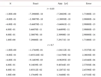
Example 5.1 [7]:

Consider the linear mixed V-FIE with a generalized Cauchy kernel

( )

(

)

(

)

1 ₂

2 2 0 1

1

,t g ,t t , d d

ϕ λ ζ ϕ η ζ η ζ

η

−

ℵ = ℵ +

ℵ −

∫ ∫

(14)

( )

5 6

1.5,N 20, the exact solution ,t t

λ

= =

ϕ

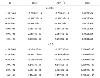
ℵ = ℵ

we obtain Table 1. Example 5.2 [8]:

Consider the nonlinear mixed V-FIE with a generalized Cauchy kernel

( )

(

)

(

)

1 ₂ ₃

2 2 0 1

1

,t g ,t t , d d

ϕ λ ζ ϕ η ζ η ζ

η

−

ℵ = ℵ +

ℵ −

∫ ∫

(15)

( )

5 6

1.5,N 20, the exact solution ,t t

λ

= =

ϕ

ℵ = ℵ

we obtain Table 2.

[image:4.595.207.539.481.734.2]

The results for this examples using the LHPM obtained in Table 1 and Table 2 are best from the results in [7] [8] where the solution was obtained using TMM.

Table 1. Results obtained for example 1 and error.

ℵ Exact App. ( )ϕ Error

t = 0.03

−1.00E+00 −7.29000E−10 −7.28829E−10 1.71000E−13

−8.00E−01 −2.38879E−10 −2.38850E−10 2.90000E−14

−6.00E−01 −5.66870E−11 −5.66841E−11 2.90000E−15

6.00E−01 5.66870E−11 5.66899E−11 2.90000E−15

8.00E−01 2.38879E−10 2.38908E−10 2.90000E−14

1.00E+00 7.29000E−10 7.29171E−10 1.71000E−13

t = 0.7

−1.00E+00 −1.17649E−01 −1.04112E−01 1.35370E−02

−8.00E−01 −3.855120E−02 −3.61709E−02 2.38030E−03

−6.00E−01 −9.14839E−03 −8.90295E−03 2.45440E−04

6.00E−01 9.14839E−03 9.40544E−03 2.57050E−04

8.00E−01 3.85512E−02 4.12071E−02 2.65590E−03

(5)

[image:5.595.209.539.89.346.2]

Table 2. Results obtained for example 2 and error.

ℵ Exact App. ( )ϕ Error

t = 0.03

−1.00E+00 −7.29000E−10 −7.29000E−10 0.0000E+00

−8.00E−01 −2.38879E−10 −2.38879E−10 0.0000E+00

−6.00E−01 −5.66870E−11 −5.66870E−11 0.0000E+00

6.00E−01 5.66870E−11 5.66870E−11 0.0000E+00

8.00E−01 2.38879E−10 2.38879E−10 0.0000E+00

1.00E+00 7.29000E−10 7.29000E−10 0.0000E+00

t = 0.7

−1.00E+00 −1.17649E−01 −1.17573E−01 7.60000E−05

−8.00E−01 −3.85512E−02 −3.85499E−02 1.30000E−06

−6.00E−01 −9.14839E−03 −9.14838E−03 1.10000E−08

6.00E−01 9.14839E−03 9.14840E−03 1.80000E−08

8.00E−01 3.85512E−02 3.85525E−02 1.30000E−06

1.00E+00 1.17649E−01 1.17725E−01 7.60000E−05

6. Conclusion

In this article, we proposed LHPM and used it for solving nonlinear mixed V- FIE with a generalized singular kernel. As examples show, the displayed tech-nique diminishes the computational difficulties of other methods. An interesting feature of this method is that the error is too small and all the calculations can be done straightforward. It can be concluded that LHPM is a very simple, powerful and effective method.

Acknowledgements

The authors would like to thank the king Abdulaziz city for science and tech-nology.

References

[1] Pachpatta, B.G. (1986) On Mixed Volterra-Fredholm Type Integral Equations. In-dian Journal of Pure and Applied Mathematics, 17, 488-496.

[2] Hacia, L. (1996) On Approximate Solution for Integral Equations of Mixed Type.

ZAMM—Journal of Applied Mathematics and Mechanics, 76, 415-416.

[3] Brunner, H. (1990) On the Numerical Solution of Nonlinear Volterra-Fredholm Integral Equation by Collocation Methods. SIAM Journal on Numerical Analysis, 27, 987-1000. https://doi.org/10.1137/0727057

[4] Maleknejad, K. and Hadizadeh, M. (1999) A New Computational Method for Vol-terra-Fredholm Integral Equations. Journal of Computational and Applied Mathe-matics, 37, 1-8. https://doi.org/10.1016/S0898-1221(99)00107-8

(6)

101-127. https://doi.org/10.1016/0898-1221(91)90220-X

[6] Wazwaz, A.M. (1999) A Reliable Modification of Adomian’s Decomposition Me-thod. Applied Mathematics and Computation, 102, 77-86.

https://doi.org/10.1016/S0096-3003(98)10024-3

[7] Abdou, M.A., El-Kalla, I.L. and Al-Bugami, A.M. (2011) Numerical Solution for Volterra-Fredholm Integral Equation with a Generalized Singular Kernel. Journal of Modern Methods in Numerical Mathematics, 2, 1-15.

https://doi.org/10.20454/jmmnm.2011.60

[8] Al-Bugami, A.M. (2013) Toeplitz Matrix Method and Volterra-Hammerstin Integral Equation with a Generalized Singular Kernel. Progress in Applied Mathe-matics, 6, 16-42.

[9] Abdou, M.A., El-Kalla, I.L. and Al-Bugami, A.M. (2011) New Approach for Con-vergence of the Series Solution to a Class of Hammerstein Integral Equations. In-ternational Journal of Applied Mathematics and Computation, 3, 261-269. [10] El-Kalla, I.L. and Al-Bugami, A.M. (2012) Numerical Solution for Nonlinear

Vol-terra-Fredholm Integral Equation with Applications in Torsion Problems. Interna-tional Journal of ComputaInterna-tional and Applied Mathematics, 7, 403-418.

[11] He, J.H. (1999) Homotopy Perturbation Technique. Computer Methods in Applied Mechanics and Engineering, 178, 257-262.

https://doi.org/10.1016/S0045-7825(99)00018-3

[12] He, J.H. (2000) A Coupling Method of a Homotopy Technique and a Perturbation Technique for Non-Linear Problems. International Journal of Non-Linear Mechan-ics, 35, 37-43. https://doi.org/10.1016/S0020-7462(98)00085-7

[13] Abdulaziz, O., Hashim, I. and Chowdhury, M.S.H. (2008) Solving Variational Problems by Homotopy Perturbation Method. International Journal for Numerical Methods in Engineering, 75, 709-721. https://doi.org/10.1002/nme.2279

[14] Golbabai, A. and Keramati, B. (2009) Solution of Non-Linear Fredholm Integral Equations of the First Kind Using Modified Homotopy Perturbation Method.

Chaos, Solitons and Fractals, 39, 2316-2321.

https://doi.org/10.1016/j.chaos.2007.06.120

[15] Ghorbani, A. (2009) Beyond Adomian Polynomials: He Polynomials. Chaos, Soli-tons and Fractals, 39, 1486-1492. https://doi.org/10.1016/j.chaos.2007.06.034

(7)

Submit or recommend next manuscript to SCIRP and we will provide best service for you:

Accepting pre-submission inquiries through Email, Facebook, LinkedIn, Twitter, etc. A wide selection of journals (inclusive of 9 subjects, more than 200 journals)

Providing 24-hour high-quality service User-friendly online submission system Fair and swift peer-review system

Efficient typesetting and proofreading procedure

Display of the result of downloads and visits, as well as the number of cited articles Maximum dissemination of your research work