Ex Post Efficient Set Mathematics
Christopher Adcock
Sheffield University Management School, University of Sheffield, Sheffield, UK Email: [email protected]
ReceivedJanuary 9, 2013; revised February 12, 2013; accepted February 21, 2013
ABSTRACT
This paper considers efficient set mathematics for the case where the covariance matrix of asset returns is assumed known but ex ante the vector of expected returns is replaced by an estimated or forecast value. It is shown that the ex post mean and variance differ from the standard results. Consequently the maximum Sharpe ratio portfolio also differs from the standard result. However, even with uncertainty about the vector of expected returns, subject to the assump- tions made about the joint distribution of actual returns and estimated mean returns, ex post Sharpe ratio maximisers hold the ex post market portfolio. The properties of the zero beta portfolio are similar to the standard results leading to a capital market line. The ex post Capital Asset Pricing Model incorporates an intercept and the betas are not the same as those computed ex ante. The results are illustrated with an example.
Keywords: Beta; CAPM; Efficient Frontier; Efficient Set Mathematics; Market Portfolio; Sharpe Ratio
1. Introduction
Portfolio selection introduced by Markowitz [1] has many supporters and many detractors. Broadly, the former are those who use his methods successfully and the latter are those who do not. Since its introduction, traditional port- folio selection has undergone much refinement and de- velopment. Nonetheless, many of these developments are very similar to or essentially identical to the original method. That is, a portfolio selector remains on a mean- variance efficient frontier. The original theory assumes a quadratic utility function or that the multivariate prob- ability distribution of asset returns is characterized by expected returns and the covariance matrix. Stein’s Lem- ma, Stein [2], and its modern extensions (Liu, [3]; Lands- man and Nešlehová, [4]) mean that these remarks are valid under a range of elliptically symmetric distribu- tions and, subject to regularity conditions, for all utility functions. Thus, the efficient frontier should be a robust place to be.
In the previous paragraph, the phrase “a mean-vari- ance efficient frontier” is used deliberately to remind that in practice all efficient frontiers are based on estimates of the underlying parameters, the vector of expected returns and the covariance matrix. Even when consistent estima- tors of the underlying parameters are used, all efficient frontiers are in reality estimated efficient frontiers. It is well known, by both practitioners and academic re- searchers, that the ex-post performance of an efficient portfolio often differs substantially from that anticipated at the time of construction. The celebrated papers by Best
and Grauer [5] and Chopra and Ziemba [6] document that portfolios which are mean-variance efficient ex ante
are sensitive to the inputs; that is to the estimators that are used. As Adcock [7] reports “even in the situation where the user is equipped with good estimates of the input parameters, the outputs are likely to produce re- sults that are different from those expected. In circum- stances where the estimates of the inputs are poor, it is inevitable that ex-post performance will be inferior”. The recent paper by Kan and Zhou [8] confirms this. These and other difficulties are documented widely, notably in Michaud [9,10].
collectively as efficient set mathematics. Gibbons, Ross and Shanken [14] present a test of the mean-variance efficiency of a portfolio. This test, which employs a fun- damental property of the efficient frontier, is based on a variant of the market model. Under the IID normal as- sumptions, it results in Hotelling’s T2, which apart from a scaling constant has an F distribution. There are similar tests in Huberman and Kandel [15] and Britten-Jones [16]. More recently, Kan and Smith [17] derive expres- sions for the joint distribution of the components of the efficient frontier given the standard assumptions. To achieve this, they reparameterise the frontier and con- sider components which are functions of those in Mer- ton’s original representation. The results that they derive depend on the Chi-squared and non-central F distribu- tions. Knight and Satchell [18] derive further extensions, specifically for institutional investors. There are several other related works, notably by Bodnar and Schmid [19-21], Hillier and Satchell [22] and Okhrin and Schmid [23].
Under the assumption that the vector of expected re- turns and the covariance matrix are known, the ex post or actual return on a portfolio is an affine transformation of the vector of asset returns. If returns follow a multivari- ate normal distribution or any member of the elliptically symmetric class, the distribution of portfolio returns is a member of the same class. The aim of this paper is to present results for the case where the covariance matrix is known, but the vector of expected returns is an esti- mate or forecast and is therefore a random vector. To avoid duplication, henceforth such a vector is referred to as a forecast. When the joint distribution of returns and the forecast used for portfolio selection is multivariate normal, it is shown that the distribution of ex-post portfo- lio returns is an extended quadratic form in normal vari- ables. It is shown that this changes the shape of the effi- cient frontier and leads to different insights into the maximum Sharpe ratio or market portfolio. The results in this paper substantially extend those reported in Adcock [7,24,25].
The paper is set out as follows. Section 2 contains a summary of traditional efficient set mathematics and the assumptions used. Section 3 present the main results of the paper, namely that ex post returns are distributed as an extended quadratic form. Given that the number of possible specifications for the structure of the covariance matrix of asset returns and forecasts is large, Section 4 presents two examples. In Section 5, there are results which examine the effect of the estimated expected re- turns or forecasts on the Sharpe ratio, the market portfo- lio and the Capital Asset Pricing Model. Section 6 con- tains concluding remarks and a brief discussion of poten- tial developments.
2. Traditional Efficient Set Mathematics
Let R be an n-vector of asset returns, which has the multivariate normal distribution N
μ,Σ
. The notationp
R denotes portfolio return and rfthe risk free. The no- tations 0n d 0mn te respectively an n-vector of ones, an n-vector of zeros and an m n m of ze- ros. Subscripts are generally omitted. It is assumed that the covariance matrix Σ is non-singular. Maximising expected utility subject only to the budget constraint in the usual way and recalling Stein’s Lemma, the first or- der conditions for portfolio selection lead to the well known expression for the portfolio weights
1, an deno
atrix
1 1 T
1
T 1 T 1
0 1; 0. θ
1
w μ
w w
Σ 1 Σ Σ 11 Σ
1 Σ 1 1 Σ 1
The vector 0 is the minimum variance portfolio and satisfies the budget constraint . The vector is a self-financing portfolio. In general, risk appetite is defined as
w
T 0 1
w
1 w1
θ
p
p
E U R E U R
The expected return and variance of portfolio return, which has a normal distribution given the assumptions, are
2 2
0 1, 2
p p 1
respectively, where the standard constants are defined as T 1
0 T 1
1 T 1
T 1
1 T 1
2 T 1
,
1 .
μ
μ μ,
Σ 1
1 Σ 1
Σ 11 Σ Σ
1 Σ 1
1 Σ 1
Note that these definitions of the standard constants differ from those in Merton [13]. They are the same as those used in Kan and Smith [17] and are more suitable for the purposes of this paper. The equation of the effi-cient frontier is
2
0 1
p p 2
The market or maximum Sharpe ratio portfolio arises when
2 0 2
M rf 0
,
as long as 0 rf. If 0 rf the market portfolio does not exist in any meaningful sense.
3. Distribution of Portfolio Returns
which it is shown that when μ is replaced by a forecast, denoted by , portfolio return is distributed as an ex- tended quadratic form in normal variables. It is assumed the 2n-vector
F R X F ,
has a non-singular multivariate normal distribution with
,N τ Γ
, RR RF
FR FF μ τ μ δ Σ Σ Γ
Σ Σ ,
respectively. Non-zero entries in the vector mean that the forecast is biased. It is assumed that the covariance matrix is known. The vector of portfolio weights based upon the forecast is
δ
F
1 T 1 1
0 0 0 T 1
w w D F D Σ Σ 11 Σ
1 Σ 1
,
Portfolio return is then
T 21 T p
R b X X AX ,
with 0 0 0 , nn n n θ θ w D b D 0 A
0 0n
.
Portfolio return is distributed as an extended quadratic form in normal variables. The properties of these are described in detail in Mathai and Prevost [26]. Relevant results for financial applications are in Appendix B of Adcock et al [27]. Specifically, Corollary 2 of their Theorem 2 leads to the following.
Proposition 1
Apart from an additive constant, portfolio return Rp
is distributed as the weighted sum of independent non- central Chi-squared variables, each with one degree of freedom, and an independently distributed normal vari- able. That is
2 1 2 0 0 1 , 1 , np j j j
j
R Z
where the λj are the non-zero eigenvalues of the matrix
2 n1
AΓ, 0 and are
scalar functions of elements of the vector τ and the eigenvectors of
, j0,1, , 2 n1
j
AΓ and Zis a standard normal vari- able.
As further technical details of this result are not re- quired for the material that follows below, they are omit- ted. Briefly, it may be noted that the probability density function of Rp is intractable, although the central limit theorem means that, ceteris paribus, the distribution of
p
R will tend to normality as the number of assets in- creases. This provides support to a finding of Tu and
works for the evaluation of portfolio performance. The characteristic function of the extended quadratic form, however, may be inverted numerically using a procedure due to Imhof [29]. Mathai and Prevost [26] note that this procedure may be considered to be exact. The character- ristic function is tractable and leads to the following re- sults for the mean and variance of portfolio returns. An outline proof of the following proposition is in Appendix A. It was first reported without proof in Adcock [25].
Proposition 2
Zhou [28] who suggests that the normality assumption
nd variance of portfolio return, de
2 The expected value a
noted with the additional subscript f, are respectively
0 1 0,
2 2 2
2 1 2 1 ,
pf
pf
and 1
where 0 are
trace
T T
0 D0ΣRF μ D0δ,1μ D0ΣFRw0, and
2
2 0 0 0
T T
0 0 0 0
T T
0 0 0
trace
2 2
RF FF RR
FF RR
RR FR 0
D D D
μ D D μ δ D Dδ
δ D D μ μ D μ δ
Σ Σ Σ
Σ Σ
Σ Σ D .
The covariance between the returns of an arbitrary portfolio with given weights wq and an efficient port- folio with risk appetite θ is
q p
q
θ
RRΣRF
D0μΣRRw0
cov R R, wT ΣSubstitution gives the following:
the efficient frontier is
Corollary 2.1
The equation of
20 1 1
pf A A B pf B0
,
where
0
A 0 1 1 0 1 2 1 1 0
2
0 2 1 1 2 1 1 2
, , , . A B B
From Proposition 2 and Corollary 2.1, it is clear that the ex-post expected return and variance of an efficient portfolio constructed using estimates or forecasts of ex- pected returns are different from those based on standard efficient set mathematics. The effect on the maximum Sharpe ratio portfolio is described in Section 5. The de- tailed effects on mean and variance, and hence the shape of the efficient frontier, depend on the constants 0,1,2. These in turn depend on δ, the bias in the estimates, and the structure of the cova ance matrix Γ. To illustrate the effects, two examples are presented in Section 4.
ri
4. Two Examples
T, T
RR ΗΗ FF ΚΚ
Σ Σ ,
where Η and Κare full rank m trices. The co-
where is the matrix of cross-correlations be- etu fore
In the two examples below, it is assumed that the co- va
n n a variance matrix of returns and forecasts is
T RR
Σ ΗΡΚ
Γ T T ,
FF
ΚΡ Η Σ
Ρ n n
tween r rns and casts. It is convenient to define the following scalars
T 0
1 Η 1 T 1 T 1
1 1 2 RR .
, ,
1 1 Ηw 1 Σ 1
riance matrix of the estimates or forecasts is propor- tional to ΣRR, the covariance matrix of asset returns. This is loo equivalent to assuming that the vector of forecasts is based on simple times series methods. It is also assumed that forecasts are unbiased, δ0.
4.1. Rank One Cross-Correlation M w
sely
atrix ith
In th
Equal Correlations and Unbiased Estimates
is case Ρ11T which leads to T T
T T .
RR Η11 RR Κ Κ Η Σ Γ 11 Σ The constants 0,1,2 are
2
2 1 0 1 2
2 2 2
2 1 0 2 1
,
1 2
n n
0 n 0 ,
.
These are affected by the covariance matrix of asset re
turns through their dependence on Η. Note that 1) by the Cauchy Schwarz inequality 2
2 0
n , expected return is increased (decreased) if is positive 0
t
(negative) and 2) that the requirement tha Γbe positive semi- definite imposes a restriction on .
4.2. Diagonal Cross-Correlat n Mio atrix with s
This
Equal Correlations and Unbiased Estimate
example was first reported in conference proceed-ings in Adcock [24]. In this case ΡI, where I is the n n unit matrix, in which case
, RR R
Σ Σ R
RR RR Γ Σ Σ leading to
0 1 22 1 1
1 , 0,
1 1 2 .
n n
A special case of this is the use of the sample mean returns based on a time series of length T. In this case
1
T
and 0. There is no effect on mean return, but there is an increase in variance. In articular, the is an sing function of the number of as- sets.
To illustrate these results a data set consisting of weekly ret
p
urn 13 FTSE indices is used. The fore- variance
ca
increa
s from
st of the mean returns and the covariance matrix used are shown in Tables A1 and A2 of Appendix C. The illustration considers five values of correlation =
−0.05,−0.01,0,0.01,0.05. The parameter set for cor-responds to sample sizes of T1,5,10,50,100,1000. The value T 1 may be interpreted as meaning t at the covariance matrix associated wit -tive, which corresponds with a sensible practice. The
0,1,2
h pre h the forecasts is dic
and 0,1,2 are computed using the formulae above. These are shown in Table 1. Panel 1) of Table 1
the st constants. Panel 2) shows the com-puted values of 0,1,2
shows andard
corresponding to values of from −0.05 to 0.05. Note that the values of 2 are two orders of magnitude greater than those for 0. In pan 3) the column entitled mult0 shows the multiplier to be applied to the Standard Sharpe ratio. Note t for 0
el
hat
the maximum Sharpe ratio occurs at a lower level of risk than the standard case, but that for 0 the maxim Sharpe ratio portfolio is the minimum variance portfolio (MVP). A graph of the efficient fro for 3 values of um
ntier
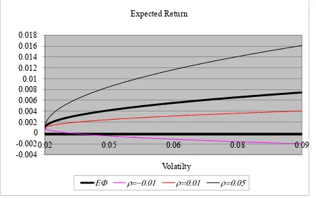
, namely −0.01,0.01and 0.05 and for 1 is shown in Figure 1. The figure also includes a graph of the con-
ntional efficient frontier. As the figure ws, when
ve sho
[image:4.595.307.537.483.734.2] is less than zero the efficient frontier is downwards sloping: more risk leads to lower expected return.
Table 1. Parameters of the efficient frontier.
1) Standard Constants
0.0004 0.0009 0.0057
2) New Components
−0.05 −0.6000 0.0000 12.0351
−0. 0000 12. 8
0.
ters of Efficient Frontier
01 −0.
3
1200 0. 006
0 0.0000 0.0000 12.0057 0.01 0.1200 0.0000 12.0070
05 0.6000 0.0000 12.0363
) Parame
mult0
−0.05 −0.5943 12.0408 −0.0494
−0. 1 −
0.
01 −0.1143 2.0125 0.0095
0 0.0057 12.0114 0.0005
0.01 0.1257 12.0127 0.0105
-0.004 -0.002 0 0.002 0.004 0.006 0.008 0.01 0.012 0.014 0.016 0.018
0.02 0.05 0.06 0.08 0.09
Volatilty Expected Return
[image:5.595.59.289.85.229.2]
Figure 1. The efficient frontier based on forecasts.
For 0.01 the frontier is upwards sloping, but th ient is always less than that for the ex ante effic
e
rad ient
g
frontier. When 0.05, the gradient is higher. That is, this value of correlation provides a sufficient signal to outperform the ex ante frontier. To avoid cluttering the figure other values of are omitted. However, as increases so does the gradient of the frontier. Conversely as decreases from zero, the negative trade-off between risk and expected return becomes progressively worse.
The case 0 may be interpreted as the use of sam- ple returns as a forecast is also omitted. In this case, the corresponding efficient frontier is effectively flat. Figure 2, which is in Section 5, shows the Sharpe ratios plotted against risk appetite θ for the same values of and for the ex ante case.
5. The Sharpe Ratio and the Market
Portfolio
In standard efficient set mathematics, the Sharpe ratio is
20 1 2 1
SR .
For 00 lio is giv
the maximum Sharpe ratio or marke t portfo en by M 2 0. Sectio 5.1 and 5.2 consider t
ns
he Sharpe ratio and the market portfolio for the case when unbiased forecasts of μare used, that is
δ 0. Section 5.3 considers the distribution of returns on the conventional maximum Sharpe ratio portfolio for the c se where the estimate a Fis used in place of μ.
[image:5.595.311.537.85.236.2]5.1. Properties of the Sharpe Ratio
Table 2 shows the differences between the standard ith those when
bi
Sharpe ratio and its properties compared w
the effects of forecasts are taken into account. Specifi- cally, in the rows labeled 1) the table shows the value of θ that maximises the Sharpe ratio, in 2) the value of the Sharpe ratio at the maximum and in 3) the limiting value as θ . The corresponding results for the case of
ased forecasts are substantially more complicated and
-0.05 0 0.05 0.1 0.15 0.2
Sharpe Ratio
0.00 0.40 0.80 1.20 1.60 2.00
Risk Appetite
EF Cor=-0.01 Cor=0.01 Cor=0.05
[image:5.595.307.542.273.431.2]Figure 2. Sharpe ratios based on forecasts. Table 2. Comparison of the sharpe ratio.
Standard
(1) M 2 0
2) 2
1 0
( SRM 2
(3) SR 1
Forecasts
(1) Mf 1 0 M 1 2
2) 2
0 1
( 2
1 2 0 2
M
SR
(3) SRf 1 0 1 2
so are omitted, but are available on request. In the stan- dard c , a necessary and sufficient condition for the aximum Sharpe ratio to exist in a meaningful sense is
ase m
that 00. For the ex post Sharpe ratio the correspond- ing condition is
1 0
0
1 2
0.Mf
Figure 2 shows examples of the Sharpe ratio for =
−0.01, 0.01and 0.05and for . The standard Sharpe ratio is also shown. When = −0.01the max m Shar- pe
r =
arket portfolio under forecast un- lead to
rtfolio is the ex post market portfolio. 1
imu
ratio occurs at the MVP and the ratio declines mono- tonically as risk increases. Fo 0.01 the maximum is close to the MVP and the Sharpe ratio is always inferior to the ex ante case. When = 0.05, however, the Sharpe ratio is superior to the standard case, but the maximum is attained at lower risk.
5.2. The Market Portfolio and the CAPM
The question of the m
certainty naturally arises. Standard manipulations the following.
Proposition 3
Given the assumptions above, the maximum ex post
Thus, although the ex post market portfolio differs fr
he ar
1 om that found ex ante, there is a corresponding capital market line, whose intercept is the risk free rate. T
gument that investors will hold a combination of lend- ing/borrowing and the market portfolio still holds. This is subject to the assumption that the joint distribution of returns and forecasts is the same for all market partici-pants. This result leads in turn to the question of the CAPM. Under the assumptions of the paper, is the ex- pected excess return on an asset or portfolio given by the product of beta and the expected excess return on the market portfolio? The treatment below follows that in Chapter 3 of Huang and Litzenberger [30] and requires the following result.
Proposition 4
The covariance of two efficient portfolios p and q is
cov R Rp, q 2 p q
12
p q
.io with respect to portfolio p if its risk appetite is
This leads to portfolio q being a zero-beta portfol
2 1
1
1 2
z p p
.
Note that for the case where forecasts are biased 1 0
minimu de
and portfolio p may be any portfolio includ g the m variance portfolio. For the case considered in
in
tail in this section, 1 0 and portfolio p can be any io except the minimum variance portfolio. For this case, the expected return on the zero beta portfolio is
portfol
0 2 1 0 1 2
z p
E R
Standard manipulations, similar to those in Chapter 3 of Huang and Litzenberger, lead to the following
Proposition 5
The intercept of the straight line that is the tangent to the efficient frontier at portfolio p is equal to E R
z .Proposition 6
If portfolio p is the market portfolio, the expected re- turn on the zero beta portfolio equals the risk free rate
f r .
In the standard case where μ is given, consideration of the covariance between the returns of portfolio p and
ar
an bitrary portfolio leads to the CAPM if portfolio p is in
portfolio and let
fact the market portfolio. For the case considered in this paper, Proposition 2 leads to a modified version of the CAPM
Proposition 7
Let q be any portfolio with weights wq, M be the ex post market q and M
n δ
be their re-
sp excess ret Whe , it fol-
lo
ective expected urns. 0
ws that
q A B M , where Β
0 1 0 2 1 ,
T
q M q RF M
B w Σ w
where
0 2 0 1 2 , 1 1 0 1 2
.
Note that this reduces to the standard case when μ is given, but that for this case the intercept is not zero general.
in
Continuing the example, Table 3 contains values of alpha and beta for two portfolios for the values of and used above. The first portfolio is an e w
qually eighted portfolio of returns on the 13 FTSE indices. The second is the conventional market portfolio for whic he weights are proportional to 1
RR
h t Σ μ. Panel 1) of
Table 3 shows the alphas and betas for the equally weighted portfolio. These are computed for the standard efficient frontier (table rows called E ey are also computed for the specified values of
F). Th
and . As the table shows, the values of alpha are non-zero. They are numerically small, but of comparable magnitude to the return forecasts shown in appendix Ta A1. T e values of beta decrease as
ble h
increases. Both alpha and beta approach their standard values as decreases to zero, equivalently the implicit sample size increases. Similar behaviour is observed n Panel 2), although it is notable that the alphas are substantial when
i
0.05
. It is also notable that beta is a non-linear function of both and
, with the phenomenon being more apparent for the conventional market portfolio.
3. Property of the Maximum Sharpe Ratio Portfolio
5.
When F is used as the forecast of expected return, maximum Sharpe ratio portfolio has weights given by
the
1 T 1
M RR RR
w Σ F 1 Σ F .
The return on the market portfolio is
T 1 T 1
Mf RR RR
R R Σ F 1 Σ F .
The following interesting result is proved in Appendix B.
Proposition 8
market portfolio based on forecast of the expected
re .
based on estimates may in practice be
considers efficient set mathematics for the case where the covariance matrix of asset returns is as-
Given the assumptions above, the expected value of the
turn is undefined
Strictly speaking, the result is of theoretical interest. Nonetheless, it suggests that returns on the maximum Sharpe ratio portfolio
volatile.
6. Discussion and Concluding Remarks
This paperTable 3. Behaviour of alpha and beta.
Sample Size Equivalent
+1e6 1 10 50 500
(1) Equally weighted portfolio
Alphaq0
EF 0.0000 0.0000 0.0000 0.0000 0.0000
−0.05 0.0004 0.0004 0.0005 0.0006 0.0000
−0.01 0.0004 0.0004 0.0004 0.0000
Betaq0 0.0004
0 0.0004 0.0004 0.0004 0.0003 0.0000
0.01 0.0004 0.0004 0.0003 0.0002 0.0000
0.05 0.0003 0.0003 0.0002 0.0000 0.0000
EF 0.3520 0.3520 0.3520 0.3520 0.3520
−0.05 0.0590 0.0589 0.0595 0.0780 0.4016
−0.01 0.6307 0.6776 7690 1.0027 0.3615
(2) Stan Mark olio
0.
0 0.9988 0.9878 0.9434 0.6832 0.3523
0.01 0.5907 0.5515 0.4916 0.3621 0.3435
0.05 0.0593 0.0600 0.0617 0.0733 0.3114
dard et Portf
Alpham0
EF 0.0000 0.0000 0.0000 0.0000 0.0000
−0.05 0.0142 0.0119 0.0002
−0.01 0.0005 0.0004 0.0000 0.0001
m0
0.0149 0.0155
0.0002
0 0.0000 0.0000 0.0001 0.0004 0.0000
0.01 0.0006 0.0007 0.0009 0.0012 −0.0001
0.05 0.0134 0.0122 0.0097 −0.0015 −0.0003
Beta
EF 1.0000 1.0000 1.0000 1.0000 1.0000
− − −
−0.01 0.6299 0.6771 7743 0.9981 0.9828
0.05 0.0142 0.0794 0.2300 −0.5201 0.9241
0.
0 0.9986 0.9859 0.9358 0.7028 0.9984
0.01 0.5926 0.5599 0.5220 0.5690 1.0144
0.05 0.1059 0.2091 0.4016 1.0876 1.0810
s t ow x an vector of e d
returns i fo a is
th ex post nce d fr
those co
e correlations damage it; volatility
ex
model for the multivariate pr
“Portfolio Selection,” Journal of Finance, Vol. 7, No. 1, 1952, pp. 77-91.
[2] C. M. Stein, “ of a Multivariate
Normal Distri tics, Vol. 9, No. 6,
umed o be kn n but e te the xpecte s replaced
at the by an estimmean and ated or varia recast viffer lue. It om the shown
standard results. Consequently the maximum Sharpe ra- tio portfolio also differs from the standard result. This portfolio remains the market portfolio. Thus, even with uncertainty about the vector of expected returns, subject to the assumptions made about the joint distribution of actual returns and estimated mean returns, ex post Sharpe
ratio maximizers hold the ex post market portfolio. The properties of the zero beta portfolio are also simi- lar to the standard results. A notable exception, however, is that the capital asset pricing model incorporates an intercept and the ex post betas are not the same as
mputed ex ante.
The numerical example provides a demonstration of well-known empirical features: positive correlations be- tween returns and estimates improve ex post portfolio performance; negativ
post may be expected to be higher than that predicted
ex ante.
The assumption of multivariate normality with known covariance matrix is a limitation of the results, except perhaps for those of low frequency. The results presented here imply that a tractable
obability distribution of returns and estimates is re- quired. Scale mixtures of the multivariate normal distri- bution are an obvious candidate. The use of multivariate distributions which incorporate skewness is an open re- search question.
REFERENCES
[1] H. Markowitz,Estimation of the Mean bution,” Annals of Statis
1981, pp. 1135-1151. doi:10.1214/aos/1176345632 [3] J. S. Liu, “Siegel’s Formula via Stein’s Identities,” Statis-
tics and Probability Letters, Vol. 21, No. 3, 1994, pp. 247-251. doi:10.1016/0167-7152(94)90121-X
[4] Z. Landsman and J. Nešlehová, “Stein’s Lemma for El- liptical Random Vectors,” Journal of Multivariate Analy- sis, Vol. 99, No. 5, 2008, pp. 912-927.
doi:10.1016/j.jmva.2007.05.006
[5] M. J. Best and R. R. Grauer, “On the Sensitivity of Mean- Variance-Efficient Portfolios to Changes in Asset Means: Some Analytical and Computational Results,” Review of Financial Studies, Vol. 4, No. 2, 1991, pp. 315-342. doi:10.1093/rfs/4.2.315
[6] V. Chopra and W. T. Ziemba, “The Effect of Errors in Means, Variances and Covariances on Optimal Portfolio Choice,” Journal of Portfolio Management, Vol. 19, No. 2, 1993, pp. 6-11. doi:10.3905/jpm.1993.409440
[7] C. J. Adcock, “Predicting Portfolio Returns Using The Distributions of Efficient Set Portfolios,” In S. E. Satchell and A Scowcroft, Eds., Advances in Portfolio Construc- tion and Implementation, Butterworth Heinemann, Ox- ford, 2003, pp. 342-355.
[8] R. Kan and G. Zhou, “Optimal Portfolio Choice with Parameter Uncertainty,” Journal of Financial and Quan- titative Analysis, Vol. 42, No. 3, 2007, pp. 621-656. doi:10.1017/S0022109000004129
pp. 31-42.
[10] R. O. Michaud, “Efficient Asset Management,” Harv Business School Press, Boston, 1998. ard
h Holland, Amsterdam, Vol. 3, 1979.
merican Statistical [11] V. Bawa, S. J. Brown and R. Klein, “Estimation Risk and
Optimal Portfolio Choice,” Studies in Bayesian Econo- metrics, Nort
[12] J. D. Jobson and B. Korkie, “Estimation for Markowitz Efficient Portfolios,” Journal of the A
Association, Vol. 75, No. 371, 1980, pp. 544-554. doi:10.1080/01621459.1980.10477507
[13] R. Merton, “An Analytical Derivation of the Efficient Portfolio Frontier,” Journal of Financial and Quantitative Analysis, Vol. 7, No. 4, 1972, pp. 1851-1872.
doi:10.2307/2329621
[14] M. R. Gibbons, S. A. Ross and J. Shanken, “A Test of the Efficiency of a Given Portfolio,” Econometrica, Vol. 57, No. 5, 1989, pp. 1121-1152. doi:10.2307/1913625 [15] G. Huberman and S. Kandel, “Mean-Variance
The Journal of Financ
Spanning, e, Vol. 42, No. 4, 1987, pp.
873-”
888. doi:10.1111/j.1540-6261.1987.tb03917.x
[16] M. Britten-Jones, “The Sampling Error in Estimates of Mean-Variance Efficient Portfolio Weights”. Journal of Finance, Vol. 54, No. 2, 1999, pp. 655-672.
doi:10.1111/0022-1082.00120
[17] R. Kan, and D. R. Smith, “The Distribution of the Sample Minimum-Variance Frontier,” Management Science, Vol. 54, No. 7, 2008, pp. 1364-1360.
doi:10.1287/mnsc.1070.0852
[18] J. Knight, and S. E. Satchell, “Exact Properties of Meas-ures of Optimal Investment for Benchmarked Portfolios,” Quantitative Finance, Vol. 10, No. 5, 2010, pp. 495-502. doi:10.1080/14697680903061412
[19] T. Bodnar, and W. Schmid, “A Test for the Weights of the Global Minimum Variance Portfolio in an Elliptical Model,” Metrika, Vol. 67, No. 2, 2008, pp. 127-143. doi:10.1007/s00184-007-0126-7
[20] T. Bodnar and W. Schmid “Estimation of Optimal Portfo-lio Compositions for Gaussian Returns,” Statistics & De-cisions, Vol. 26, No. 3, 2008, pp. 179-201.
doi:10.1524/stnd.2008.0918
[21] T. Bodnar and W. Schmid “Econometrical Analysis of the Sample Efficient Frontier,” The European Journal of Fi-nance, Vol. 15, No. 3, 2009, pp. 317-335.
doi:10.1080/13518470802423478
[22] G. H. Hillier and S. E. Satchell, “Some Exact Results for Efficient Portfolios with Given Returns,” In S. E. Satchell and A Scowcroft, Eds., Advances in Portfolio Construc-tion and ImplementaConstruc-tion, Butterworth Heinemann, Ox-ford, 2003, pp. 310-325.
[23] Y. Okhrin and W. Schmid, “Distributional Properties of Portfolio Weights,” Journal of Econometrics, Vol. 134, No. 1, 2006, pp. 235-256.
doi:10.1016/j.jeconom.2005.06.022
[24] C. J. Adcock, “The Statistical Properties of Optimised Portfolios,” Proceedings of the 1996 Chemical Bank— Imperial College Conference on Forecasting Financial Markets, London, 1996.
[25] C. J. Adcock, “Dynamic Control of Risk in Optimised Portfolios,” The IMA Journal of Mathematics Applied in Business and Industry, Vol. 11, No. 1, 2000, pp. 27-138. [26] M. Mathai and S. B. Prevost, “Quadratic Forms in Ran-
dom Variables,” Springer, Heidelberg, 1992.
[27] C. J. Adcock, M. C. Cortez, M. R. Armada and F. Silva “Time Varying Betas and the Unconditional Distribution of Asset Returns,” Quantitative Finance, Vol. 12, No. 6, 2012, pp. 951-967. doi:10.1080/14697688.2010.544667 [28] J. Tu and G. Zhou, “Data-Generating Process Uncertainty:
What Difference Does It Make in Portfolio Decisions?” Journal of Financial Economics, Vol. 72, No. 2, 2004, pp. 385-421. doi:10.1016/j.jfineco.2003.05.003
[29] J. P. Imhof, “Computing the Distribution of Quadratic Forms in Normal Variables,” Biometrika, Vol. 48, No. 3, 1961, pp. 419-426.
[30] C.-F. Huang and R. H. Litzenberger, “Foundations for Financial Economics,” Prentice Hall, Englewood Cliffs, 1988.
Appendices
Table A1. Forecast Mean Weekly Returns for 13 FTSE Indices.A—Moments of Extended Quadratic Forms in
Normal Variables No. Index Forecast
1 FTSE100 0.0012
2 FTSE250 0.0017
3 FTS250-ex-Inv 0.0017
4 FTSE350 0.0013
5 FTSE350-ex-Inv 0.0013
6 FTSE350-HY 0.0013
7 FTSE350-LY 0.0011
8 FTSE-SC 0.0012
9 FTSE-Sex-Inv 0.0010
10 FTSE-All-Share 0.0013
11 FTSE-AS-ex-Inv 0.0013
12 FTSE-AS-ex-mult 0.0011
13 FTSE-Aim 0.0006
In the notation of section 3, portfolio return is T 21 T
p
R b X X AX
This may be written as the quadratic form 1 T
2 p
R X AX ,
where
,
X A I
X A
b I
0 .
The vector X has a singular multivariate normal dis- tribution with mean vector and covariance matrix
,
τ τ
b
Γ Γ 0
0 0 ,
respectively. For a random vector which has the gen-eral multivariate normal distribution standard results are that the cumulants of the quadratic form
are
Y
N
μ,Σ
,,
T
[image:9.595.307.538.112.324.2]Y BY
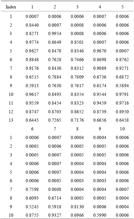
Table A2. Sample Covariance/Correlation Matrix.
1 T
2k 1 ! trace k k
k k k
ΣB μ B μ
where Β 1 Β Β, 2 Β ΒΣ and so on, and that
T T
Tcov d Y Y BY, d ΣBμ.
Substitution of , τ Γ, A and gives the results of Proposition 2. q
w
B—Proof of Proposition 8
The return on the market portfolio is
T 1 T 1
Mf RR RR
R R Σ F 1 Σ F, where and have the
multivariate normal distribution as defined in Section 3. Conditional on
R
N τ
F
,Γ
F f , the expected value of is
Mf
R
T 1 1 T 1 T 1 .
RR RF RF RF
f Σ μ Σ μ δ f Σ f f Σ 1
Index 1 2 3 4 5
1 0.0007 0.0006 0.0006 0.0007 0.0006
2 0.8440 0.0007 0.0008 0.0006 0.0006
3 0.8271 0.9954 0.0008 0.0006 0.0006
4 0.9774 0.8649 0.8501 0.0007 0.0006
5 0.9627 0.8478 0.8346 0.9670 0.0007
6 0.8848 0.7628 0.7466 0.8698 0.8762
7 0.9176 0.8430 0.8312 0.9089 0.9271
8 0.6515 0.7884 0.7809 0.6736 0.6872
9 0.5913 0.7630 0.7617 0.6174 0.5894
10 0.9617 0.8493 0.8354 0.9544 0.9791
11 0.9559 0.8454 0.8323 0.9459 0.9716
12 0.8747 0.8703 0.8652 0.8739 0.8950
13 0.6445 0.7265 0.7176 0.6656 0.6458
6 7 8 9 10
1 0.0006 0.0007 0.0004 0.0004 0.0006
2 0.0005 0.0006 0.0005 0.0005 0.0006
3 0.0005 0.0007 0.0005 0.0005 0.0006
4 0.0006 0.0007 0.0004 0.0004 0.0006
5 0.0006 0.0007 0.0004 0.0004 0.0006
6 0.0006 0.0005 0.0003 0.0003 0.0006
7 0.7598 0.0008 0.0004 0.0004 0.0007
8 0.6093 0.6714 0.0005 0.0005 0.0004
9 0.5245 0.5918 0.8130 0.0006 0.0004
10 0.8755 0.9327 0.6966 0.5990 0.0006
The first term is the ratio of two variables which have a bivariate normal distribution. Cedilnik, Košmelj and Blejec [31] show that such a variable does not have an expected value or higher moments. This is sufficient to ensure that the unconditional moments of RMf are un- defined.
[image:9.595.307.539.352.730.2]Continued
11 0.8667 0.9254 0.6903 0.5934 0.9701
12 0.8206 0.8403 0.7181 0.6468 0.8943
13 0.5298 0.6745 0.7548 0.7508 0.6617
11 12 13
1 0.0006 0.0006 0.0004 2 0.0006 0.0006 0.0005 3 0.0006 0.0006 0.0005 4 0.0006 0.0006 0.0004 5 0.0006 0.0006 0.0004 6 0.0006 0.0005 0.0003 7 0.0007 0.0006 0.0005 8 0.0004 0.0004 0.0004 9 0.0004 0.0004 0.0005 10 0.0006 0.0006 0.0004 11 0.0007 0.0006 0.0004 12 0.8896 0.0007 0.0004 13 0.6472 0.6434 0.0006