Munich Personal RePEc Archive
Improving bias in kernel density
estimation
Mynbaev, Kairat and Nadarajah, Saralees and Withers,
Christopher and Aipenova, Aziza
Kazakh-British Technical University„ School of Mathematics,
University of Manchester, Applied Mathematics Group, Industrial
Research Limited„ Kazakh National University,
2014
Online at
https://mpra.ub.uni-muenchen.de/75846/
Improving bias in kernel density estimation
Kairat T. Mynbaeva,1,∗, Saralees Nadarajahb, Christopher S. Withersc, Aziza S. Aipenovad
aKazakh-British Technical University, Almaty 050000, Kazakhstan bSchool of Mathematics, University of Manchester, Manchester M13 9PL, UK cApplied Mathematics Group, Industrial Research Limited, Lower Hutt, New Zealand
dKazakh National University, Almaty, Kazakhstan
Abstract
For order q kernel density estimators we show that the constant bq in bias =
bqhq+o(hq) can be made arbitrarily small, while keeping the variance bounded.
A data-based selection ofbq is presented and Monte Carlo simulations illustrate
the advantages of the method.
Keywords: density estimation, bias, higher order kernel
2010 MSC: 62G07, 62G10, 62G20
1. Introduction
Letf denote a density,K an integrable function onRsuch thatR
Kdt= 1 and letX1, ..., Xn be i.i.d. random variables with densityf. Consider the kernel
estimator off(x)
fh(x, K) =
1
n
n
X
j=1 1
hK
x−Xj
h
, h >0. (1)
Denote αi(K) = R xiK(x)dx the ith moment of K and let K be a kernel of
orderq, that isαj(K) = 0,j= 1, ..., q−1, αq(K)6= 0. It is well-known that the
∗Corresponding author
Email addresses: [email protected](Kairat T. Mynbaev),
[email protected](Saralees Nadarajah),[email protected]
(Christopher S. Withers),[email protected](Aziza S. Aipenova)
bias is proportional toαq(K)hq iff is q-smooth in some sense [Devroye, 1987,
Scott, 1992, Silverman, 1986, Wand & Jones, 1995].
The usual approach is to stick to someKand be content with the resulting
αq(K). The purpose of this paper is to show that it pays to reduceαq(K) by
choosing a suitable K. Despite the bias being proportional to αq(K)hq, the
benefits of the suggested approach are not obvious because as theqth moment is made smaller, the variance of the estimator may go up. Our construction of
K allows us to control the variance. Our results imply that among all kernels of order q with uniformly bounded variances there is no kernel with the least nonzero|αq(K)|. The issue of selecting the kernel order does not arise in the
approach suggested in [Mynbaev and Martins Filho, 2010].
In case of L1 convergence the main idea can be illustrated using the corre-sponding bias notion from Devroye [1987]. Let bias be defined asR
|f ⋆Kh−f|dt
whereKh(x) =K(x/h)/h. IfK is of orderq,f hasq−1 absolutely continuous
derivatives and an integrable derivativef(q), then by [Devroye, 1987, Theorem 7.2]
q!
Z
|f ⋆ Kh−f|dt/
hq
Z
|f(q)|dt
→αq(K), h↓0.
Hereαq(K) can be made as small as desired using our Theorem 2.
We call a free-lunch effect the fact that αq(K) can be made as small as
desired, without increasing the density smoothness or the kernel order. Of
course, in finite samples bias cannot be eliminated completely. Put it differently,
for very smallαq(K) sample variance starts to dominate the effect of small bias.
For simplicity, in our main results in Section 2 we consider only classical
smoothness characteristics. The simulation results in Section 3 compare our
kernel performance with that of three well-known kernel families. The overall
conclusion is that a better estimation performance is not necessarily a
conse-quence of some optimization criterion and can be achieved by directly targeting
2. Main results
Multiplication by polynomials [Deheuvels, 1977, Wand & Schucany, 1990] is
one of several ways to construct higher-order kernels. [Withers and Nadarajah,
2013] have explored the procedure of transforming a kernelKinto a higher-order kernel TaK via multiplication of K by a polynomial of order q, (TaK)(t) =
Pq
i=0aiti
K(t), with a suitably chosen vector of coefficientsa= (a0, ..., aq)′∈
Rq+1. Unlike several authors who chose the polynomial subject to some opti-mization criterion (see [Berlinet, 1993, Fan & Hu, 1992, Gasser & Muller, 1979,
Lejeune and Sarda, 1992, Wand & Schucany, 1990]) Withers & Nadarajah with
their definition of the polynomial directly targeted moments of the resulting
kernel. In their Theorem 2.1, they defined a polynomial transformation in such
a way that the moments of the new kernel numbered 1 throughq−1 are zero. They did not notice that theqth moment can be targeted in the same way and can be made as small as desired and that the variance of the resulting estimator
retains the order 1/(nh) as theqth moment is manipulated. This is what we do here. Besides, we show that not only variance but all the higher-order terms in
hin the Taylor decomposition of the bias and variance can be controlled not to increase.
We do this under two sets of assumptions. The first set is that the density
is infinitely differentiable and all moments ofKexist and the second is that the density has a finite number of derivatives and the kernel and its square possess
a finite number of moments. We give complete proofs for the first set, because
part of the argument is new and it can be extended to justify some formal
infinite decompositions from [Withers and Nadarajah, 2013]. The proof for the
second set goes more along traditional lines (except for controlling higher-order
terms) and is therefore omitted.
Let βj(K) = RR|K(t)tj|dt denote the jth absolute moment of K. The
estimator off(l)(x) is obtained by differentiating both sides of (1)l times.
Theorem 1. Suppose thatf is infinitely differentiable andK has a continuous
of all orders, lim sup j→∞
f(j)(x)
j! max
βj+1(K), βj+1(K(l))
1/j
= 0, (2)
K
(l) C(
R)= supt∈R K
(l)(t)
<∞. (3)
Then
Efh(l)(x, K) =
∞ X
i=0
f(i+l)(x)
i! (−h)
iα
i(K), (4)
varfh(l)(x, K)= 1
nh2l+1
(∞ X
i=0
f(i)(x)α
i(M)
i! (−h)
i−hhhlEf(l)
h (x, K)
i2 )
(5)
whereM =
K(l)2
and the series converge for allh∈R. Consequently, ifK is a kernel of orderq, then
Efh(l)(x, K)−f(l)(x) = f(q+l)(x)
q! (−h)
qα
q(K) +O(hq+1), (6)
varfh(l)(x, K) = 1
nh2l+1
f(x)
Z
R
M(t)dt+O(h)
. (7)
Further, for the ISE convergence of the estimator of thelth derivative off the asymptotically optimal bandwidth is given by
hopt=
(
(2l+ 1)α0((K(l))2) 2qnα0(f(q+l))2
q!
αq(K)
2)1/(2q+2l+1)
. (8)
With the functionK we can associate symmetric matrices
Aq(K) =
α0(K) α1(K) ... αq(K)
α1(K) α2(K) ... αq+1(K)
... ... ... ... αq(K) αq+1(K) ... α2q(K)
, Bq=Aq(K2).
In the next theorem we prove the free-lunch effect, for simplicity limiting
Theorem 2. Suppose that f is infinitely differentiable, K is continuous and has absolute moments of all orders,kKkC(R)<∞,
lim sup
j→∞
f(j)(x)
j! βq+j+1(K)
1/j
= 0, (9)
detAq(K) 6= 0. (10)
Let a vectorb∈Rq+1 have components b0= 1, b1=...=bq−1= 0, bq >0 and
seta=Aq(K)−1b. Then
Efh(x, TaK)−f(x) =
f(q)(x)
q! (−h)
qb
q+O(hq+1), (11)
var(fh(x, TaK)) = 1
nh{f(x)b
′
Cqb+O(h)} (12)
whereCq =Aq(K)−1BqAq(K)−1andb′Cqb>0.The terms of higher order in
hin (11)and (12)retain their magnitude as bq→0.
Remark 1. Taking 0 < m < q, b0 = ... = bm−1 = bm+1 = ... = bq−1 = 0,
bm= 1,bq6= 0 we obtain an (m, q)-kernel, see the related definitions and theory
in [Berlinet & Thomas-Agnan, 2004].
Corollary 1. Denote the elements of Aq(K)−1 by Aijq, i, j = 0, ..., q, c =
(1,0, ...,0)′ ∈
Rq+1 andd= (0, ...,0, bq)′ ∈
Rq+1. Thenb=c+d. As bq →0,
one has (TaK)(t) →
Pq
i=0Ai,q0ti
K(t), b′C
qb=c′Cqc+O(bq)→(Cq)11 =
P
i,jAi,q0(Bq)ijAj,q0. It follows that in (11)bq can be made as small as desired,
while (12)retains its magnitude as we do this.
Remark 2. In the course of the proof of Theorem 2 we show that Bq is
pos-itive definite. The argument can be adapted to show that (10) holds if K is nonnegative.
SinceTaK,the optimal bandwidth and the minimized value of the asymp-totic ISE all depend on the numberbq in (11), application of the optimal
band-width (8) is not straightforward. We find it more convenient to discuss the
choice ofbq in the simulations section.
In the next theorem we give conditions sufficient for the free-lunch effect
Kernel family q=2 q=4 q=6 q=8 q=10 q=12 Epanechnikov 0.2000 -0.0476 0.0117 -0.0029 0.0007 -0.0002
Gram-Charlier 1 -3 15 -105 945 -10395
Table 1: Moments of two types of kernels
Theorem 3. Suppose that (10) holds, f is (q+ 1)-times continuously
differ-entiable,kf′k
C(R)+
f(q+1)
C(
R)<∞and β2q+1(K) +β2q+1(K
2)<∞. Then (11)and (12)are true. For the ISE convergence the optimal bandwidth is given
by (8) wherel= 0.
3. Monte Carlo simulations
3.1. Description of kernel families and target densities
We focus on the category of kernels obtained from second-order kernels by
multiplying by polynomials, because our estimator is in this category. This
type of kernel construction is also known to be computationally efficient. For
the purpose of comparison with our kernels, we select two classes of kernels. One
is based on the Gaussian kernel and the other extends Epanechnikov’s approach.
We take the two families from [Berlinet & Thomas-Agnan, 2004].
Epanechnikov-type kernels are given in [Berlinet & Thomas-Agnan, 2004,
p.142]. The entry for the 8th order should look like this: (11025−132300x2+ 436590x4−540540x6+ 225225x8)/4096. Outside the segment [−1,1] the kernels are zero, inside the segment they are defined by the formulas in that table.
The Gram-Charlier kernels are taken from [Berlinet & Thomas-Agnan, 2004,
p.140]. The entry for the 8th order has also been corrected to (105−105x2+ 21x4−x6)/48φ(x). The corrections are based on equations from [Berlinet & Thomas-Agnan, 2004, p.162] implemented in Mathematica. Here φ(x) is the Gaussian density. All these kernels have even orders, and we also use only even
orders. The moments of the kernels of two types are given in Table 1.
The target densities, that is the densities to be estimated, are those proposed
1. Gaussian (f1(x)≡N(0,1)),
2. Bimodal (f2(x)≡N(−1,4/9)/2 +N(1,4/9)/2),
3. Separated-Bimodal (f3(x)≡N(−1.5,1/4)/2 +N(1.5,1/4)/2) and 4. Trimodal (f4(x)≡(9N(−6/5,9/25) + 9N(6/5,9/25) + 2N(0,1/16))/20).
They are listed in the order of increasing curvature, the Trimodal being the
most difficult to estimate.
3.2. Bandwidth choice
Equations (6) and (7) imply thatISE=R
(var+bias2)dxasymptotically is
φ(h) where
φ(h) =c1h2q+c2h−(2l+1), c1=
αq(K)
q!
2Z
f(q+l)2dx, c2= 1
n
Z
K(l)2dx.
(13)
Minimizingφwe obtain
hopt=
(2l+ 1)c2 2qc1
1/(2q+2l+1)
(14)
from which the usual expression for the optimal bandwidth (8) obtains.
In what follows we consider only estimation of densities (l= 0).In this case the minimized value ofφis
φ(hopt) =c11/(2q+1)c
2q/(2q+1)
2 (2q+ 1)(2q)
−2q/(2q+1). (15)
For conventional kernels the constantsc1, c2 are given by (13) withl = 0 and in case ofTaK we have functions ofbq
c1(bq) =
b
q
q!
2Z
f(q)2dx, c2(b
q) =
1
nb
′
Cqb. (16)
Plugging (16) in (14) we obtain definitions ofhopt(bq). Substitutinghopt(bq) in
(15) we obtainφ(hopt(bq)).
Obviously, (15) tends to zero asbq →0. However, settingbq = 0 would not
eliminate bias completely. There is a general fact that for kernel estimators
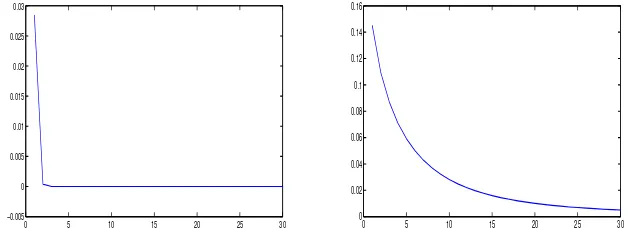
p.113]. In our situation, we illustrate this fact in Figure 1, which depicts the
behavior of average bias and MSE as functions ofbq. Both increase as bq →
0. (Note: in Figure 1, average bias is the average over iterations of integrals
R
(f(x)−fˆ(x, bq))dx for each value of bq; f(x), fˆ(x, bq) are a density and its
estimator, resp.). Whenbq →0, the ”optimal” bandwidth (14) tends to infinity.
The estimator becomes oversmoothed, thus the behavior of average bias and
MSE observed in Figure 1.
0 5 10 15 20 25 30
−0.005 0 0.005 0.01 0.015 0.02 0.025 0.03
0 5 10 15 20 25 30
[image:9.612.147.462.273.396.2]0 0.02 0.04 0.06 0.08 0.1 0.12 0.14 0.16
Figure 1: Left pane: average bias. Right pane: Mean Squared Error. In both panes the
bq values are the values on the x axis times 2×10⁻⁴. The numbers of observations and repetitions are 1000; the density is Gaussian, and the transformed kernelTaK is of order 2
based on the Epanechnikov family.
The choice ofbq should reflect the trade-off between the free-lunch effect and
estimator variance in finite samples. In case of conventional kernels, this
trade-off is incorporated in the optimal bandwidth, and the bandwidth choice ends
there. Here we discuss two approaches we tried in our simulations: I) in onebq
is proportional toαq(K) with some scaling coefficientm, that is, bq =mαq(K)
and II) the other is based on comparison of minimized values of ISE (this was
the suggestion of one of the reviewers). After a lot of experimenting we found
that in fact Approach I works forq= 2, q= 4 givingm= 0.25, while Approach II is better for q ≥ 6 giving m = 0.4. The following is the summary of our experiments.
bq =mαq(Kq) with some multiplier m. With this idea in mind, we looked at
empirical ISE for conventional kernels. It turned out that for small sample
sizes (around 100) the theoretical optimal bandwidth was not so optimal. The
best bandwidth was about 0.4hopt. For large sample sizes (around 1000) the
empirical ISE was flat in a large interval around the theoretical optimalh.That large interval contained the number 0.4hopt. Thus, 0.4hoptwas at least as good
ashopt in our simulations for all sample sizes and all conventional kernels. By
analogy we setm= 0.4 forTaK.This choice turned out to be robust with respect to the choice of the estimated density. Unfortunately, estimation results with
TaK were strictly better than with conventional kernels only for kernel orders
q = 6,8,10,12. In cases q = 2, q = 4 the transformed kernel with m = 0.4 was about as good as the conventional ones, and to find a better multiplier we
turned to the second approach.
Approach II.Here we explore the idea to choosebq satisfying
φ(hopt(bq))≤φ(hopt), (17)
see the definitions in the beginning of Section 3.2. Plugging the numbers from
(16) and (15), resp., into (17) and canceling out common factors (they depend
only onn, q andf(q)) we obtain an equivalent condition
bq(b′Cqb)q≤ |αq(Kq)| α0(Kq2)
q
. (18)
The notationKqis used to emphasize thatKdepends onq.Luckily, this
condi-tion does not involve the density to be estimated. The left side is a polynomial
ofbq of degree 2q+ 1. By Corollary 1 this polynomial is of order O(bq) in the
neighborhood of zero and (18) always holds for all smallbq.However, selecting
bq very small or zero is not an option because of the estimator oversmoothing
problem illustrated in Figure 1.
Denote maxbq the largest positivebq satisfying (18). Here we consider only
q= 2, q= 4. We tried to see if setting bq to maxbq would work. For
Gram-Charlier kernels the values of maxbq were 1 (q= 2) and 0.7612 (q = 4). For
Of these numbers, only 0.7612 worked well. Note that for the Gram-Charlier kernel of order 4 one hasαq(K) = 3, and the number 0.7612 is approximately
0.25αq(K). This suggests the choicem= 0.25. Surprisingly, the multiplierm=
0.25 worked well for all kernels considered in this paragraph (Gram-Charlier and Epanechnikov of ordersq= 2, q= 4), which ended our multiplier selection. Just as a side remark, we explain why the second approach could not be
used for allq.
1) The values of maxbq behave too irregularly to be useful.
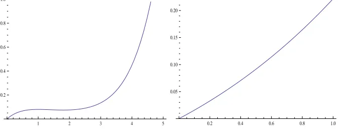
2) Another difficulty is that the polynomialbq(b′Cqb)q may not be strictly
monotone in the interval between zero and the upper bound. For instance, for
Gram-Charlier kernels of orders 2, 6, 10 the derivative of the said polynomial has
positive (sometimes double) roots, while the remaining kernels (of orders 4, 8,
12) are monotone, see Figure 2. Picking an arbitrarybqbetween zero and maxbq
1 2 3 4 5
0.2 0.4 0.6 0.8 1.0
0.2 0.4 0.6 0.8 1.0 0.05
[image:11.612.138.474.379.509.2]0.10 0.15 0.20
Figure 2: Graphs ofhoptas a function ofbq. Left pane: q= 2. Right pane:q= 4
may not provide the right balance between bias and variance. In simulations we
found excellent choices for all kernel orders but could not formulate a general
rule for selecting on ”optimal”bq.
Summarizing, the ”best” values ofbqarebq =mαq(Kq) where the multiplier
mis 0.25 for q = 2, q= 4 andm = 0.4 for the remaining orders. The results reported in the next section are based on these values. After having made these
even better in that case (the statistics are not reported to preserve space). Fan
and Hu kernels are similar to Gram-Charlier in the sense that both families are
based on the Gaussian densityφ(x). To show how different they are, we are giving the expression for the Fan and Hu kernel of orderq = 8: φ(x)(40320−
282240x2+ 352800x4−147840x6+ 26145x8−2121x10+ 77x12−x14)/5040 (the corresponding Gram-Charlier kernel is obtained by multiplying the polynomial
given in Section 3.1 byφ(x)).
Finally, we compared all four families of kernels: our kernels are the best, if
the multiplier is chosen as indicated, Epanechnikov is the second best, followed
by Gram-Charlier, which is followed by Fan and Hu. However, our simulations
do not guarantee that our multiplier choice will deliver improvement over any
other kernel family.
3.3. Estimation results
Let us say we want to estimate the trimodal density. With the chosen sample
size, we estimate it twice: once using the conventional kernel and then using its
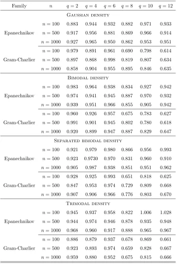
rivalTaK(of the same order and based on the kernel from the same family; the multiplier value is either 0.25 or 0.4). This is repeated 1000 times and the Mean Squared Error (MSE) for the transformed kernel is divided by the MSE for the
conventional kernel, to see the percentage gain/loss. The results are reported
in Table 2.
It is evident that the relative performance of the proposed kernels improves
as the sample size and kernel order grow. The improvement ranges from 5%
to 30% in the lower right corner of each subtable (where n = 1000 and q = 12). The improvement over Gram-Charlier kernels is much larger than over
Epanechnikov ones. The overall conclusion is that the proposed method delivers
Family n q= 2 q= 4 q= 6 q= 8 q= 10 q= 12
Gaussian density
n= 100 0.883 0.944 0.932 0.882 0.971 0.933 Epanechnikov n= 500 0.917 0.956 0.881 0.869 0.966 0.914
n= 1000 0.927 0.965 0.950 0.862 0.953 0.951
n= 100 0.979 0.891 0.961 0.690 0.798 0.614 Gram-Charlier n= 500 0.897 0.868 0.998 0.819 0.807 0.634
n= 1000 0.858 0.904 0.955 0.895 0.846 0.635
Bimodal density
n= 100 0.983 0.964 0.938 0.834 0.927 0.942 Epanechnikov n= 500 0.974 0.941 0.945 0.887 0.970 0.932
n= 1000 0.939 0.951 0.966 0.855 0.905 0.942
n= 100 0.960 0.926 0.957 0.675 0.783 0.627 Gram-Charlier n= 500 0.991 0.901 0.945 0.802 0.780 0.618
n= 1000 0.920 0.899 0.947 0.887 0.829 0.647
Separated bimodal density
n= 100 0.921 0.979 0.980 0.866 0.956 0.993 Epanechnikov n= 500 0.923 0.9730 0.970 0.831 0.960 0.910
n= 1000 0.905 0.987 0.938 0.851 0.951 0.962
n= 100 0.928 0.925 0.993 0.651 0.818 0.625 Gram-Charlier n= 500 0.847 0.953 0.974 0.729 0.809 0.668
n= 1000 0.907 0.906 0.966 0.776 0.803 0.670
Trimodal density
n= 100 0.945 0.937 0.958 0.822 1.006 1.028 Epanechnikov n= 500 0.944 0.974 0.946 0.878 0.935 0.948
n= 1000 0.968 0.960 0.917 0.888 0.965 0.967
n= 100 0.886 0.879 0.937 0.678 0.869 0.661 Gram-Charlier n= 500 0.923 0.893 0.974 0.659 0.828 0.667
[image:13.612.133.488.124.653.2]n= 1000 0.959 0.880 0.952 0.675 0.815 0.666
4. Proofs
By c1, c2, ... we denote various positive constants whose precise value does not matter.
Lemma 1. Under condition (2)
lim sup
j→∞ f
(j)(x)/j!
1/j
= 0, (19)
f(k)(x+h) =
∞ X
i=0
f(i+k)(x)
i! h
i, k= 0,1,2, ... (20)
where all the series converge for anyh∈R.
Proof. We start with a simple generalization of inequality (1.4.7) from [Lukacs,
1970]. Let 1≤i < j <∞.By H¨older’s inequality with p=j/i, 1/q+ 1/p= 1 we have
Z K(t)ti
dt ≤
Z
|K(t)|dt
1/qZ
|K(t)| |t|ipdt
1/p
≤
Z
|K(t)|dt
(j−i)/jZ K(t)tj
dt
i/j
or [βi(K)]1/i ≤[β0(K)]1/i
−1/j
[βj(K)]1/j. Fori, j in the range under
consider-ation one has 0<1/i−1/j <1,so the above inequality implies
[βi(K)]1/i≤cK[βj(K)]1/j for all 1≤i < j <∞ (21)
wherecK = max{1, β0(K)}.This bound yields 1≤c1βj(K)1/j.Using also (2)
we see that (19) is true. By the Cauchy-Hadamard theorem then the series
f(x+h) = P∞
i=0f(i)(x)hi/i! converges for any h ∈ R. By the properties of power series all the series (20) converge.
Lemma 2. If βi(K) +βi(K(l)) < ∞, then for j = 0,1, ..., l −1 one has
sups∈R
K(j)(s)si
≤c1βi(K) +βi(K(l)).
Proof. Lets >0.It is well-known that the Sobolev spaceWl
1[0,1] is embedded inCj[0,1] forj= 0,1, ..., l−1,that is, with some constantc
one has K(j)
C[0,1] ≤c2R 1 0
|K(t)|+|K(l)(t)|
dt.Applying this bound to the segment [s, s+ 1] and using the fact that|t/s|i≥1 fort∈[s, s+ 1] we obtain
K
(j)(s)
≤ c2 Z s+1
s
h
|K(t)|+|K(l)(t)|idt
≤ c2
|s|i
Z s+1
s
h
|K(t)|+|K(l)(t)|i|t|idt≤ c2 |s|i
h
βi(K) +βi(K(l))
i
.
The cases <0 is treated similarly. This proves the lemma.
Lemma 3. If condition (2)holds, we have the representationR
RK(−s)f
(l)(x+
sh)ds=P∞
i=0f(i+l)(x)αi(K)(−h)i/i!.
Proof. Substitutingf(l)(x+sh) from (20) and changing the order of integration and summation produces
Z
R
K(−s)f(l)(x+sh)ds = Z
R
K(−s)
∞ X
i=0
f(i+l)(x)
i! (sh)
ids
=
∞ X
i=0
f(i+l)(x)
i!
Z
R
K(−s)(−s)ids(−h)i
=
∞ X
i=0
f(i+l)(x)
i! αi(K)(−h)
i. (22)
The main problem is to prove that here the series can be integrated term-wise.
Consider
f(i+l)(x)
i! βi(K)
1/i =
f(i+l)(x) (i+l)!
(i+l)!
i! βi(K)
1/i . Here
(i+l)!
i! 1 i
=|(i+l)...(i+ 1)|1i ≤c
1.By (21)βi(K) 1
i ≤c2βi+l+1(K)1/(i+l+1).
Hence,
f(i+l)(x)
i! βi(K)
1/i
≤ c3
f(i+l)(x) (i+l)!
1/i
βi+l+1(K)1/(i+l+1)
= c3
f(i+l)(x) (i+l)!
i+l i
1/(i+l)
βi+l+1(K)1/(i+l+1).(23)
From Lemma 1 we know thatf(j)(x)/j!
1/j
<1 for all largej.Since (i+l)/i >
(i+l)/(i+l+ 1), we have for all large i
f(i+l)(x)
(i+l)!
i+l i
≤
f(i+l)(x)
(i+l)!
i+l i+l+1
together with (23) and (2) implies
f(i+l)(x)
i! βi(K)
1/i
≤c3
f(i+l)(x)
(i+l)! βi+l+1(K)
1/(i+l+1)
→0, i→ ∞.
By the Cauchy-Hadamard theorem therefore the seriesP
|f(i+l)(x)|βi(K)hi/i!
converges for anyh.This means that R
R
P∞
i=0|f(i+l)(x)|
K(−s)si
/i!ds|h|
i
<
∞, h∈R.Attaching a unit mass to eachi= 0,1, ...,by the Fubini theorem we see that in (22) the order of integration and summation can be changed:
Z
R
∞ X
i=0
f(i+l)(x)
i! K(−s)s
ihids=
∞ X
i=0
f(i+l)(x)
i!
Z
R
K(−s)sidshi.
Proof of Theorem 1. Step 1. To justify integration by parts below, we start
with the proof that
lim
s→∞K
(j)(−s)f(l−1−j)(x+sh) = lim
s→−∞K
(j)(−s)f(l−1−j)(x+sh) = 0 (24)
for any h > 0 and j = 0, ..., l−1, l ≥ 1 (if l = 0, no integration by parts is needed). Consider the cases→ ∞ (the cases→ −∞is similar). By Lemmas 1 (takek=l−1−j) and 2 (selecti+ 1 in place ofi)
K
(j)(−s)f(l−1−j)(x+sh) = ∞ X i=0
f(i+l−1−j)(x)
i! K
(j)(−s)sihi
≤ c1
s ∞ X i=0
f(i+l−1−j)(x)
i!
hihβi+1(K) +βi+1(K(l))
i
. (25)
The series on the right converges for all h > 0. As an example, we show this just for the part of the series that containsK(l) using (2).
Case j=l−1.In this case (2) is directly applicable.
c1βm+1(K(l))1/(m+1).Using this bound we obtain
f(m)(x)
i! βi+1(K (l))
1/i =
f(m)(x)
m!
m!
i! βi+1(K (l))
1/i
≤c2
f(m)(x)
m!
h
βm+1(K(l))
imi+1+1
1/i
=c2
f(m)(x)
m! m+1 i+1
βm+1(K(l))
i+1 m+1 1 i
≤c2
f(m)(x)
m!
βm+1(K(l))
1
m m(i+1)
i(m+1)
→0, i→ ∞.
In the last transition we used the facts that|f(m)(x)|/m!<1 for all largeiand (m+ 1)/(i+ 1)>1 (as in the proof of Lemma 3).
Thus, by the Cauchy-Hadamard theorem (25) converges and (24) obtains
upon lettings→ ∞.
Step 2. (24) allows us to integratel times by parts:
Efh(l)(x, K) =
1 n n X j=1 1
hl+1
Z
R
K(l)
x−t h
f(t)dt
= 1
hl+1
Z
R
K(l)
x−t
h
f(t)dt= 1
hl
Z
R
K(l)(−s)f(x+sh)ds
=−1
hlK
(l−1)(−s)f(x+sh) s=
∞
s=−∞ +
1
hl−1
Z
R
K(l−1)(−s)f′
(x+sh)ds
=...=−1
hK(−s)f
(l−1)(x+sh) s=
∞
s=−∞ + Z
R
K(−s)f(l)(x+sh)ds. (26)
(4) follows from this equation and Lemma 3.
Step 3. Next we evaluate the variance. SinceXj are i.i.d. we have
varfh(l)(x, K)
= 1
nh2l+2var
K(l)
x−X1
h
= 1
nh2l+2
(
E
K(l)
x−X1
h
2
−
EK(l)
x−X1
h
2)
= 1
nh2l+2
( Z
R
M
x−t h
f(t)dt−
Z
R
K(l)
x−t h
f(t)dt
2)
. (27)
From (26) and (4)
Z
R
K(l)
x−t h
f(t)dt=hl+1Efh(l)(x, K) =hl+1
∞ X
i=0
f(i+l)(x)
i! (−h)
iα i(K).
Conditions (3) and (2) imply an analog of (2) for the kernelM :
f(j)(x)
j! βj+1(M)
1/j ≤
f(j)(x)
j!
K
(l) C(
R)βj+1(K (l))
1/j
→0,
so Lemma 3 applies toM in place ofK(withl= 0). Hence,
1
h
Z
R
M
x−t
h
f(t)dt=
Z
R
M(−s)f(x+sh)ds=
∞ X
i=0
f(i)(x)
i! αi(M)(−h)
i.
(29)
(27), (28) and (29) lead to (5). Equations (6), (7) follow from (4), (5).
Step 4. The optimal bandwidth has been derived in Section 3.2.
Proof of Theorem 2. To apply Theorem 1, we check that the kernel TaK sat-isfies its conditions with l = 0. Using βj+1(TaK) ≤
Pq
i=0|ai|βi+j+1(K) and (P
|bi|p)1/p≤P|bi|we obtain
f(j)(x)
j! βj+1(TaK)
1/j ≤
f(j)(x)
j!
q
X
i=0
|ai|βi+j+1(K)
1/j = q X i=0
fj(x)
j! ai
βi+j+1(K) j/j 1/j ≤ q X i=0
fj(x)
j! ai
βi+j+1(K) 1/j
≤c1 max
i=0,...,q
fj(x)
j! βi+j+1(K)
1/j
≤c2 max
i=0,...,q
f(j)(x)
j! [βq+j+1(K)]
i+j+1
q+j+1
1/j
=c2 max
i=0,...,q
f(j)(x)
j!
q+j+1
i+j+1
βq+j+1(K)
i+j+1
q+j+11j
≤c2 max
i=0,...,q
f(j)(x)
j! βq+j+1(K)
i+j+1
q+j+11j
→0, j→ ∞.
Here we have used (21), (9), (19) and the fact that (q+j+ 1)/(i+j+ 1)≥1 for
The definitions ofa, TaK,Bq andCq imply
Aq(K)a =
Pa
iαi(K)
...
Pa
iαi+q(K)
=
α0(TaK)
... αq(TaK)
=b,
α0
(TaK) 2
=
Z
(TaK) 2
(s)ds=
q
X
i,j=0
aiaj
Z
K2(t)ti+jdt
=
q
X
i,j=0
aiajαi+j(K2) =a′Bqa=b′Cqb.
These equations, (6) and (7) give (11) and (12).
The systemφj(t) =K(t)tj, j = 0, ..., q,is linearly independent because the
equationP
ciφi(t) = 0 almost everywhere would imply Pciti = 0 on the set
{t:K(t)6= 0} of positive measure. Bq is the Gram matrix of this system:
Bq =
R
φ2
0(t)dt ...
R
φ0(t)φq(t)dt
... ... ...
R
φq(t)φ0(t)dt ... Rφ2q(t)dt
.
Linear independence of φj implies positive definiteness of Bq and b′Cqb> 0,
see [Gantmacher, 1959]. The final remark about the terms of higher order inh
is warranted by Theorem 1. The proof is complete.
Acknowledgements
The authors thank two anonymous referees for their thoughtful suggestions.
References
Berlinet, A., 1993. Hierarchies of higher order kernels. Probab. Theory Related
Fields. 94, 489–504.
Berlinet, A., Thomas-Agnan, Ch., 2004. Reproducing Kernel Hilbert spaces in
Deheuvels, P., 1977. Estimation non parametrique de la densite par
his-togrammes generalises. Rev. Statist. Appl. 25, 5–42.
Devroye, L., 1987. A Course in Density Estimation. Progress in Probability and
Statistics, 14. Birkh¨auser Boston Inc., Boston, MA.
Fan, J., Hu, T. Ch., 1992. Bias correction and higher order kernel functions.
Statist. Probab. Lett. 13, 235–243.
Gantmacher, F. R., 1959. The Theory of Matrices. Vols. 1, 2. Chelsea Publishing
Co, New York.
Gasser, Th., Muller, H. G., 1979. Kernel estimation of regression functions,
in: Gasser, Th., Rosenblatt, M. (Eds.), Smoothing Techniques for Curve
Estimation. Springer, Berlin, pp. 23–68.
Lejeune, M., Sarda, P., 1992. Smooth estimators of distribution and density
functions. Comput. Statist. Data Anal. 14, 457–471.
Lukacs, E., 1970. Characteristic Functions, second ed. Griffin.
Marron, J. S., Wand, M. P., 1992. Exact mean integrated squared error. Ann.
Stat. 20, 712–736.
Mynbaev, K. T., Martins Filho, C., 2010. Bias reduction in kernel density
esti-mation via Lipschitz conditions. J. Nonparametr. Statist. 22, 219–235.
Scott, D. W., 1992. Multivariate Density Estimation: Theory, Practice, and
Visualization. John Wiley & Sons.
Silverman, B. W., 1986. Density Estimation for Statistics and Data Analysis.
Chapman & Hall, London.
Wand, M. P.; Jones, M. C., 1995. Kernel Smoothing. Monographs on Statistics
and Applied Probability, 60. Chapman and Hall, London.
Wand, M. P., Schucany, W. R., 1990. Gaussian-based kernels. Canad. J. Statist.
Withers, C. S., Nadarajah, S., 2013. Density estimates of low bias. Metrika, 76,