Munich Personal RePEc Archive
The best estimation for high-dimensional
Markowitz mean-variance optimization
Bai, Zhidong and Li, Hua and Wong, Wing-Keung
10 January 2013
Online at
https://mpra.ub.uni-muenchen.de/43862/
The Best Estimation for High-Dimensional Markowitz
Mean-Variance Optimization
Zhidong Bai
KLASMOE and School of Mathematics and Statistics
Northeast Normal University
Department of Statistics and Applied Probability
and Risk Management Institute
National University of Singapore
Hua Li
School of Sciences, Chang Chun University
Department of Statistics and Applied Probability
National University of Singapore
Wing-Keung Wong
Department of Economics
Hong Kong Baptist University
January 18, 2013
Corresponding author: Wing-Keung Wong, Department of Economics, Hong Kong Baptist
U-niversity, Kowloon Tong, Hong Kong. Tel: (852)-3411-7542, Fax: (852)-3411-5580, Email:
Acknowledgments
The third author would like to thank Professors Robert B. Miller and Howard E. Thompson for their continuous guidance and encouragement. This research is partially supported by Northeast
Normal University, the National University of Singapore, Chang Chun University, Hong Kong
The Best Estimation for High-Dimensional Markowitz Mean-Variance
Optimization
Abstract The traditional (plug-in) return for the Markowitz mean-variance (MV)
optimiza-tion has been demonstrated to seriously overestimate the theoretical optimal return, especially
when the dimension to sample size ratiop/nis large. The newly developed bootstrap-corrected
estimator corrects the overestimation, but it incurs the “under-prediction problem,” it does not
do well on the estimation of the corresponding allocation, and it has bigger risk. To circumvent
these limitations and to improve the optimal return estimation further, this paper develops the
theory of spectral-corrected estimation. We first establish a theorem to explain why the plug-in
return greatly overestimates the theoretical optimal return. We prove that under some situations
the plug-in return is √γ times bigger than the theoretical optimal return, while under other
situations, the plug-in return is bigger than but may not be √γ times larger than its theoretic
counterpart whereγ = 11
−y withybeing the limit of the ratio p/n.
Thereafter, we develop the spectral-corrected estimation for the Markowitz MV model
which performs much better than both the plug-in estimation and the bootstrap-corrected
es-timation not only in terms of the return but also in terms of the allocation and the risk. We
further develop properties for our proposed estimation and conduct a simulation to examine the
performance of our proposed estimation. Our simulation shows that our proposed estimation not
only overcomes the problem of “over-prediction,” but also circumvents the “under-prediction,”
“allocation estimation,” and “risk” problems. Our simulation also shows that our proposed
spectral-corrected estimation is stable for different values of sample size n, dimension p, and their ratio p/n. In addition, we relax the normality assumption in our proposed estimation so
that our proposed spectral-corrected estimators could be obtained when the returns of the assets
being studied could follow any distribution under the condition of the existence of the fourth
moments.
Keywords: G11; C13
JEL Classification: Markowitz mean-variance optimization, Optimal Return, Optimal
1
Introduction
This paper aims to develop the best estimation for the problem of the high-dimensional Markowitz
mean-variance (MV) portfolio optimization. Our proposed estimation may not be the best
esti-mation, but we believe our approach at least enables academics and practitioners to get closer
to obtaining the best estimation for the high-dimensional MV Markowitz optimization problem.
We first discuss the literature on the issue.
The conceptual framework of the classical MV portfolio optimization was set forth by Markowitz in 1952. Since then, modeling Markowitz MV portfolio optimization theory is one
of the most important topics to be empirically and theoretically studied by academics and
prac-titioners. It is a milestone in modern finance theory, including optimal portfolio construction,
asset allocation, utility maximization, and investment diversification. Given a set of assets, it
enables investors to find the best allocation of wealth incorporating their preferences as well as
their expectations of returns and risks. It provides a powerful tool for investors to allocate their
wealth efficiently.
Although several procedures for computing optimal return estimates (e.g., Sharpe, 1967,
1971; Stone, 1973; Elton, Gruber, and Padberg, 1976, 1978: Markowitz and Perold, 1981; Perold, 1984; Carpenter et al., 1991; Jacobs, Levy, and Markowitz, 2005) have been put forth
entirely since the 1960s, academics and practitioners still have doubts about the performance of
the estimates. The portfolio formed by using the classical MV approach always results in
ex-treme portfolio weights that fluctuate substantially over time and perform poorly in the sample
estimation as well as in the out-of-sample forecasting. Several studies recommend disregarding
the results, or abandoning the approach. For example, Frankfurter, Phillips, and Seagle (1971)
find that the portfolio selected according to the Markowitz MV criterion is not as effective as an equally weighted portfolio. Michaud (1989) documents the MV optimization to be one of the
outstanding puzzles in modern finance that has yet to meet with widespread acceptance by the
investment community. He calls this puzzle the “Markowitz optimization enigma” and calls the MV optimizers “estimation-error maximizers.” Simaan (1997) has found MV-optimized
port-folios to be unintuitive, thereby making their estimates do more harm than good. Furthermore,
Zellner and Chetty (1965), Brown (1978), and Kan and Zhou (2006) show that the Bayesian
rule under a diffuse prior outperforms the MV optimization.
To investigate the reasons why the MV optimization estimate is so far away from its
extremely large number of assets (e.g., McNamara, 1998). This is particularly troublesome
because optimization routines are often characterized as error maximization algorithms. Small changes in the inputs can lead to large changes in the estimation (e.g., Frankfurter, Phillips, and
Seagle, 1971). For the necessary input parameters, some studies (e.g., Michaud, 1989; Chopra,
Hensel, and Turner, 1993; Jorion, 1992; Hensel and Turner, 1998) suggest that the estimation
of the covariance matrix plays an important role in the problem. For instance, Jorion (1985)
and others suggest that the main difficulty concerns the extreme weights that often arise when constructing sample efficient portfolios that are extremely sensitive to changes in asset means. Others suggest that the estimation of the correlation matrix plays an important role. For
exam-ple, Laloux, Cizeau, Bouchaud, and Potters (1999) find that Markowitz’s portfolio optimization
scheme is not adequate because its lowest eigenvalues dominating the smallest risk portfolio
are dominated by noise. Thus, how to use the Markowitz optimization procedure efficiently depends on whether the expected return and the covariance matrix can be estimated accurately.
Many studies have improved the estimate of the classical Markowitz MV approach by
us-ing different approaches. For example, by introducing the notion of “factors” influencing stock prices, Sharpe (1964) formulates the single-index model to simplify both the informational and
computational complexity of the general model. Ross (1976) uses the arbitrage pricing theory
and the multi-factor model to formulate the excessive returns of assets. Konno and Yamazaki
(1991) propose a mean-absolute deviation portfolio optimization to overcome the difficulties associated with the classical Markowitz model, but Simaan (1997) finds that the estimation
er-rors for the mean-absolute deviation portfolio model are still very severe, especially in small samples. Manganelli (2004) works with univariate portfolio GARCH models to provide a
so-lution to the curse of dimensionality associated with multivariate generalized autoregressive
conditionally heteroskedastic estimation. In addition, Wong, Carter, and Kohn (2003) impose
some constraints on the correlation matrix to capture the essence of the real correlation structure
while Ledoit and Wolf (2004) use shrinkage and the eigen-method to construct a better estimate.
On the other hand, Jacobs, Levy, and Markowitz (2005) present fast algorithms for calculating
MV efficient frontiers when the investor can sell securities short as well as buy them long, and when a factor and/or scenario model of covariance is assumed.
To improve the optimal return estimation, Bai, Liu, and Wong (2009,2009a) first prove
that the traditional return estimate is always larger than its theoretical value with a fixed rate depending on the ratio of the dimension to the sample size p/n. They call this problem “over-prediction.” In this paper we explore the issue further. We will look for reasons why the classical
MV optimal return estimation is far away from the real return by adopting random matrix theory.
(we call it plug-in estimators) by plugging the sample mean and the sample covariance matrix
is highly unreliable because (a) the estimate contains substantial estimation error and (b) in the optimization step the estimation becomes “over-predicted.” We also develop a theorem to
explain why the plug-in return greatly overestimates the theoretical optimal return. For example,
we prove that under some situations the plug-in return is √γ times bigger than the theoretical
optimal return, while, under other situations, the plug-in return is bigger than but may not be √γ times larger than its theoretic counterpart whereγ = 1
1−y withybeing the limit of the ratio
p/n.
To obtain a better optimal return estimator, Bai, Liu, and Wong (2009,2009a) propose a
new method called the bootstrap-corrected estimation to reduce the error of over-prediction by
using the bootstrap approach. They claim that their bootstrap-corrected estimator circumvents
the “over-prediction” problem. Leung, Ng, and Wong (2012) extend their work by providing a closed form of the estimation. Nonetheless, to check how good an estimate of MV
port-folio optimization is, one should not only care about how good the estimation of the return,
but also about how good the estimation of the corresponding allocation is and how big their
risk is. In this paper we find that the bootstrap-corrected estimation does not outperform the
plug-in estimation for both the allocation and the risk, and sometimes it is even worse. We
call the former the “allocation estimation” problem and the latter the “risk” problem. In
ad-dition, our simulation shows that although the bootstrap-corrected estimation could overcome
the “over-prediction” problem, it incurs the “under-prediction” problem. Thus, looking for the
best MV portfolio optimization estimation that could solve all of the defects in the MV
portfo-lio optimization – the “over-prediction,” “under-prediction,” “allocation estimation,” and “risk” problems – is still a very important outstanding problem.
In this paper we aim to develop a new estimator that could overcome all four defects. To
do so, we modify the key point estimation – the eigenvalue of the covariance matrix. By doing
so, we provide a more accurate covariance matrix estimator and, thereafter, develop the
corre-sponding optimal estimators for both return and allocation. We establish some properties for
the estimation and conduct simulation. Our simulation results show that our method not
on-ly solves the over-prediction and under-prediction problems, but also substantialon-ly reduces the
estimation error of both the return and the allocation and reduces its risk. Our simulation also
shows that our proposed spectral-corrected estimation is stable for different values of sample sizen, dimension p, and their ratio p/n. In addition, we relax the normality assumption in our proposed estimation so that our proposed spectral-corrected estimators could be obtained for
the problem of the high-dimensional Markowitz MV portfolio optimization when the returns of
the fourth moments. Thus, our proposed estimation should be a very promising method for the
Markowitz portfolio optimization procedure.
The rest of the paper is organized as follows. In Section 2, we will present the problem
of Markowitz’s MV portfolio optimization. In Section 3, we will discuss the theory of the
large dimensional random matrix that could be used to solve the Markowitz portfolio
optimiza-tion problem. In Secoptimiza-tion 4, we will first introduce the tradioptimiza-tional plug-in and newly developed
bootstrap-corrected estimators and, thereafter, develop the theory of the spectral-corrected
esti-mators for the optimal return and its asset allocation. We will conduct a simulation in Section
5 to compare the performance of our proposed spectral-corrected estimators with those of the
plug-in and bootstrap-corrected estimators. Section 6 provides the summary and conclusion and
suggests some possible directions for further research.
2
Markowitz’s Mean-Variance Principle
To distinguish the well-known results in the literature from the ones derived in this paper, all
cited results will be calledPropositions and our derived results will be called Theorems. We first discuss Markowitz’s MV optimization principle.
The pioneering work of Markowitz (1952, 1959) on the MV portfolio optimization
pro-cedure is a milestone in modern finance. It provides a powerful tool for efficiently allocating wealth to different investment alternatives. This technique incorporates investors’ preferences and expectations of returns and risks for all assets considered, as well as diversification
ef-fects, which reduce the overall portfolio risk. According to the theory, portfolio optimizers
respond to the uncertainty of an investment by selecting portfolios that maximize profit, subject
to achieving a specified level of calculated risk or, equivalently, minimize variance, subject to
obtaining a predetermined level of expected gain (Markowitz, 1952, 1959, 1991; Kroll, Levy,
and Markowitz, 1984). More precisely, we suppose that there are p-branch of assets whose returns are denoted by r = (r1,· · · ,rp)T with mean vector µ = (µ1,· · · , µp)T and covariance
matrixΣ =(σi j). In addition, we assume that an investor will invest capitalC on the p-branch of assets such that she wants to allocate her investable wealth to the assets to attain one of the
following:
a. to maximize return subject to a given level of risk, or
Since the above two cases are equivalent, we consider only the first one in this paper.
With-out loss of generality, we assumeC =1 and her investment plan to bec= (c1,· · · ,cp)T. Hence,
we haveΣip=1ci ≤ 1 in which the strict inequality corresponds to the fact that the investor could
invest only part of her wealth. Her anticipated return,R, will then becTµwith riskcTΣc. In this
paper, we further assume that short selling is allowed, and hence, any component ofccould be
positive as well as negative. Thus, the above maximization problem can be reformulated as:
maxcTµ, subject tocT1≤1 andcTΣc≤σ2
0 (2.1)
where 1represents the p-dimensional vector of ones and σ2
0 is a given level of risk. We call R= maxcTµsatisfying (2.1) theoptimal returnandcits correspondingallocation plan. One
could obtain the solution of (2.1) from the following proposition:
Proposition 2.1. For the optimization problem shown in (2.1), the optimal return, R, and its corresponding investment plan,c, are obtained as follows:
a. If
1TΣ−1µσ0
√
µTΣ−1µ <1, (2.2)
then the optimal return, R, and corresponding investment plan,c, will be
R=σ0
√
µTΣ−1µ (2.3)
and
c= √ σ0
µTΣ−1µΣ
−1µ .
(2.4)
b. If
1TΣ−1µσ0
√
µTΣ−1µ >1, (2.5)
then the optimal return, R, and corresponding investment plan,c, will be
R= 1
TΣ−1µ
1TΣ−11 +b
µ
TΣ−1µ
−
(
1TΣ−1µ)2
1TΣ−11
(2.6)
and
c= Σ
−11
1TΣ−11+b
(
Σ−1µ− 1
TΣ−1µ
1TΣ−11Σ
−11
)
, (2.7)
where
b=
v u
t 1TΣ−11σ2 0−1
µTΣ−1µ1TΣ−11−(1TΣ−1µ)2
The set of efficient feasible portfolios for all possible levels of portfolio risk forms the MV efficient frontier. For any given level of risk, Proposition 2.1 seems to provide investors a unique optimal return and its corresponding MV-optimal investment plan, and thus, it seems to provide
a good solution to Markowitz’s MV optimization procedure. Some may think that the problem
is straightforward and the problem has been solved completely. Nonetheless, in reality, this is
not the case because the estimation of the optimal return and its corresponding investment plan
is a difficult task. We will discuss the issue in the next section.
3
Large Dimensional Random Matrix Theory
The large dimensional random matrix theory (LDRMT) traces back to the development of
quan-tum mechanics in the 1940s. Because of its rapid development in theoretical investigations and its wide applications, it has attracted growing attention in many areas, including signal
process-ing, wireless communications, economics and finance, as well as mathematics and statistics.
Whenever the dimension of the data is large, the classical limiting theorems are no longer
suit-able because the statistical efficiency will be substantially reduced. Hence, academics have to search for alternative approaches to conduct such data analysis and the LDRMT has been found
to the right for this purpose. The main advantage of adopting the LDRMT is its ability to
in-vestigate the limiting spectrum properties of random matrices when the dimension increases
proportionally with the sample size. This turns out to be a powerful tool in dealing with large
dimensional data analysis.
We incorporate the LDRMT to analyze the high dimensional MV optimization problem. In the analysis, the sample covariance matrix plays an important role in analyzing this type of
data. Letxk = (x1k,· · · ,xpk)T (k = 1,2,· · · ,n) be i.i.d. random vectors with mean vectorµ,
covariance matrixΣ, and the sample covariance matrix
S = 1
n
n ∑
k=1
(xk −x)(xk−x)T (3.1)
in which the sample meanx=∑nk=1xk/nis the estimate of the mean vectorµ.
The major difficulty in the estimation of optimal return is well recognized to be the inade-quacy of using the inverse of the estimated covariance to estimate the inverse of the covariance
matrix; see, for example, Laloux, Cizeau, Bouchaud, and Potters (1999). To present and
there-after circumvent this problem, in this paper we first introduce some fundamental definitions and
theoretical results for the LDRMT. To do so, we first define theempirical spectral distribution
Definition 3.1. (Empirical Spectral Distribution, ESD) Suppose that the sample covariance matrix S defined in (3.1) is a p × p matrix with eigenvalues {λj : j = 1,2,· · · ,p}. If all
eigenvalues are real, the empirical spectral distribution function, FS, of the eigenvalues{λj}for
the sample covariance matrix, S , is
FS(x)= 1
p♯{j≤ p:λj ≤ x}, (3.2)
where♯E is the cardinality of the set E.
One of the main problems in LDRMT is to investigate the convergence of the ESD for the
sequence Fn = FSn for a given sequence of random matrices {Sn}. The limit distribution F
of Fn, which is usually nonrandom, is called the limiting spectral distribution (LSD) of the
sequence of {Sn}. Here, we first introduce one of the most powerful tools—the well-known
Stieltjes transform as follows:
Definition 3.2. (Stieltjes transform) The Stieltjes transform of a measure F is
m(z)=
∫
1
x−zdF(x), z∈C
+,
whereC+
{z:z∈C,ℑ(z)>0}is the set of complex numbers with a positive imaginary part.
Applying the Stieltjes transform, the convergence of the ESD Fn could be reduced to the
convergence ofmnunder some mild conditions where
mn =
∫ 1
x−zdFn(x)=
1
n
p ∑
i=1
1 λi−z
= 1
ntr(Sn−zI)
−1. (3.3)
From (3.3), one could easily find that the Stieltjes transform connects the ESD of the covariance
matrix and its eigenvalues.
As as accompaniment to the sample covariance matrix Sn, we refer to Sn = 1n∑nk=1(xk −
x)T(x
k − x) as the companion matrix ofSn. It is obvious that both Sn and Sn have identical
nonzero eigenvalues, and therefore, we obtain
Fn(x)=(1− p
n)δ0+ p nFn(x),
where Fn and Fn are, respectively, the ESDs of Sn and Sn. Taking the Stieltjes transform on
both sides of the equation above, we get
mn(z)= −
1−p/n
z +
p nmn(z).
one remarkable work is Silverstein (1995), who studies the behavior of the LSD for a sample
covariance matrix by connecting it with the LSD of the corresponding population covariance matrix as shown in the following proposition:
Proposition 3.1. [Sliverstein (1995)] Suppose thatyk = (y1k,y2k,· · · ,ypk)T (k = 1,2,· · · ,n)
are i.i.d. random vectors with zero mean and identity covariance matrix. Assume that Σn is a p× p nonrandom Hermitian and nonnegative definite matrix and the empirical distribution FΣn converges almost surely to a probability distribution function H on[0,∞]as n → ∞. Set
xk = µ+ Σ1/2yk. If p = p(n)with p/n → y > 0 as n → ∞, then the ESD FSn converges in
distribution almost surely to a nonrandom distribution function F, whose companion Stieltjes transform m(z)is the unique solution from
z=−1
m+y
∫ tdH(t)
1+tm . (3.4)
Although Proposition 3.1 does not provide explicit expressions ofHandF, the expressions of most of their analytic behaviors can be derived from applying equation (3.4), especially when some important properties only involve the equation on the real line (Silverstein and
Choi, 1995). The following proposition is one of them:
Proposition 3.2. [Silverstein and Choi (1995)] For LSD F, we let SF denote its support and
ScF denote the complement of its support. If u∈ScF, then m =m(u)satisfies:
a. m∈R\{0},
b. (−m)−1 ∈Sc H, and
c. dz/dm >0.
Conversely, if m satisfies (a)-(c), then u=z(m)∈ScF .
Suppose that a sequence of sample covariance matrices have LSDFwith supportSF. Since
SF is a closed subset of the real fieldR, 1/(x−u0) is bounded inSF for anyu0∈ScF. Define the
generalized Stieltjes transform (GST) ofFto be
m(u)=
∫ 1
(x−u)dF(x), u∈S
c F ,
we can then express the companionGS T ofF(denoted bym(u)) as:
m(u)= −1−y
u +y
∫
1
x−udF(x), ∀u∈S
c
F\{0}, (3.5)
Proposition 3.3. [ Li, Chen, Qin, Yao, and Bai (2013) ] Under the conditions of Proposition 3.1, we denote mn(u)and m(u)as the companion GST of FBn and its limit F. In addition, we let
U = lim infn→∞ScFn\{0}and its interior be
◦
U. Then, for any u∈U, we have◦
a. mn(u)converges to m(u)almost surely;
b. m(u)is a solution to equation:
u(m)=−1
m +y
∫ t
1+tmdH(t) ; (3.6)
c. under the restriction of du/dm> 0, the solution is unique;
d. for any interval[a,b]with0< a < b, H is uniquely determined by{(u,m) : m ∈[a,b]}; and
e. if H has finite support and [a,b] is an increasing interval of u(m), then H is uniquely determined by{(u,m) :m[a,b]}.
Applying Propositions 3.1 to 3.3, we obtain a method to estimate the eigenvalues of the
population covariance matrix. We will discuss the theory in the next section.
4
Markowitz Mean-Variance Optimization Estimation
In this section, we first introduce the traditional plug-in and newly developed bootstrap-corrected
estimators. Thereafter, we will develop the spectral-corrected estimators for the optimal return
and its asset allocation. The plug-in estimators are intuitively constructed by plugging the
sam-ple mean and samsam-ple covariance matrix into the formula of the theoretic optimal return as shown
in Proposition 2.1, whereas the bootstrap-corrected estimators are constructed by employing the
bootstrap estimation technique. In this paper we propose the spectral-corrected estimators for
the estimation in which the covariance matrix is estimated by the LDRMT. This is a key
tech-nique of improving the performance of our proposed estimators. The details are given in the
following subsections.
4.1
Plug-In Estimator
Proposition 2.1 provides the solution for the optimization problem stated in (2.1). In practice,
plugging the sample meanxand the sample covariance matrixS into the formulae of the asset allocationcin Proposition 2.1, we obtain the estimates:
b
Rp = cˆTpx,
ˆ cp =
S−1x
√
xTS−1x if
σ01TS−1x
√
xTS−1x
<1,
S−11
1TS−11 +bˆp(S−1x− 1
TS−1x 1TS−11S−11
) if σ01TS−1x
√
xTS−1x >1,
(4.1)
for the optimal return and its corresponding allocation in which
ˆ
bp = √
1TS−11σ2 0−1
xTS−1x1TS−11−(1TS−1x)2 .
For simplicity, we callbRpthe “plug-in return” and ˆcpthe “plug-in allocation.” The “plug-in”
return,Rbp, has been used as the traditional return estimator after Markowitz introduce the MV
portfolio optimization theory. This procedure is very simple but academics and practitioners
have found that this estimate could do more harm than good and its estimate is not even as
ef-fective as an equally weighted portfolio estimate (e.g., Frankfurter, Phillips, and Seagle, 1971).
In addition, Bai, Liu, and Wong (2009,2009a) have shown that the traditional return estimate is
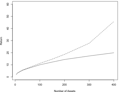
always larger than its theoretical value whenn and pare large and the ratio of the dimension to sample size p/n is not small. They call this problem “over-prediction.” Readers may also refer to Figure 1 for how severe the “over-prediction” is when pandnare large. We note that althoughxis a good estimate ofµand ˆcpis close toc(see Section 5 for the findings),bRp= cˆpx
is not a good estimate ofcµ. This is because in the expression of ˆcp, the eigenvalues ofS are
working on the pentries of a vector with x. So, when we compare them one by one and use the norm of the two-vector difference, it is not very big. But when we compute the return, we actually sum the inverse of the eigenvalues ofS. So it is natural to get an ˆRpthat is much larger
Figure 1: Empirical and theoretical optimal returns for different numbers of assets
0 100 200 300 400
0
10
20
30
40
50
60
Number of Assets
Return
Solid line—the theoretical optimal return (R); Dashed line—the plug-in return (bRp).
In this paper we establish the following theorem to explain the “over-prediction” phenomenon
by analyzing the limiting behaviors ofxTS−1
n x,1TS−n1x, and1TS−n11:
Theorem 4.1. Suppose that
a. Yp = (y1,· · · ,yn) = (yi,j)p,n in which yi,j (i = 1,· · · ,p, j = 1,· · · ,n) are i.i.d. random
variables with Eyi j = 0, E|yi j|2 = 1, E|yi j|4 < ∞, and xk = Σ1/2p yk for each n and for
k= 1,2,· · · ,n;
b. Σp = UpΛpU∗p is nonrandom Hermitian and nonnegative definite with its spectral norm
bounded in p where
Λp =diag( λ|1,· · · , λ1
{z }
, λ|2,· · · , λ2
{z }
, · · · , λ|L,· · · , λL {z }
),
p1, p2, · · · , pL
λ1 > λ2 >· · · > λL, and Up= (Up1,Up2,· · · ,UpL); and
c. for any ap,bp ∈ Cp = {x ∈ Cp}, limp→∞np = y ∈ (0,∞), and aTpUpiU
T
pibp = di, i =
1,2,· · · ,L.
Then, as p,n→ ∞, we have
apTS−n1bp −→
1 (1−y)ap
TΣ−1 bp
where Sn = 1nΣ1/2XpXTpΣ1/2.
Theorem 4.2. Under the conditions stated in Theorem 4.1, as p,n → ∞and p/n → y, the plug-in returnbRp =cˆTpxcould be expressed as:
b
Rp
b
R(1)p = √
µTΣ−1µ
1−y if
1 1−y
σ01TΣ−1µ
√
µTΣ−1µ <1 (Condition 1),
b
R(2)p = 1TΣ−1µ
1TΣ−11 +b˜
(
µTΣ−1µ
− 11TTΣΣ−−11µ11
TΣ−1µ) if 1
1−y
σ01TΣ−1µ
√
µTΣ−1µ >1 (Condition 2),
whereγ= 1/(1−y)and
˜
b=
√
1TΣ−11σ2 0−
√
1−y
µTΣ−1µ1TΣ−11−(1TΣ−1µ)2 .
ObviouslyRbp > Rwhenn,p → ∞and p/n→y∈(0,1). However, whenyis close to zero, b
Rpis close to the theoretical optimal return. This property is illustrated by Table 5 and Figure 1.
There are two problems for the plug-in estimation: one problem is that the conditions ofRbpare
not the same as those of the theoretical return. Obviously,Condition 1in Theorem 4.1 implies that the condition in (2.2) andCondition 2in Theorem 4.1 include two situations: the first one is that 1−y < σ0√1TΣ−1µ
µTΣ−1µ < 1 belongs to the condition in (2.2), and
σ01TΣ−1µ
√
µTΣ−1µ > 1 belongs to the
condition in (2.5). This means that the plug-in estimation may select bR(1)p as the return when
(2.5) is correct. The other problem is thatbR(1)p is √γ times bigger than the real optimal return,
whileRb(2)p is bigger than but may not be √γ times bigger than the theoretical optimal return.
4.2
Bootstrap-Corrected Estimation
To circumvent this limitation, Bai, Liu, and Wong (2009, 2009a) propose a bootstrap technique
to circumvent the limitation of the “plug-in” estimators. They use the parametric approach of
the bootstrap methodology to avoid possible singularity of the covariance matrix estimation in
the bootstrap sample. We describe the details of this procedure as follows: First, a resampleχ∗=
{x∗1,· · · ,x∗n}is drawn from the p-variate normal distribution with meanxand covariance matrix
S defined in equation (3.1). Then, invoking Markowitz’s optimization procedure again on the resampleχ∗, we obtain the “bootstrapped plug-in allocation,” ˆc∗
p, and the “bootstrapped plug-in
return,” ˆR∗p = cˆ∗T
p x∗, where x∗ = ∑n
1x∗k/n. Before we carry on the discussion, we first state
the following proposition, which is one of the basic theoretical foundations for Markowitz’s
optimization estimation:
Proposition 4.1. Assume thaty1,· · · ,ynare n independent random p-vectors of i.i.d. entries
with zero mean and identity variance. Suppose thatxk = µ+zk withzk = Σ
1
entries ofyk’s have finite fourth moments and as p,n→ ∞and p/n→y∈(0,1), we have
µTΣ−1µ
n −→a1 ,
1TΣ−11
n −→a2 , and
1TΣ−1
µ
n −→a3,
satisfying a1a2−a23 >0. Then, with probability 1, we have
lim n→∞ b Rp √ n =
√γa
1> lim
n→∞
R(1)
√
n =
√
a1 when a3 <0,
σ0
√
γ(a1a2−a23)
a2 > nlim→∞ R(2)
√
n =σ0
√
a1a2−a23 a2
when a3> 0,
where R(1) and R(2) are the returns for the two cases given in Proposition 2.1, respectively,
γ =∫b
a
1
xdFy(x)=
1
1−y >1,a= (1−
√y)2, and b =(1+ √y)2.
Applying this proposition, one could conclude that whennis large enough, one could obtain
b
Rp ≃ √γR. We note that the relationAn ≃ Bnmeans that An/Bn → 1 in the limiting procedure
and we say that An and Bn are proportionally similar to each other in the sequel. If Bn is
a sequence of parameters, we shall say that An is proportionally consistent with Bn. As the
relationshipbR∗p ≃ √γbRpis its dual conclusion, one could then obtain the following equation:
√γ(
R−bRp)≃Rbp−bR∗p. (4.2)
Applying the bootstrap-corrected approach to equation (4.2), we could construct the
esti-mate
b
Rb =bRp+
1
√γ(bRp−bR∗p) (4.3)
of the optimal return. In addition, rewriting (4.2), we get
√γ(
cTµ−cˆTx)≃ cˆTpx−cˆ∗pTx∗
and obtain the estimate
ˆ
cb =cˆp+
1
√γ(ˆcp−cˆ∗p) (4.4)
of the corresponding allocation. For simplicity, we callRbb the “bootstrap-corrected return”
and ˆcb the “bootstrap-corrected allocation.”
The main advantage of the bootstrap-corrected estimation is that its return estimate is
consis-tent with the optimal return, and thus, it circumvents the over-prediction problem of the plug-in
return estimate. Hence, one may believe that the bootstrap-corrected estimation is the best
esti-mation for the MV portfolio optimization. Nonetheless, to check how good an estimate of MV
is, but also about how good the estimation of the corresponding allocation is and how big their
risk is.1 According to our simulation in Section 5, we find that the bootstrap-corrected estima-tion does not even outperform the plug-in estimaestima-tion in both allocaestima-tion and risk and sometimes
it could be even worse. We call the former the “allocation estimation” problem and the latter
the “risk” problem. Moreover, our simulation, we find that, yes, the bootstrap-corrected
estima-tion does overcome the “over-predicestima-tion” problem but it incurs an “under-predicestima-tion” problem.
The “under-prediction” is not too serious when the dimension to sample size ratio (y = p/n) is not large but it becomes very serious when y is large. Thus, the bootstrap-corrected esti-mation is not the best MV portfolio optimization. Thus, looking for the best MV portfolio
optimization estimation that could solve all of the defects in the MV portfolio optimization –
the “over-prediction,” “under-prediction,” “allocation estimation,” and “risk” problems – is still
a very important outstanding problem. It is our objective in this paper to obtain an estimation that circumvents all four defects.
4.3
Spectral-Corrected Estimators
In this section, we will first discuss how to estimate the eigenvalues of the population covariance
matrix, and thereafter, we will develop the theory of the spectral-corrected estimators, which
will circumvent all the four defects—the over-prediction phenomenon, the under-prediction
problem, the allocation estimation problem, and the problem of big risk. We will discuss the
details in the following subsections.
4.3.1 Estimation of the eigenvalues of the population covariance and the population co-variance matrix
Letting (sj)1≤j≤p be the peigenvalues of the population covariance matrix Σ, we consider the
spectral distribution (S.D.)HofΣsuch that
H(x)= 1
p
p ∑
j=1
δsj(x), (4.5)
in whichδbis the Dirac point measure atb. It is obvious that the estimation of the eigenvalues
ofΣcould be converted to the estimation of the S.D. ofH as shown in (4.5).
Bai, Chen, and Yao (2010) provide a method to estimate the S.D. of H, when the popu-lation spectrum is of finite support. They prove that their proposed estimate is consistent and
asymptotically Gaussian when the sizekof the limiting support is fixed and known. In addition, when the orderkof the model is unknown, they incorporate a cross-validation procedure in their estimation method to select the unknown model dimension. They also construct the moment
1
relationship between the limits of ESD and the population spectral distribution (PSD), and
then develop the moment estimation. In addition, by using the equations of the limiting spectral distribution of the sample covariance matrix and by adopting the Stietjes transform tools, Li,
Chen, Qin, Yao, Bai (2013) develop a series of new techniques to provide consistent estimation
for the population spectrum distribution. We state the steps to estimate H, the eigenvalues of the population covariance matrix, as follows:
Step 1: SetB= 1nXXT;
Step 2: compute eigenvalues of matrixB, denoted asλ1 ≤λ2 ≤ · · · ≤λp;
Step 3: putBin formula (3.6) to obtain
m(u)=−1−y
u +y
∫ 1
x−udF
B(x),
∀u∈A≡ (−∞, λ1)∪(λp,+∞)\ {0};
Step 4: given{u1,u2,· · · ,uI} ⊂ A, we get{m1,· · · ,mI}={m(u1),· · · ,m(uI)}; and
Step 5: computeHbsuch that
b
H =arg min
H I ∑
i=1
(
u(mi,H)−ui )2
. (4.6)
Then, the S.D.HofΣcan be estimated byHbas shown in (4.6).
From the estimation of the S.D.H ofΣin the above steps, we obtain the eigenvalue estima-tors ˆa1 ≥aˆ2 ≥ · · · ≥aˆp. According to the spectral theory, we have
S =VeΛVT, (4.7)
where Λ =e diag( ˜λ1,· · · ,λ˜p) with ˜λ1 ≥ λ˜2 ≥ · · · ≥ λ˜p and the column vectors of V are the
orthogonal eigenvectors ofS with respect to ˜λ1,· · · ,λ˜p. Suppose thatΛ =b diag{a1ˆ ,a2ˆ ,· · · ,aˆp}
in which ˆa1 ≥ aˆ2 ≥ · · · ≥ aˆp are the estimations of the eigenvalues for matrixΣ; we putbΛin
equation (4.7) and obtain thespectral-corrected covariance
bΣs= VbΛVT. (4.8)
The spectral-corrected covariance in (4.8) could be used in the development of the “best”
4.3.2 Estimation of the optimal return and allocation
After estimating the spectral-corrected covariancebΣsfrom (4.8) and from the steps discussed in Section 4.3.1, one could plug the sample mean vector xand the spectral-corrected covariance
bΣsinto the formulae of the asset allocationcin Proposition 2.1 to obtain
ˆ cs=
σ0bΣ−1
s x
√
xTbΣ−1
s x
if σ0√1TbΣ−s1x
xTbΣ−1
s x
<1,
b
Σ−s11 1TbΣ−1
s 1
+bˆs (
bΣ−s1x− 1TbΣ−s1x
1TbΣ−1
s 1
bΣ−s11
)
if σ0√1TbΣ−s1x
xTbΣ−1
s x
>1, (4.9)
where
ˆ
bs = v t
1TbΣ−1
s 1σ20−1
xTbΣ−1
s x1TbΣ−s11−(1TbΣ−s1x)2
.
Since the estimatorbΣs is obtained by estimating the eigenvalues of the population covariance, we call ˆcsthespectral-corrected allocation. The corresponding return can be estimated by
ˆ
Rs=cˆTsx
which we call thespectral-corrected return. It can also be expressed as
b
Rs= σ0 √
xTbΣ−1
s x if
σ01TbΣ−1
s x
√
xTbΣ−s1x
< 1,
x′bΣ−1
s 1
1TbΣ−1
s 1
+bˆs (
x′bΣ−1
s x−
(
1TbΣ−s1x)2 1TbΣ−1
s 1
)
if σ0√1TbΣ−s1x
xTbΣ−1
s x
> 1.
(4.10)
In addition, the risk of the spectral-corrected allocation can be defined as
Riskcs =cˆTsΣcˆs
= σ2 0x′bΣ−
1
s ΣbΣ−s1x
xTbΣ−1
s x
if σ0√1TbΣ−s1x
xTbΣ−s1x
< 1,
[
AT +bˆs(BT+CT)]Σ[A+bˆs(B+C)] if σ0√1TbΣ−s1x
xTbΣ−1
s x
> 1, (4.11)
which we callspectral-corrected risk. HereA= bΣ−s11
1TbΣ−1
s 1
,B=bΣ−1
s xandC=
1TbΣ−1
s x
1TbΣ−1
s 1
bΣ−1
s 1.
4.3.3 The limiting behavior of the spectral-corrected return
In the previous two subsections, we developed the theory for the construction of the
spectral-corrected estimation. Now, we turn to comparing the performance of the spectral-spectral-corrected
esti-mation with that of the plug-in and bootstrap-corrected estiesti-mations. Does the spectral-corrected
return get closer to the theoretical optimal return? Does the spectral-corrected allocation also get
by an acceptable level? In this subsection and the next subsection we will explore the answers
of the above questions.
We start our discussion with ˆRs. From equation (4.10), we know that x′bΣ−s1x, 1′bΣ−s1x, and
1′bΣ−1
s 1are the main components in the formula of the spectral-corrected return. Thus, we only
need to study the limit of apTbΣ−s1bp that enables us to get the limits of the above-mentioned
items under some regularity conditions. This is because both ap and bp could be x/∥x∥ and
1/√p, and thus, studying the limit ofapTbΣ−s1bp is as good as studying the limits of x
′
∥x∥bΣ−
1
s x
∥x∥, 1′
√pbΣ−1
s x′
∥x∥, and 1′
√pbΣ−1
s 1′
√p. To do so, we first establish the following theorem:
Theorem 4.3. If
a. Yp = (y1,· · · ,yn) = (yi,j)p,n in which yi,j (i = 1,· · · ,p, j = 1,· · · ,n) are i.i.d. random
variables with Eyi j = 0, E|yi j|2 = 1, E|yi j|4 < ∞, and xk = Σ1/2p yk for each n and for
k= 1,· · · ,n;
b. Σp = UpΛpUTp is nonrandom Hermitian and nonnegative definite with its spectral norm
bounded in p where
Λp =diag( λ| 1,· · ·{z , λ}1, λ| 2,· · ·{z }, λ2, · · · , λ| {z }L,· · · , λL ),
p1, p2, · · · , pL
(4.12)
λ1 > λ2 >· · · > λL, Up =(Up1,Up2,· · · ,UpL), andlimpi→∞
pi
n = yi ∈(0,∞); and
c. for the sample covariance matrix Sn =VpeΛVTp expressed in the form as shown in equation
(3.1), the limiting spectral distribution is spectral separated,
then, for any pair of vector sequences{ap},{bp} ∈Cpsatisfying aTpUpiU
T
pibp= di(i= 1,2,· · · ,L),
we have
apTB−p1bp −→ L ∑
k=1 dk
λk L ∑
j=1
λk(uj−λj)
λj(uj−λk)
ςap,bp a.s.,
as p,n→ ∞ and p/n→ y, where Bp = VpΛpVTp, uj is the solution of1+y ∫ t
u−tdH(t)= 0for
any j=1,· · · ,L withλ1> u1> λ2 >· · · > λL> uL> 0.
Applying both Theorem 4.3 and the consistent properties of the spectral estimation (Li,
Chen, Qin, Yao, Bai (2013)), we obtain the following theorem:
Theorem 4.4. Under the conditions stated in Theorem 4.3, as n,p → ∞ and p/n → y, we have
apTbΣ−s1bp −→ L ∑
k=1 dk
λk
L ∑
j=1
λk(uj−λj)
λj(uj−λk)
ςap,bp a.s. (4.13)
We note that ςap,bp is a function of di, λi, and ui (i = 1,· · · ,L) in which di, λi, and ui
(i= 1,· · · ,L) are given in the conditions of Theorem 4.3. Forςap,bp, it is interesting to find the
following result:
apTΣ−1bp<ςap,bp <
ap
TΣ−1b
p
1−y
(4.14)
for any pair of unit vectors ap andbp, in which
apTΣ−1bp
1−y is the limit ofap TS−1
n bp as p,n → ∞
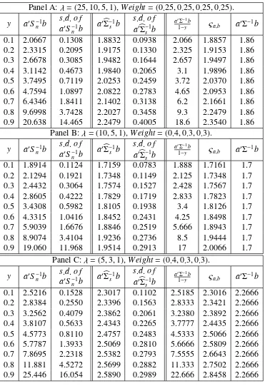
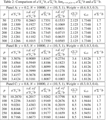
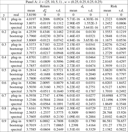
and p/n → y according to Theorem 4.1. In this paper we will evaluate the performance of the spectral-corrected method by simulation and exhibit the simulation results in Tables 1 and
2. These tables report the values of apTS−n1bp, apTbΣ−s1bp, andapTΣ−1bp for a pair of random
bounded vectorsapandbp. From these tables, we notice that
apTΣ−1bp<apTbΣ−s1bp< apTS−n1bp. (4.15)
We also note that the limits of the middle and right terms in equation (4.14) are the
corre-sponding terms in equation (4.15), becauseapTbΣ−s1bp→ |ςap,bp|andap
TS−1
n bp → |
apTΣ−1bp|
(1−y) as p,n→ ∞andp/n→ y.
When we compare the standard deviations (s.d.’s) of the terms in (4.14), we find that
apTbΣ−s1bp is much stabler than apTS−n1bp for any y. When y increases from 0.1 to 0.9, the
performance of bothapTbΣ−s1bp andapTSn−1bp gets worse, but the performance ofapTbΣ−s1bp
im-proves greatly by comparison withapTS−n1bp, not only because the mean of the former is closer
to the theoretical value, but also the s.d. of the former is smaller and the estimation is more
sta-ble than that ofS. In addition, our simulation shows that the inequalities in (4.14) hold. Thus, we recommend that academics and practitioners use the spectral-corrected estimation in their
analysis. To obtain further analysis, we first establish the following theorem:
Theorem 4.5. Under the conditions stated in Theorem 4.3, if
( 1
√p, √1p
)
,
( 1
√p,∥µµ∥
)
, and( µ
∥µ∥,
µ
∥µ∥
)
belong to
{
(υ1, υ2) :υT
1UpiU
T
piυ2 =di ∈R,i= 1,· · · ,L,max{∥υ1∥,∥υ2∥} ≤ M(>0)
}
,
σ0 =ξσ0/√p,∥µ∥/√p=ξµ+o(1), then, as p,n→ ∞and p/n→y, we have
a.
1′bΣ−1
s 1
p −→ς1,1,
1′bΣ−1
s µ
√p
∥µ∥ −→ς1,µ , and
µ′bΣ−1
s µ
∥µ∥2 −→ςµ,µ, (4.16)
b.
1′bΣ−s1x √p
∥x∥ −→ς1,µ and
x′bΣ−s1x
∥x∥2 −→ ςµ,µ, (4.17)
Now, we turn to analyzing the limit of the spectral-corrected return bRs defined in (4.10).
Supposeσ0 = ξσ0/√p. As p,n → ∞ and p/n → y, we first obtain the limit of the condition
stated in (4.10) as follows:
σ01TbΣ−s1x
√
xTbΣ−1
s x
=
ξσ0 1
T
√pbΣ−s1∥xx∥
√ xT
∥x∥bΣ−s1 xT
∥x∥
−→ξσ0
ς1,µ
ςµ,µ .
For the spectral-corrected return stated in (4.10), the first value of bRs possesses the following
limit property:
σ0
√
xTbΣ−1
s x=ξσ0
√
xTbΣ−1
s x
∥x∥2 ·
∥x∥2
p −→ ξσ0ξµ
√ς
µ,µ as p,n→ ∞andp/n→y.
The second value ofbRsin (4.10) becomes
b
Rs =
xTbΣ−1
s 1
1TbΣ−1
s 1
+bˆs x
Tb
Σ−s1x−
(
1TbΣ−1
s x
)2
1TbΣ−1
s 1
= ∥√x∥
p
xT
∥x∥bΣ−
1
s 1
√p
1
√pTbΣ−1
s √1p
+bˆs∥x∥2 xT ∥x∥bΣ
−1
s
x ∥x∥−
( 1
√pTbΣ−s1 x
∥x∥
)2
1
√pTbΣ−1
s √1p .
Here, as p,n→ ∞and p/n→y, we have
ˆ
bs∥x∥2 = ∥x∥2 v t
1TbΣ−1
s 1σ20−1
xTbΣ−1
s x1TbΣ−s11−(1TbΣ−s1x)2
= ∥√x∥
p v u u u t 1
√pTbΣ−1
s √1pξσ0 −1 x
∥x∥ T
bΣ−1
s x
∥x∥ 1
√pTbΣ−1
s 1
√p −(√1pTbΣ−1
s x
∥x∥)2
−→ ξµ
√
ς1,1ξσ0 −1
ςµ,µς1,1−(ς1,µ)2
.
Thus, as p,n→ ∞and p/n→y, we obtain
b
Rs−→ ξµ
ς1,µ
ς1,1
+ξµ
√
ς1,1ξσ0 −1
ςµ,µς1,1−(ς1,µ)2
(
ςµ,µ−
(ς1,µ)2
ς1,1 )
. (4.18)
According to the above analysis, we obtain the following theorem:
Theorem 4.6. Under the conditions and definitions stated in Theorem 4.5, as n,p→ ∞and p/n→y, we have
b
Rs−→
ξσ0ξµ√ςµ,µ if ξσ0ς1,µ/ςµ,µ <1,
ξµ ς1,µ
ς1,1 +ξµ
√ ς
1,1ξσ0−1
ςµ,µς1,1−(ς1,µ)2
(
ςµ,µ− (ς1,µ)2
ς1,1
)
In this paper we hypothesize the conjecture that Rbs is proportionally consistent with the
theoretical optimal return R defined in (2.3) or (2.6) under some regularity conditions. The results in Theorem 4.6 help us to check this conjecture. To complete the work, we establish the
limit of the theoretical optimal return as shown in the following theorem:
Theorem 4.7. Under the conditions of Theorem 4.5, as p,n→ ∞and p/n→ y, we have
a. the limits of
1′Σ−11
p ,
1′Σ−1µ √p
∥µ∥ , and
µ′Σ−1µ
∥µ∥2 exist, and
b. the theoretical optimal return R satisfies
R−→
ξσ0ξµ
√
ς0
µ,µ if ξσ0ς01,µ/ςµ,µ0 <1,
ξµ ς0
1,µ
ς0
1,1
+ξµ
√
ς0
1,1ξσ0−1 ς0
µ,µς10,1−(ς1,µ)2
(
ς0 µ,µ−
(ς0
1,µ)2
ς0
1,1
)
if ξσ0ς01,µ/ςµ,µ0 >1,
whereς0
1,1,ς
0
1,µ, andςµ,µ0 are the corresponding limits in (a).
From Table 1, we find that (ς1,1, ς1,µ, ςµ,µ) is very close to (ς10,1, ς10,µ, ςµ,µ0 ). Thus, Theorems
4.6 and 4.7 and our simulation results support the conjecture thatbRsisproportionally consistent
with the theoretical optimal returnRunder some regularity conditions.
4.3.4 The limiting behavior of the spectral-corrected risk
In this paper, we also hypothesize the conjecture that the spectral-corrected riskRiskcs (defined in equation (4.11)) is close to theRisk of the theoretical optimal return under some regularity conditions. To examine this conjecture, in this section we will study the limiting behavior of the spectral-corrected risk. To do so, from (4.11), we only need to examine the limiting behavior of
apTbΣ−s1ΣbΣ−s1bpas stated in the following theorem:
Theorem 4.8. Suppose that the projections on each Uj (j = 1,· · · ,L)subspace of vectors ap
and bp only have finite nonzero entries. Then, under the same conditions of Theorem 4.3, we
have
apTB−p1ΣB−
1
p bp−→
L ∑
k=1 dk λk L ∑
j=1
λk(uj−λj)
λj(uj−λk)
2
ϱap,bp a.s. (4.19)
From Theorem 4.8, we notice that ϱap,bp depends only on the information of dk, λk, and
uk (k = 1,· · · ,L) about the population. Since it is difficult to obtain the theoretical result for
bounded vectorap,bp, in this paper we conduct a simulation for the comparison and report the
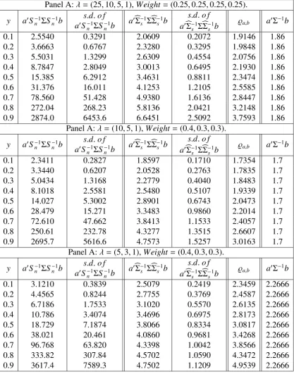
results in Tables 3 and 4. Table 3 shows that, compared withapTS−n1ΣSn−1bpandapTbΣ−s1ΣbΣ−s1bp,
the limit ofapTbΣ−s1ΣbΣ−s1bpis much closer to the real valueapTΣ−1bpfor anyy. From the results
in Table 4, one could easily observe that apTbΣ−s1ΣbΣ−s1bp converges. Thus, we establish the
following theorem for the spectral-corrected riskRisks c:
Theorem 4.9. Under the conditions of Theorem 4.5, if p,n→ ∞and p/n→ y, then
a. the limits of
1TbΣ−1
s ΣbΣ−s11
p ,
1TbΣ−1
s ΣbΣ−s1µ
√p
∥µ∥ , and
µTbΣ−1
s ΣbΣ−s1µ
∥µ∥2 , exist and they are denoted byϱ1,1,ϱ1,µ andϱµ,µ, and
b.
1TbΣ−1
s ΣbΣ−s11
p −→ϱ1,1,
1TbΣ−1
s ΣbΣ−s1X
√p
∥X∥ −→ ϱ1,µ,
XTbΣ−s1ΣbΣ−s1X
∥X∥2 −→ϱµ,µ.
In addition, we have
c. whenξσ0ς1,µ/ςµ,µ <1,
p·Riskcs→ ξσ0ϱµ,µ ςµ,µ
a.s., and
d. whenξσ0ς1,µ/ςµ,µ >1, p·Riskcsalmost surely converges to
ϱ1,1
ς1,1
+ ϱ1,1
ξµς1,1 √
ς1,1ξσ0 −1
ςµ,µς1,1−(ς1,µ)2
+
√
ς1,1ξσ0 −1
ςµ,µς1,1−(ς1,µ)2
ϱµ,µ−2
ς1,µϱ1,µ ς1,1
+
(ς 1,µ
ς1,1 )2
ϱ1,1 .
We note that in Theorem 4.9, if we suppose thatσ0 = ξσ0
√p, then we have p·Risk → ξσ0 as p,n→ ∞and p/n → y. We also note that the limit of p·Riskcsis not equal to that of p·Risk. However, it is closer to that of p·Riskthan the other two risks.
In addition, from Table 4, we observe that (ϱ1,1, ϱ1,µ, ϱµ,µ) is very close to (ς10,1, ς10,µ, ςµ,µ0 ).
Thus, Risks
c is close to the theoretical risk. Theorems 4.6, 4.7, and 4.9 and our simulation
results support our conjecture that Riskcs is close to theRisk of the theoretical optimal return under some regularity conditions.
5
Simulation Study
In this section, we will conduct simulation to compare (1) how good the performance of the
spectral-corrected returnbRsis in comparison with that of the plug-in returnRbp and
comparison with that of the plug-in allocation ˆcpand bootstrap-corrected allocation ˆcb, and (3)
what the risks of the plug-in return bRp, bootstrap-corrected return bRb, and spectral-corrected
returnRbs, and among them, which one is smallest.
In order to check how good the performance of the spectral-corrected return bRs is in
com-parison with that of the plug-in returnRbp and bootstrap-corrected returnbRb, we define
dRω =Rω−R with ω = p,b,s (5.1)
in which we call dRs the spectral-corrected difference for the return, which is the difference between the spectral-corrected optimal return estimate ˆRs and the theoretic optimal return R.
The plug-in difference dRp and bootstrap-corrected difference dbR for the return are defined similarly as stated in (5.1).
To check how good the performance of the spectral-corrected allocation ˆcsis in comparison
with that of the plug-in allocation ˆcpand bootstrap-corrected allocation ˆcb, we define
dcω =∥cˆω−c∥ with ω = p,b,s (5.2)
in which we call dcs the spectral-corrected normed difference for the allocation, which is the normed difference between the spectral-corrected optimal allocation estimate ˆcs and the
theoretic optimal allocationc. Theplug-in normed differencedcpand thebootstrap-corrected
normed differencedb
c are defined similarly as stated in (5.2).
Among the risks of the plug-in returnRbp, bootstrap-corrected return, and spectral-corrected
returnRbs, to check which one is the smallest, we define
Riskωc = cˆ′ωΣcˆω, with ω = p,b,s (5.3)
in which we call Riskcb, Riskcp, and Riskcs the plug-in risk, bootstrap-corrected risk, and
spectral-corrected risk, respectively. We will also compare dωc, dωR, and riskωc for ω = p,b,s
with those for the theoretical optimal returnR. They aredR R,d
c
c, andRiskcc such that
dRR = R−R=0 , dcc = ∥c−c∥= 0 , and Riskcc =c′Σc= 1. (5.4)
Given a p-dimension nonzero vectorµ = (µ1,· · · , µp)T and a positive definite matrix Σ =
(σi j), which is assumed to be a diagonal matrix for simplicity, we state the simulation procedure
as follows:
Step 1: For each round of N times simulation, we will first fix p and choose µ = (µ1,· · · , µp)T
in which each µi is generated from U(−1,1). We will then select λ = (λ1, ..., λp), and
Weight = (p1
p, ..., pL
p )
. Thereafter, we set Σ = Λp in which Λp is defined in equation (4.12).2 We will fix p,µ, andλfor each round of simulation.
2