A Conditional Value at Risk Based Portfolio Selection With Dynamic Tail Dependence Clustering

Munich Personal RePEc Archive

A Conditional Value-at-Risk Based

Portfolio Selection With Dynamic Tail

Dependence Clustering

De Luca, Giovanni and Zuccolotto, Paola

University of Naples Parthenope, University of Brescia

August 2013

A Conditional Value-at-Risk Based Portfolio Selection

With Dynamic Tail Dependence Clustering

Abstract

In this paper we propose a portfolio selection procedure specifically

designed to protect investments during financial crisis periods. To this

aim, we focus attention on the lower tails of the returns distributions

and use a combination of statistical tools able to take into account the

joint behavior of stocks in event of high losses. In detail, we propose to

firstly cluster time series of stock returns on the basis of their lower tail

dependence coefficients, estimated with copula functions, and secondly to

use the obtained clustering solution to build an optimal minimum CVaR

portfolio. In addition, the procedure is defined in a time-varying context,

in order to model the possible contagion between stocks when volatility

increases. This results in a dynamic portfolio selection procedure, which

is shown to be able to outperform classical strategies.

Keywords: Copula functions, Tail dependence, Time series clustering.

1

Introduction

In the multivariate analysis of financial returns, the association between

ex-tremely negative values has recently become a hot topic of research due to the

recent financial crisis.

Basic portfolio theory suggests that it is not desirable to hold in portfolio

simultane-ous drop of them could generate a considerable reduction of the value of the

portfolio. However, a more refined analysis might reveal that a measure of the

total association between the returns of two assets does not always provide a

measure of the actual association between the lowest returns of the same assets.

This implies that some popular measures of association, such as the correlation

coefficient, the Kendall’s tau and so on, do not always ensure the desired

de-gree of diversification of a portfolio. On the other hand, an effective measure

of the relationship between extremely low returns of two assets is the lower tail

dependence because it is built taking into account the behavior of the lower tail

returns, and ignoring both the central returns and the upper tail returns.

Moreover, the selection of assets with a low association between extremely

low returns to compose a portfolio could be made difficult by the high number

of assets available on the market.

In order to find an efficient way for selecting assets to form a portfolio keeping

as low as possible the association between extreme negative returns, De Luca

and Zuccolotto (2011, 2012) have proposed a multi-step procedure consisting of

four steps:

(a) the estimation of the lower tail dependence coefficients of all the possible

pairs of assets;

(b) the clustering of the assets according to the coefficients into groups

char-acterized by high lower tail association;

(d) the choice among all the possible portfolios according to a specified

crite-rion.

In this paper, in order to take into account our focus on extreme events the

choice among all the possible portfolios composed of assets belonging to

differ-ent clusters is made minimizing the Conditional Value-at-Risk (Rockafellar and

Uryasev, 1997) rather than the variance or other dispersion measures. Moreover,

we follow the idea that the lower tail dependence is not time-invariant, but has

its own dynamics. As a result, the clustering of the assets is time-varying, and

the possible portfolios one can compose also change over time. This approach is

motivated by the recurring and erratic movements of the financial markets that

can dramatically shed light on the limitations of the traditional static analyses.

The paper is organized as follows. In Section 2 the definition of lower tail

dependence is given and a conveniently flexible time-varying copula model is

proposed. Section 3 presents a clustering procedure based on the estimated

lower tail dependence coefficients in a dynamic context, while Section 4 explains

how to exploit it to compose a portfolio. In Section 5 a case study allows the

comparison of two strategies of portfolio selection, named A and B. Strategy A

is based on a stable clustering solution obtained summarizing all the solutions

obtained at the T times of observations. Strategy B uses at each time the

one-step-ahead forecast of the dissimilarity matrix to determine the clustering

solution, so it is inherently dynamic. A comparison with other portfolio selection

rules, such as the Markowitz mean-variance model, is discussed. Finally, Section

2

Dynamic tail dependence coefficients

The tail dependence is a measure of association between extremely low or high

values. Let us provide some details in the bivariate case. Given two variables,

Y1 and Y2 and their respective distribution functions F1(Y1) and F2(Y2), the

lower tail dependence coefficient is defined as

λL= lim

u→0+P(F1(Y1)< u|F2(Y2)< u)

that is the probability thatY1 assumes an extremely low value, given that an

extremely low value has already occurred toY2.

On the other hand, if the interest is focused on very high values, the upper

tail dependence coefficient is defined as

λU = lim

u→1−

P(F1(Y1)≥u|F2(Y2)≥u)

that is the probability thatY1 assumes an extremely high value, given that an

extremely high value has occurred toY2.

In a parametric approach these probabilities are model-dependent, that is

the choice of a model for the bivariate set of data implies or neglects non-null

tail dependence coefficients. A bivariate Gaussian model is a typical example

of model which does not admit any tail dependence. Therefore, this parametric

hypothesis is valid only if the assumption of no association between extreme

values is reasonable.

In the analysis of bivariate financial returns, the inadequacy of the Gaussian

paradigm is widely acknowledged. The tails of the empirical univariate

empirical bivariate distributions show an association among extreme values not

encountered in the bivariate Gaussian distribution.

A more complex but flexible way of describing a set of bivariate data is the

use of a copula function. A bivariate copula function is defined as a function

C : [0,1]2 _{→ [0,1] such that the joint distribution function F(y}

1, y2) can be

written as

F(y1, y2) =C(F1(y1), F2(y2))

for ally1,y2(see Nelsen, 2006).

The flexibility of the copula functionC allows us to model the joint density

separating the marginal distributions from the dependence structure.

In this case, it is easy to show that the tail dependence coefficients can be

written in terms of the copula function. In particular, the lower tail dependence

coefficient is given by

λL= lim

u→0+

C(u, u)

u

while the upper tail dependence coefficient is

λU = lim

u→1−

1−2u+C(u, u)

1−u .

Given the wide variety of copula functions, one can select a function with no

tail dependence, or a function with only one tail dependence (lower or upper)

or a function which admits both tail dependence in a symmetric or asymmetric

way. In the analysis of financial returns, an association between extreme values

is usually detected in both the tails. So, a natural choice is a fairly general

Joe-Clayton copula function (Joe, 1997) meets this basic requirement and is

easily estimable. In the bivariate case, the Joe-Clayton copula function is given

by

C(u1, u2) = 1− {1−[(1−(1−u1)κ)−θ+

(1−(1−u2)κ)−θ−1]−1/θ}1/κ, (1)

where ui represents the distribution function of the i-th variable. The

Joe-Clayton copula depends on two parameter, θ > 0 and κ ≥1. The lower and

upper tail dependence coefficients are determined by, respectively,θandκ, that

is

λL= 2−

1

θ

and

λU = 2−2

1

κ.

A time-invariant copula involves constant tail dependence. However,

finan-cial markets constitute a dynamic context exposed to many different stresses.

As a result the constancy of tail dependence could be a restrictive assumption.

In this work we relax this hypothesis, proposing a time-varying Joe-Clayton

copula function. In particular, as our interest lies in the lower tail, that is in

the relationship between extremely negative returns, we propose a time-varying

model only for the parameterθ, driving the lower tail dependence coefficient,

while κ is kept constant. Moreover, we assume that the dynamics ofθ is

af-fected by the past volatility of the market. In particular, denoted θt and σt,

the time-varying Joe-Clayton copula is given by

C(u1t, u2t) = 1− {1−[(1−(1−u1t)κ)−θt+

(1−(1−u2t)κ)−θt−1]−1/θt}1/κ, (2)

and

∆θt=α(σt−1−γ). (3)

The interpretation ofγ is surely interesting. It can be seen as a threshold.

Whenα >0, if the volatility at timet−1 is over the threshold, then an increase

ofθis expected, that is ∆θt>0. Viceversa, ifσt−1is under the threshold, then

∆θt<0. When the parameterαis negative, an opposite mechanism works.

Equation (3) can be written as

∆θt=ω+ασt−1

whereω=−αγ and finally

θt=ω+θt−1+ασt−1.

Then, the time-varying lower tail dependence coefficient is obtained as

λLt= 2−1/θt. (4)

3

Dynamic time-series clustering

3.1

The clustering procedure

In this paper we refer to the clustering procedure proposed in De Luca and

dissimilarity measure defined as

δ({yit},{yjt}) =δij =−log(ˆλL), (5)

where {yit}t=1,...,T and {yjt}t=1,...,T denote the time series of returns of two

assetsiandj, and ˆλL is their estimated tail dependence coefficient.

Given the time series of the returns ofpassets, the clustering procedure is

composed of two steps. In step 1, starting from the dissimilarity matrix ∆ =

(δij)i,j=1,...,p, anoptimalrepresentation of theptime series{y1t}, . . . ,{ypt}asp

pointsy₁, . . . ,yp in Rq is found by means of Multidimensional Scaling (MDS).

The termoptimalmeans that the Euclidean distance matrixD= (dij)i,j=1,...,p,

with dij =kyi−yjk, of the ppoints y1, . . . ,yp in Rq has to fit as closely as

possible the dissimilarity matrix ∆. The extent to which the interpoint distances

dij “match” the dissimilarities δij is measured by an index calledstress, which

should be as low as possible. The algorithm of MDS works for a given value

of the dimensionq, which has to be given in input. So, it is proposed to start

with the dimensionq= 2 and then to repeat the analysis by increasing quntil

the minimum stress of the corresponding optimal configuration is lower than a

given threshold ¯s. In step 2, theppointsy1, . . . ,yp in Rq are clustered using a

k-means algorithm.

The clusters obtained with this procedure are composed of assets

character-ized by high tail dependence in the lower tail. De Luca and Zuccolotto (2011,

2012) show that the clustering solution obtained with this procedure can be

effectively exploited for portfolio selection. The basic idea consists of avoiding

possible extreme losses. So, we should select assets by imposing the restriction

that each asset belongs to a different cluster. This protects the investments from

parallel extreme losses during crisis periods, because the clustering solution is

characterized by a moderate lower tail dependence between clusters.

3.2

The dynamic clustering procedure

Through the copula function described in Section 2 we obtain time-varying

estimates of the tail dependence coefficients. Given two time series of financial

returns {yit}t=1,...,T and {yjt}t=1,...,T, let ˆλLt be their lower tail dependence

estimate at time t. The dissimilarity measure (5) between the two series can

then be computed for each timetas

δij,t=−log(ˆλLt). (6)

On the whole, given the time series of returns ofpassets, we get time-varying

(p×p) dissimilarity matrices

∆t= (δij,t)i,j=1,...,p;t=1,...,T. (7)

So, we can sequentially apply the clustering procedure described in Section 3.1

to the matrices ∆t,t= 1, . . . , T, thus obtaining a different clustering solution at

each timet. The groups composition is dynamically adapted to the variations

due to the changes in the copula function parameter. The dynamics of the

clustering solutions can be inspected in different ways: the overall discordance

between the clustering at time t−1 and that at time t can be measured by

(Rand, 1971). Alternatively, we could examine the patterns of some pairs of

assets (same cluster/different cluster) we are interested to.

Finally, the dynamic of the whole period can be summarized by computing,

for each pair of assetsij, the index

bij = 1−

PT t=1Iij,t

T (8)

where Iij,t is the indicator function which equals 1 if stock i and stock j are

assigned to the same cluster at timetand 0 otherwise. The indexbij denotes the

fraction of the total clustering solutions with stocksiandjbelonging to different

clusters, a generalization of the widely used Simple Matching distance, due to

Sokal and Michener (1958). So, we can perform a clustering algorithm using the

distance matrixB= (bij)i,j=1,...,p, in order to summarize theT dynamic cluster

solutions. The final clustering solution obtained using the distance matrix B

will be calledOverall Dynamic Clustering(ODC).

4

Portfolio selection

In our idea, the main challenge of clustering is the possibility to use it for

build-ing a portfolio able to protect investments durbuild-ing periods when extreme losses

could occur simultaneously for many stocks, due to contagion phenomenons.

As pointed out in the Introduction, in this paper we improve the method

proposed in De Luca and Zuccolotto (2011, 2012) firstly by using a portfolio

se-lection procedure focused on extreme events, coherently with the tail dependence

over time.

About the first point, we propose to build portfolios by optimizing

Conditional-Value-at-Risk (CVaR), a measure of risk defined by Rockafellar and Uryasev

(2000) as the expected loss exceeding Value-at Risk (VaR) and better fitting

in our context, where the focus is on the tails of the probability distributions.

In the literature, CVaR is also called Mean Excess Loss, Expected Shortfall,

or Tail VaR. LetY = (Y1, . . . , Yp)′ be a multiple random variable with

prob-ability densityf(Y), describing the returns of passets at a given time t, and

w= (w1, . . . , wp)′,w1+. . .+wp= 1, a vector of weights of thepassets in a

port-folioP(Y,w). The loss associated to P(Y,w) is given byL(Y,w) =−w′_Y.

For a given probability level β ∈ (0,1), VaRβ and CVaRβ are defined

respec-tively as

VaRβ= min{α∈R: Ψ(w, α)≥β}

CVaRβ=

Z

L(Y,w)≥VaRβ

L(Y,w)f(Y)dY

(1−β)

where

Ψ(w, α) =

Z

L(Y_,w_)≤α

f(Y)dY.

In order to identify the set of weights w minimizing CVaRβ for a given β,

Rockafellar and Uryasev (2000) define the following objective function

S(w,VaRβ) = VaRβ+

Z

Y∈Rp

[−w′Y−VaRβ]+f(Y)dY

(1−β)

where [a]+ _{= awhen a > 0 and [a]}+ _{= 0 otherwise. Given the time series of}

yt = (y1t, . . . , ypt)′ be the vector of p observations at time t. The objective

functionS(w,VaRβ) can then be approximated using data as

ˆ

S(w,VaRβ) = VaRβ+

T

X

t=1

ut

T(1−β) (9)

whereut= max{−w′yt−VaRβ; 0}. We have to compute the values ofw and

VaRβ that minimize function (9), subject to the following linear constraints:

• w1+. . .+wp= 1;

• w′_{¯y ≥y}

min, where ¯y= T−1PTt=1yt and ymin is the minimum allowed

expected return for the portfolioP(Y,w);

• ut≥0 andw′yt+ VaRβ+ut≥0 for t= 1, . . . , T.

The problem can be solved with linear programming. Further details about

portfolio optimization with minimum CVaR objective can be found in

Rockafel-lar and Uryasev (2000) and Krokhmalet al. (2002).

So, we propose the following two strategies for clustering based portfolio

selection:

1. Use time series of price returns ofpstocks at time 1, . . . , T;

2. fit each time series with a proper univariate model accounting for possible

autocorrelation and heteroskedasticity;

3. using thei.i.d.residuals of the marginal models, estimate the parameters

of all the bivariate time-varying copula functions (a total of 0.5p(p−1)

4. compute theT dissimilarity matrices ∆t= (δij,t)i,j=1,...,p;t=1,...,T

accord-ing to (7).

Strategy A

(5A) Determine the ODC clustering solution descibed above, using the distance

matrixB= (bij)i,j=1,...,p, withbij computed by (8). Letkbe the number

of clusters;

(6A) for a fixedβ, build all the possible Minimum CVaR Portfolios composed by

kstocks not belonging to the same cluster of the ODC clustering solution;

(7A) select the Minimum CVaR Portfolio with the lowest CVaR value.

Strategy B

(5B) At timeT, compute the one-step-ahead forecast of the dissimilarity matrix

∆T+1 and determine the clustering solution for timeT+ 1 using the

two-step procedure described in section 3.1. Letkbe the number of clusters;

(6B) for a fixedβ, build all the possible Minimum CVaR Portfolios composed

by k stocks not belonging to the same cluster of the clustering solution

determined in the previous step;

(7B) select the Minimum CVaR portfolio with the lowest CVaR value.

The fundamental difference between strategy A and B lies in the nature of

the clustering solution employed to determine the composition of the candidate

all the clustering solutions obtained at the T times 1, . . . , T, while strategy B

uses the specific instantaneous clustering solution determined at time T + 1.

Thus, strategy A is based on a stable clustering solution and the corresponding

portfolio does not need to be frequently updated, while strategy B is based on

clustering solutions that can potentially change every day, and frequent revision

is then recommended. The choice between the two strategies depends on the

state of the market: strategy B can be useful during periods with high instability.

5

Case study

In this case study we analyse the time series of the daily price returns of the

p = 24 Italian stocks which have been included in FTSE MIB index during

the whole period from January 3, 2006 to October 31, 2011 (T = 1481). We

firstly estimate the marginal models of the p time series by fitting data with

univariate Student-t AR-GARCH models, in order to take into account the

possible presence of autocorrelation and heteroskedasticity. Then the copula

function is estimated using the distribution functions computed on the i.i.d.

residuals of the marginal models.

5.1

Estimation of dynamic tail dependence coefficients

For each pair of standardized residuals, the time-varying Joe-Clayton copula

function (2) has been estimated using equation (3) for modellingθt.

The copula density has been maximized using a routine written in Gauss

The estimates for the 276 pairs of residuals can be summarized as follows:

(a) the estimates ofωrange from -0.0027 to approximately 0; in 235 cases out

of 276 the estimate is negative;

(b) the estimates of αrange from -0.0756 to 0.2125; in 234 cases out of 276

the estimate is positive;

(c) the estimates of κrange from 1.0387 to 1.8898.

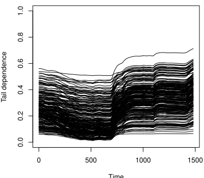
We have then computed the time-varying lower tail dependence coefficients

according to (4). Figure 1 gives a rough summary of the dynamics of the 234

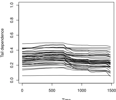
estimated coefficients characterized by a positiveα, while Figure 2 contains the

dynamics of the remaining 42 coefficients with a negativeα.

The analyzed period is characterized by low volatility in the first half, then,

at the end of 2008 a peak in the volatility is observed, followed by an uncertain

period with a swing of volatility. This is reflected in the dynamics of the (lower)

tail dependence. For the pairs with an estimated positiveα(the majority), the

tail dependence is weaker in the first half, grows up rapidly at the end of the

2008, then its increase is slow until the end of the period (October 2011). In

a very few cases, and only for the last part of the period of observation, the

tail dependence coefficient is greater than 0.60. In general, the range of the

coefficients is wide. At the beginning of the sample period (January 2006) the

coefficients approximately range from 0.05 to 0.55, before the crisis from 0.01

to 0.50, at the end (October 2011) from 0.05 to 0.70. For the remaining pairs

0 500 1000 1500

0.0

0.2

0.4

0.6

0.8

1.0

Time

T

ail dependence

Figure 1: Dynamics of the lower tail dependence of the 234 pairs with positive

α.

presents very small changes also in correspondence of the peaks of the volatility.

The coefficients range from 0.05 to 0.50.

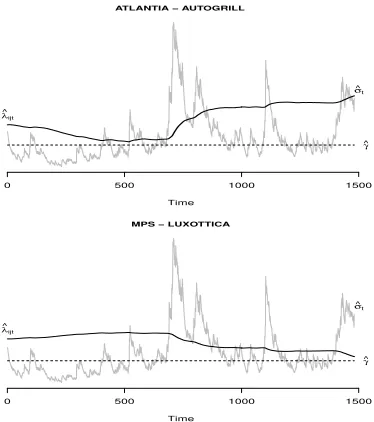
Moreover, we report two cases characterized by a different sign ofα. The

former is the pair ATLANTIA-AUTOGRILL presenting a positiveα, the

lat-ter the pair MPS-LUXOTTICA characlat-terized by a negative sign ofα. Figure

3 depicts the estimated time-varying lower tail dependence coefficients of the

two pairs, ATLANTIA-AUTOGRILL (top) and MPS-LUXOTTICA (bottom),

with the estimated one-lagged volatility of the market superimposed and the

estimated thresholds ˆγ. We can observe that when the volatility is below the

0 500 1000 1500

0.0

0.2

0.4

0.6

0.8

1.0

Time

T

ail dependence

Figure 2: Dynamics of the lower tail dependence of the 42 pairs with negative

0 500 1000 1500

ATLANTIA − AUTOGRILL

Time

γ

^

λ

^ ijt

σ^t

0 500 1000 1500

MPS − LUXOTTICA

Time

γ

^

λ

^ ijt

σ^t

Figure 3: Lower tail dependence coefficient at timet and market volatility at

timet−1 for the pairs ATLANTIA-AUTOGRILL (top) and MPS-LUXOTTICA

0 500 1000 1500

0.0

0.2

0.4

0.6

0.8

1.0

ATLANTIA − AUTOGRILL (tail dependence)

Time

λ

^ijt

0 500 1000 1500

0.0

0.5

1.0

1.5

ATLANTIA − AUTOGRILL (dissimilarity)

Time

δ

^ijt

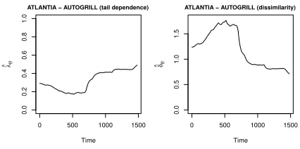
Figure 4: Lower tail dependence coefficient (left) and dissimilarity index (right)

for the pair ATLANTIA-AUTOGRILL.

tends to decrease, on the other hand, when the volatility exceeds the threshold

the same coefficient tends to increase. In particular, in correspondence of the

middle highest peak of the volatility and, in the second part of the sample

pe-riod, of the other two peaks, the coefficient shows more pronounced increases.

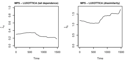
For the pair MPS-LUXOTTICA, the opposite behavior is observed.

Finally, Figure 4 depicts the lower tail dependence coefficient (left) and the

dissimilarity index (right) of the pair ATLANTIA-AUTOGRILL. In Figure 5

the same graphs are reported for the pair MPS-LUXOTTICA.

5.2

Dynamic clustering

After the estimation of the 0.5p(p−1) = 276 bivariate copula functions, the

sequence of the estimated time-varying (p×p) dissimilarity matrices ∆t =

(δij,t)i,j=1,...,p;t=1,...,T is computed as in (7). By sequentially applying the

clus-tering procedure described in Section 3.1 to the matrices ∆t, t = 1, . . . , T, we

0 500 1000 1500

0.0

0.2

0.4

0.6

0.8

1.0

MPS − LUXOTTICA (tail dependence)

Time

λ

^ijt

0 500 1000 1500

0.0

0.5

1.0

1.5

MPS − LUXOTTICA (dissimilarity)

Time

δ

^ijt

Figure 5: Lower tail dependence coefficient (left) and dissimilarity index (right)

for the pair MPS-LUXOTTICA.

Computations are carried out using the R functionsisoMDSfor MDS,kmeans

andcclustfork-means clustering.

From an operative point of view, since the k-means clustering solutions can

be different from one run to another of the algorithm, at each timetthe following

procedure is used for each value of k, k = 1, . . . , K, where K is fixed by the

researcher and denotes the maximum reasonable number of clusters. In this

case study we have fixed the valueK= 10.

Firstlykmeansis executed 8 times with the Hartigan-Wong algorithm

(Har-tigan and Wong, 1979).

Then, the centroids of the solution with the highest ratio of the variance

between over the total variance are used as optimal initial values for cclust

which, in its turn, is executed 3 times and the best solution is chosen according

to the same criterion of the highest ratio of the variance between over the total

variance.

number of clusters is selected as the most voted by the following indices (for

a comprehensive review, see Dimitriadou et al., 2002): RL (Ratkowsky and

Lance, 1978), SS (Scott and Symons, 1971), FR (Friedman and Rubin, 1967),

DB (Davies and Bouldin, 1979), SSI (Dolniˇcaret al., 1999).

For each pair of stocksij, at each timetwe record the valueIij,t = 1 if the

two stock belong to the same cluster andIij,t= 0 otherwise. Figure 6 shows the

scatterplots ofIij,t againstσt−1 fori=Atlantiaand j all the other 23 stocks

(solid lines denote a kernel smoothing showing the basic average patterns).

For low levels of volatility the pattern is sometimes wavering, but when

volatility increases, the pairs tend to be more stably assigned either to the same

or to a different cluster, as a result of the stronger tail dependence characterizing

some pairs of stocks during high volatility periods. Similar graphs are obtained

for the other pairs of stocks. Finally, the ODC clustering solution is determined

by applying a hierarchical algorithm (Ward linkage) to the distance matrix

B= (bij)i,j=1,...,p withbij computed by (8). The obtained cluster dendrogram

is displayed in Figure 7, withk= 5 clusters selected.

5.3

Portfolio selection

In this section we show the results of portfolio selection according to the two

ATLANTIA

0.01 0.03 0.05

0.0 0.2 0.4 0.6 0.8 1.0 AUTOGRILL

0.01 0.03 0.05

0.0 0.2 0.4 0.6 0.8 1.0 MPS

0.01 0.03 0.05

0.0 0.2 0.4 0.6 0.8 1.0 ENEL

0.01 0.03 0.05

0.0 0.2 0.4 0.6 0.8 1.0 ENI

0.01 0.03 0.05

0.0 0.2 0.4 0.6 0.8 1.0 FIAT

0.01 0.03 0.05

0.0 0.2 0.4 0.6 0.8 1.0 FINMECC

0.01 0.03 0.05

0.0 0.2 0.4 0.6 0.8 1.0 FONDIARIA

0.01 0.03 0.05

0.0 0.2 0.4 0.6 0.8 1.0 GENERALI

0.01 0.03 0.05

0.0 0.2 0.4 0.6 0.8 1.0 INTESA

0.01 0.03 0.05

0.0 0.2 0.4 0.6 0.8 1.0 LOTTOMAT

0.01 0.03 0.05

0.0 0.2 0.4 0.6 0.8 1.0 LUXOTTICA

0.01 0.03 0.05

0.0 0.2 0.4 0.6 0.8 1.0 MEDIOBANCA

0.01 0.03 0.05

0.0 0.2 0.4 0.6 0.8 1.0 MEDIOLANUM

0.01 0.03 0.05

0.0 0.2 0.4 0.6 0.8 1.0 MEDIASET

0.01 0.03 0.05

0.0 0.2 0.4 0.6 0.8 1.0 PIRELLI

0.01 0.03 0.05

0.0 0.2 0.4 0.6 0.8 1.0 BPM

0.01 0.03 0.05

0.0 0.2 0.4 0.6 0.8 1.0 SAIPEM

0.01 0.03 0.05

0.0 0.2 0.4 0.6 0.8 1.0 SNAM

0.01 0.03 0.05

0.0 0.2 0.4 0.6 0.8 1.0 STM

0.01 0.03 0.05

0.0 0.2 0.4 0.6 0.8 1.0 TELECOM

0.01 0.03 0.05

0.0 0.2 0.4 0.6 0.8 1.0 TERNA

0.01 0.03 0.05

0.0 0.2 0.4 0.6 0.8 1.0 UBI

0.01 0.03 0.05

0.0 0.2 0.4 0.6 0.8 1.0 UNICREDIT

MEDIOBANCA FONDIARIA UNICREDIT

UBI _{BPM MPS}

INTESA

SAIPEM

STM

A

UT

OGRILL

LUXO

TTICA FIA

T

PIRELLI SNAM TERNA ENEL ENI

MEDIOLANUM GENERALI MEDIASET FINMECC TELECOM ATLANTIA LO

TT

OMA

T

0

1

2

3

4

5

Cluster Dendrogram

Hierarchical clustering − Ward method

Height

Figure 7: ODC clustering solution

5.3.1 Strategy A

Starting from the ODC clustering solution of Figure 7 with n1 = 7, n2 = 6,

n3= 4, n4 = 3,n5 = 4, where ni is the number of stocks belonging to cluster

i, we can build a total number of n1n2n3n4n5 = 2016 possible portfolios of

k= 5 stocks using the criterion of selecting stocks not belonging to the same

cluster. For each of these 2016 possible selections, we estimate the weights of the

Minimum CVaR Portfolio using returns at times 1, . . . , T and we finally select

the solution which exhibits the lowest CVaR value (Table 1). Computations are

carried out by solving the linear programming problem described in Section 3.2,

using the R packageRglpk.

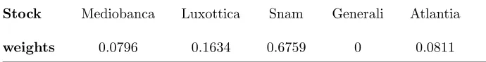
Table 1: Minimum CVaR Portfolio based on ODC

Stock Mediobanca Luxottica Snam Generali Atlantia

weights 0.0796 0.1634 0.6759 0 0.0811

Portfolio and the Minimum CVaR Portfolio using the returns at times 1, . . . , T

of all thep= 24 stocks (Tables 2 and 3). Computations for Markowitz portfolios

have been carried out using the R packagefPortfolio.

The three portfolios (Markowitz minimum variance Portfolio, Minimum CVaR

Portfolio, Minimum CVaR Portfolio based on ODC) exhibit a quite similar

structure, the one based on ODC being the most parsimonious, as it requires

investment on 4 stocks, while the other two results composed by 8 and 6 stocks,

respectively. A barplot of the weights of the stocks in the three portfolios is

displayed in Figure 8.

Finally we check the performance of the three portfolios with an

out-of-sample perspective, in the period from November 1, 2011 to December 20, 2011,

that is at timesT+ 1, . . . , T+ 36. The Minimum CVaR Portfolio based on ODC

tends to outperform the other two (Figure 9).

5.3.2 Strategy B

As pointed out in Section 3.2, portfolios built according to strategy B usually

need to be frequently rebalanced, as they rely on instantaneous clustering

solu-tions. In this case study we decide to update the portfolio composition every 5

days. So, for the out-of-sample period from November 1, 2011 to December 20,

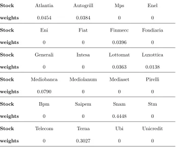
Table 2: Markowitz minimum variance Portfolio

Stock Atlantia Autogrill Mps Enel

weights 0.0454 0.0384 0 0

Stock Eni Fiat Finmecc Fondiaria

weights 0 0 0.0396 0

Stock Generali Intesa Lottomat Luxottica

weights 0 0 0.0363 0.0138

Stock Mediobanca Mediolanum Mediaset Pirelli

weights 0.0790 0 0 0

Stock Bpm Saipem Snam Stm

weights 0 0 0.4448 0

Stock Telecom Terna Ubi Unicredit

Table 3: Minimum CVaR Portfolio

Stock Atlantia Autogrill Mps Enel

weights 0.0750 0 0 0

Stock Eni Fiat Finmecc Fondiaria

weights 0 0 0.0392 0

Stock Generali Intesa Lottomat Luxottica

weights 0 0 0 0.0705

Stock Mediobanca Mediolanum Mediaset Pirelli

weights 0.0884 0 0 0

Stock Bpm Saipem Snam Stm

weights 0 0 0.3913 0

Stock Telecom Terna Ubi Unicredit

ATLANTIA AUTOGRILL MPS ENEL ENI FIAT FINMECC FONDIARIA GENERALI INTESA LOTTOMAT LUXOTTICA MEDIOBANCA MEDIOLANUM MEDIASET PIRELLI BPM SAIPEM SNAM STM TELECOM TERNA UBI UNICREDIT

Minimum CVaR Portfolio based on ODC Minimum CVaR Portfolio

Markowitz minimum variance Portfolio

Weights

0.0 0.1 0.2 0.3 0.4 0.5 0.6

0 5 10 15 20 25 30 35

−20

−15

−10

−5

0

2011: November, 1 − December, 22

Retuns with respect to October

, 31

Markowitz minimum variance Portfolio Minimum CVar Portfolio Minimum CVaR Portfolio based on ODC

Figure 9: Portfolio returns, Strategy A compared with classical portfolios

7),T+ 10 (November 14),T+ 15 (November 21),T+ 20 (November 28),T+ 25

(December 5),T+ 30 (December 12),T+ 35 (December 19). At the end of day

T+hwe estimate the dissimilarity matrix for the following day, ∆T+h+1. In

order to lighten the computational burden, the estimates of the tail dependence

coefficients are computed using parameters estimated up to time T and price

returns up to timeT+i. In other words, we only update the information about

the realized returns, and do not compute new estimates for the parameters of

the involved statistical models. The dissimilarity matrix ∆T+h+1is then used to

cluster thepstocks using the two-step clustering procedure described in Section

3.1. Letkbe the number of clusters and n1, . . . , nk their sizes, we can build a

selecting stocks not belonging to the same cluster. For each of these (n1·. . .·nk)

possible selections, we estimate the weights of the Minimum CVaR Portfolios

using returns at times 1, . . . , T+hand we finally select the solution which

ex-hibits the lowest CVaR value. The corresponding portfolio is then invested for

the following 5 days, i.e. at timesT +h+ 1, . . . , T+h+ 5. At the end of day

T+h+ 5 the procedure is repeated and a new portfolio is built for investing

during the following 5 days. The obtained portfolios are summarized in Table

4. In the short analysed period we do not observe appreciable changes in the

composition of the portfolios, as the dynamic clustering in the out-of-sample

data is fairly stable.

Also in this case, the returns of this investment strategy are compared to the

returns of two competitors: a Markowitz minimum variance Portfolio and the

Minimum CVaR Portfolio built using all thep= 24 stocks and renewed every

5 days (Figure 10). The proposed strategy tends to outperform the other two.

Due to the substantial stability in the portfolios updated every 5 days, the

returns deriving from the two proposed investment strategies, A and B, are

very close each other (Figure 11). So, in this case study, the Minimum CVaR

Portfolio based on ODC outperforms even the competitors (Markowitz minimum

variance and Minimum CVaR) rebalanced every 5 days, which also suffer of

Table 4: Minimum CVaR Portfolios rebalanced every 5 days

Time: T (October 31), k= 4

Stock Mediobanca Luxottica Snam Atlantia

weights 0.0796 0.1634 0.6759 0.0811

Time: T+ 5 (November 7), k= 4

Stock Mediobanca Luxottica Snam Atlantia

weights 0.0398 0.1746 0.7100 0.0756

Time: T+ 10 (November 14), k= 4

Stock Mediobanca Luxottica Snam Atlantia

weights 0.0505 0.2009 0.7056 0.0430

Time: T+ 15 (November 21), k= 4

Stock Mediobanca Luxottica Snam Atlantia

weights 0.0380 0.1977 0.7082 0.0561

Time: T+ 20 (November 28), k= 4

Stock Ubi Luxottica Snam Atlantia

weights 0 0.2187 0.7507 0.0306

Time: T+ 25 (December 5), k= 4

Stock Mediobanca Luxottica Snam Atlantia

weights 0.0417 0.1784 0.7039 0.0760

Time: T+ 30 (December 12), k= 4

Stock Mediobanca Luxottica Snam Atlantia

weights 0.0239 0.1972 0.7032 0.0757

Time: T+ 35 (December 19), k= 4

Stock Mediobanca Luxottica Snam Atlantia

0 5 10 15 20 25 30 35

−20

−15

−10

−5

0

2011: November, 1 − December, 22

Retuns with respect to October, 31

Markowitz minimum variance Portfolio (updated every 5 days) Minimum CVar Portfolio (updated every 5 days) Clustering−based Minimum CVar Portfolio (updated every 5 days)

Figure 10: Portfolio returns, Strategy B compared with classical portfolios

0 5 10 15 20 25 30 35

−20

−15

−10

−5

0

2011: November, 1 − December, 22

Retuns with respect to October, 31

Minimum CVaR portfolio based on ODC

Clustering−based Minimum CVar Portfolio (updated every 5 days)

6

Discussion

In this paper we have proposed two portfolio selection strategies based on a

dynamic clustering of the time series of returns observed for a set of candidate

stocks. The dissimilarity matrix on which the stocks are clustered is derived from

their lower tail dependence coefficients, estimated by means of copula functions

with time-varying parameters. Thanks to this dissimilarity measure based on

lower tail dependence, time series are clustered according to a similar behavior

in event of extremely low returns, so that we propose, as a basic criterion, not

to include in the portfolio stocks belonging to the same cluster. As a portfolio

selection procedure, we propose to optimize the Conditional-Value-at-Risk, as

this is consistent with the approach focused on extreme events.

The main advantages of the proposed method are:

• the time-varying copula functions model the relationship between lower

tail dependence coefficients and the volatility of the market, so as to take

into account contagion phenomenons;

• the diversification of the portfolio is strongly driven by the association

of returns in the lower tail of their joint distribution, and this protects

investments during financial crisis periods;

• the time-varying dissimilarity matrix results in a dynamic clustering

solu-tion which allows us a frequent portfolio rebalancement, if necessary.

A case study with real data from the Italian Stock Market during a financial

classical alternative methods. As future research, a criterion could be developed

to decide which of the two strategies should be used in a given period and to

automatically switch from one to another when it is the case. Furthermore,

the procedure could be refined in order to take into account the upper tail

dependence, which would allow us to take the best from bulls, while protecting

from bears.

References

[1] Davies, D.L., and Bouldin, D. W. (1979), ”A Cluster Separation Measure”.

IEEE Transactions on Pattern Analysis and Machine Intelligence, 1,

224-227.

[2] De Luca, G., and Zuccolotto, P. (2011), ”A Tail Dependence-based

Dissim-ilarity Measure for Financial Time Series Clustering”.Advances in

Classi-fication and Data Analysis, 5, 323-340.

[3] De Luca, G., and Zuccolotto, P. (2012), ”Time Series

Cluster-ing on Lower Tail Dependence”. Proceedings of MAF2012, 2012:

maf2012.unive.it/viewpaper.php?id=101.

[4] Dolniˇcar, S., Leisch, F., Weingessel, A., Buchta, C., and Dimitriadou, E.

A. (1998), ”Comparison of Several Cluster Algorithms on Artifcial Binary

Data Scenarios from Tourism Marketing”.SFB Adaptive Information

Sys-tems and Modeling in Economics and Management Science, Working Paper

[5] Dimitriadou, E., Dolniˇcar, S., and Weingessel, A. (2002), ”An Examination

of Indexes for Determining the Number of Clusters in Binary Data Sets”.

Psychometrika, 67, 137-159.

[6] Friedman, H. P., and Rubin, J. (1967), ”On Some Invariant Criteria for

Grouping Data”.Journal of the American Statistical Association, 62,

1159-1178.

[7] Hartigan, J. A., and Wong, M. A. (1979), ”A K-means Clustering

Algo-rithm”. Applied Statistics, 28, 100-108.

[8] Joe, H. Multivariate Models and Dependence Concept. Chapman & Hall,

New York, 1997.

[9] Krokhmal, P., Palmquist, J., and Uryasev, S. (2002), ”Portfolio

Optimiza-tion with CondiOptimiza-tional Value-at-Risk Objective and Constraints”Journal of

Risk, 4, 43-68.

[10] Nelsen RB.An Introduction to Copulas. Springer-Verlag, New York, 2006.

[11] Rand WM. ”Objective Criteria for the Evaluation of Clustering Methods”.

Journal of the American Statistical Association, 1971; 66:846-850.

[12] Ratkowsky DA, Lance GN. ”A Criterion for Determining the Number of

Groups in a Classifcation”.Australian Computer Journal; 1978; 10:115-117.

[13] Rockafellar RT, Uryasev S. ”Optimization of Conditional Value-at-Risk”.

[14] Scott AJ, Symons MJ. ”Clustering Methods Based on Likelihood Ratio

Criteria”.Biometrics, 1971; 27:387-397.

[15] Sokal RR, Michener CD. ”A Statistical Method for Evaluating Systematic