Forecasting Realized Volatility of Russian stocks using Google Trends and Implied Volatility

Munich Personal RePEc Archive

Forecasting Realized Volatility of Russian

stocks using Google Trends and Implied

Volatility

Bazhenov, Timofey and Fantazzini, Dean

April 2019

Online at

https://mpra.ub.uni-muenchen.de/93544/

Forecasting Realized Volatility of Russian stocks

using Google Trends and Implied Volatility

Timofey Bazhenov

Dean Fantazzini

Abstract

This work proposes to forecast the Realized Volatility (RV) and the Value-at-Risk (VaR) of the most liquid Russian stocks using GARCH, ARFIMA and HAR mod-els, including both the implied volatility computed from options prices and Google Trends data. The in-sample analysis showed that only the implied volatility had a significant eff_{ect on the realized volatility across most stocks and estimated}

mod-els, whereas Google Trends did not have any significant eff_{ect. The out-of-sample}

analysis highlighted that models including the implied volatility improved their fore-casting performances, whereas models including internet search activity worsened their performances in several cases. Moreover, simple HAR and ARFIMA models without additional regressors often reported the best forecasts for the daily realized volatility and for the daily Value-at-Risk at the 1% probability level, thus showing that effi_{ciency gains more than compensate any possible model misspecifications and}

parameters biases. Our empirical evidence shows that, in the case of Russian stocks, Google Trends does not capture any additional information already included in the implied volatility.

Keywords: Forecasting, Realized Volatility, Value-at-Risk, Implied Volatility, Google Trends, GARCH, ARFIMA, HAR.

JEL classification: C22, C51, C53, G17, G32.

Russian Journal of Industrial Economics

, forthcoming

∗_{Higher School of Economics, Moscow (Russia)}

1

Introduction

Volatility forecasting is of cardinal importance in several applications, from derivatives

pricing to portfolio and risk management, see [1] for a large survey. Recent literature

suggested the idea to consider the investors’ behavior measured by the internet search

volumes as a factor influencing the assets volatility, see for example [2] and references

therein for more details. The investors’ interest was originally quantified using some

proxy measures like news or turnover. However, [3] showed that these proxies do not

im-prove the forecasting of volatility. Instead, recent works by [4] and [5] reported empirical

evidence showing that online search volumes are a good predictor of volatility. This

pa-per aims to estimate the predictive power of online search activity (as proxied by Google

Trends data) and implied volatility (computed from option prices) for forecasting the

re-alized volatility of several Russian stocks. In this regard, the implied volatility measures

the investors’ sentiment about the future performance of an asset, see the survey of [6]

and references therein for more details. These two measures of investors’ attention and

expectations are then used to forecast the realized volatility of Russian stocks by using

three competing models: the Heterogeneous Auto-Regressive (HAR) model by [7], the

AutoRegressive Fractional (ARFIMA) model by [8], and a simple GARCH(1,1) model.

The forecasting performances of these models are compared using the usual forecasting

diagnostics, such as the mean squared error (MSE), and the Model Confidence Set by [9].

The models volatility forecasts are also employed to compute the Value-at-Risk for each

asset to measure their market risk. The first contribution of this paper is an evaluation of

the contribution of both online search intensity and options-based implied volatility to the

modelling of realized volatility for Russian stocks. To our knowledge, this analysis has

not been done elsewhere. The second contribution is an out-of-sample forecasting

Google data and implied volatility. The third contribution of the paper is a backtesting

exercise to measure the accuracy of Value-at-Risk forecasts. The rest of this paper is

or-ganized as follows. Section 2 briefly reviews the literature devoted to Google Trends and

implied volatility, while the methods proposed for forecasting the realized volatility and

the VaR are discussed in Section 3. The empirical results are reported in Section 4, while

Section 5 briefly concludes.

2

Literature review

There is an increasing body of the financial literature which examines how online searches

aff_{ect asset pricing and volatility modelling. We review some of these works which are}

closely related to our research topic. [5] considered the top-30 stocks (in terms of volume)

traded on the NYSE and used the search volumes involving the name of the company as

a proxy of demand for firm-specific information. They found that such demand for

in-formation contains potentially useful signals because it is strongly related to the stock

trading volumes and the historical volatility. [2] evaluated the marginal predictive power

of Google trends to forecast the Crude Oil Volatility index by using HAR models and

sev-eral macro-finance variables. More specifically, they employed the standard HAR model,

the HAR model including macroeconomic variables, the HAR model with online search

volumes and the HAR model including both search volumes and macroeconomic

vari-ables. They found that the amount of online searches has a positive relationship with the

oil volatility index. Moreover, this association remains significant even when

macroe-conomic variables are included in the model, thus highlighting that Google data capture

some extra information. [9] examined the relationship between investors’ interest and the

foreign exchange market volatility. They showed a strong connection between the changes

variables. [10] evaluated the role of the online search activity for forecasting realized

volatility of financial markets and commodity markets using models that also include

market-based variables. They found that Google search data play a minor role in

pre-dicting the realized volatility once implied volatility is included in the set of regressors.

Therefore, they suggested that there might exist a common component between implied

volatility and Internet search activity: in this regard, they found that most of the predictive

information about realized volatility contained in Google Trends data is also included in

implied volatility, whereas implied volatility has additional predictive content that is not

captured by Google data.

3

Methodology

3.1

Measures of volatility

3.1.1 Realized Variance

Real volatility is not observable, so a proxy is needed for its observation. The realized

variance (RV) is probably the best proxy available: [11] showed that the RV is a consistent

estimator of the actual variance, while [12] compared more than 400 estimators of price

variation and they came to the conclusion that it is diffi_{cult to significantly outperform}

the 5-minute RV estimator. For this reason, we used this estimator in this work. Suppose

that on the trading dayt, Mprices were observed at times t0,t1,...,tM. Ifptjstands for the

logarithmic price at timetj, then the log-returnrtj for thej-th interval of day tis defined

as,rtj=ptj−ptj-1. The formula for the realized variance is thus given by:

RVt = M X

j=₁

Over a time horizon ofk days, the realized variance is computed asRVt:t+k = Pki=₁RVt+_i

, under the convention that RVt =RVt−1:t. Horizons of 1 (daily), 5 (weekly) and 22

(monthly) days were considered.

3.1.2 Implied volatility

The implied volatility (IV) of an option contract is the value of the volatility of the

un-derlying asset which makes the theoretical value of the option -computed using an option

pricing model like the Black–Scholes model- equal to the current market price of the

op-tion, see [6] and [13] for details. The implied volatility reflects the investors’ expectations

and sentiments and, if the assumptions of the Black-Scholes model hold, it is an effi_cient

predictor of the actual volatility of the underlying asset. Assuming that all the other

pa-rameters of the Black-Scholes model are available (that is, the stock and strike prices, the

risk-free rate, the time to expiration and the market price of the option), then the IV can

be computed using nonlinear optimization methods, like the Newton-Raphson algorithm,

see [14] and references therein.

3.2

Data

Intraday data sampled every 5 minutes for the most liquid Russian stocks (Sberbank

-SBER, Rosneft -ROSN, Yandex-YNDX, Gazprom- GAZP, where the four-letter

abbrevi-ations are the stocks tickers) were downloaded from the websitefinam.ru. Option prices

from the Moscow exchange were used to compute the implied volatility for each asset.

The dataset covered the period from January 2016 till April 2018.

Google Trends computes how many searches were made for a keyword or a topic on

Google over a specific period of time and a specific region. This amount is then divided

series is divided by its highest value and multiplied by 100, so that all data are normalized

between 0 and 100. The tickers of the Russian stocks described above were used as a

search keyword used by investors to get information for a particular company. All search

volumes were downloaded from the Google Trends website using the R packagegtrendsR.

These data were then merged with the search volumes for the queries in Russian looking

for a specific stock price, for example “Sberbank share price”.

3.3

Models

3.3.1 HAR model

The Heterogeneous Auto-Regressive model for the realized volatility was first proposed

by [7] and it allows to reproduce several stylized facts of assets’ volatility. The HAR

model is specified as follows,

RVt+₁=β₀ +β_DRV_t +β_WRV_t−5:t +β_MRV_t−22:t +ε_t+₁

whereD,W and M stand for daily, weekly and monthly values of the realized volatility,

respectively. The main novelty of our work is the inclusion of the implied volatility and

Google Trends as additional regressors to forecast the realized volatility of Russian stocks:

RVt+₁=β₀+β_DRV_t+β_WRV_t−5:t+β_MRV_t−22:t+γGT_t+αIV_t +ε_t+₁

3.3.2 ARFIMA model

[8] proposed the Auto-Regressive Fractional Integrated Moving Average (ARFIMA) model

to forecast the realized volatility, and it has been one of the best models ever since. The

ARFIMA(p,d,q) model is given by:

Φ_(L)(1−L)d_(RV

whereLis the lag operator, Φ _(L)= _{1 − ϕ1L −... − ϕpL}p_, Θ_(L) = ₁+ _{θ 1L}+ _... + _θ

qLqand (1−L)dis the fractional differencing operator defined by:

(1−L)d =

∞

X

k=₀

Γ_(k−d)Lk Γ_(−d)Γ_(k+₁₎

whereΓ_{(•) is the gamma function. Similarly to the HAR model, we also considered the}

case where the implied volatility and Google Trends are added as (external) regressors, so

the model becomes:

Φ_(L)(1−L)d_(RVt+₁−µ)=γGT_t +αIV_t+ Θ(L)ε_t+₁

[15] proposed an algorithm for the automatic selection of the optimal ARFIMA model,

which is implemented in the R packagesforecastandrugarch.

3.3.3 GARCH model

The Generalized Auto-Regressive Conditional Heteroscedasticity (GARCH) models are

extensively used in empirical finance, thanks to their good forecasting performances:

for example, [16] compared more than 330 volatility models and they found no

evi-dence that a GARCH(1,1) can be outperformed by more sophisticated models. A general

GARCH(p,q) model for the conditional variance equation can be specified as follows:

σ2_t =_α0+ q X

i=₁

αiε2t−i+ q X

j=₁

βjσ2t−j

whereσ2_t is the conditional variance at timet. A simple GARCH (1,1) model with

stan-dardized errors following a Student’s t-distribution was employed in this work. Similarly

to the HAR and ARFIMA models, we also considered a GARCH specification including

3.4

Forecast Comparison

3.4.1 Variance forecasts

We divided the data into a training dataset used to estimate the models (the first 67% of

the sample), and a test dataset to evaluate the models’ performances. We computed the

1-day-ahead volatility forecasts of our competing models and we compared them using the

mean square error (MSE). We also employed the Model Confidence Set proposed by [17],

which can select the best performing model(s) at a predefined confidence level. Given a

specific loss function, in our case the squared loss, Lossi,t =

c

RVi,t−RVi,t

2

, where RV

and RVc stand for the observed and forecasted level of the realized volatility, then the

diff_{erence between the losses of models i and j at time t can be computed as follows:}

di,j,t = Lossi,t −Lossj,t. The hypothesis of equal predictive ability suggested by [17] can

be formulated as:

H0,M : E(di,j,t)=0,for all i,j∈M,

whereMis the set of forecasting models. First, the following t-statistics are calculated

ti j =

¯

di j c

vard¯i j

f or i, j∈M

where ¯di j = T−1PTt=₁di j,t andvarc

di j

is a bootstrapped estimate of vard¯i j

. Then, this

test statistic is computed: TR,M = maxi∈M|ti j|. This statistic has a non-standard

distribu-tion, so the distribution under the null hypothesis is computed via bootstrap. If the null

hypothesis is rejected, one model is eliminated from the analysis by using the following

rule:

eRM = argmaxi (

sup

j∈M

¯

di j c

The number of models is diminished by 1 and the testing procedure starts from the

be-ginning. For volatility forecasts, the previous MSE loss was used, whereas the symmetric

quantile loss function proposed by [18] was used for the VaR forecasts (more details in

the next section).

3.4.2 Value-at-Risk forecasts

The Value-at-Risk is the potential market loss of a financial asset over a time horizonh

with probability levelα. The VaR is a widely used measure of market risk in the

finan-cial sector, and we refer to [19] for a large survey of realized volatility models and VaR

methods.

In this work, we consideredh=_{1 and the probability levelsα}=_{5% andα}=_{1%. In the}

case of HAR and ARFIMA models, the 1-day ahead VaR can be computed as follows:

VaRt+₁,α =Φ−1α

q c

RVt+₁

where_Φ−1

α is the inverse function of a standard normal distribution function at the

prob-ability levelα, whileRVct+₁ is the 1-day-ahead forecast for the realized volatility. In the

case of GARCH models with student’s t errors, the 1-day ahead VaR can be computed as

follows:

VaRt+₁,α= µˆt+₁+t−1_α,ν

q

ˆ σ2_t+₁

where ˆµt+₁is the 1-day-ahead forecast of the conditional mean, ˆσ2_t+1is the 1-day-ahead

forecast of the conditional variance, whilet−1

α,ν is the inverse function of the Student’s t

distribution withνdegrees of freedom at the probability levelα.

To compare the forecasting performance of the diff_{erent VaR models, the forecasted}

values of the VaR are compared to the actual returns for each day, and the number of

the number of violations are counted): a “perfect VaR model” would deliver a number

of violations which is not predictable and exactly equal to α%. We can test the null

hypothesis that the fraction of actual violationsπfor a forecasting model is significantly

diff_{erent fromαusing the unconditional coverage test by [20]. The joint null hypothesis}

that the VaR violations are independent and the average number of violations is correct can

be tested using the conditional coverage test by [21]: diff_{erently from the unconditional}

coverage test, the Christoff_{ersen’s test also considers the dependence of violations for}

consecutive days. Finally, noting that financial regulators are also concerned with the

magnitude of the VaR violations, we computed the asymmetric quantile loss (QL) function

proposed by [18]:

QL_t+₁,α =(α−It+₁(α))(y_t+₁−VaR_t+_1,α)

whereIt+₁(α)=1 ify_t+₁ <VaR_t+_1,αand zero otherwise.

3.5

In-sample analysis

For sake of space and interest, we report in Tables 1-4 the parameters estimates for the

HAR model under diff_{erent specifications -with and without the implied volatility and}

Google Trends-, while Table 5 summarizes the parameters estimates across diff_erent

mod-els by showing only the estimated parameters of the implied volatility and Google Trends

Table 1: Summary of HAR models for SBERBANK

Dependent variable: RVt+1

RVt −6.16e-02 −6.57e-02 −6.54e-02 −6.10e-02

(4.43e-02) (4.40e-02) (4.40e-02) (4.43e-02)

RVweekly 5.13e-03∗ ∗ ∗ _5.80e-03∗ ∗ ∗ _5.86e-03∗ ∗ ∗ _5.26e-03∗ ∗ ∗

(1.53e-03) (1.53e-03) (1.54e-03) (1.54e-03)

RVmonthly −2.52e-03 −9.25e-03∗ ∗ _−9.45e-03∗ ∗ _−3.12e-03

(4.12e-03) (4.66e-03) (4.71e-03) (4.22e-03)

IVt 2.08e-07∗ ∗ ∗ 2.05e-07∗ ∗ ∗

(6.92e-08) (6.98e-08)

GTt −3.26e-09 −6.63e-09

(9.79e-09) (9.80e-09)

Constant 3.10e-06∗ ∗ ∗ _{−2.19e-06 −1.91e-06 3.52e-06}∗ ∗ ∗

(8.783e-07) (1.96e-06) (2.14e-06) (1.08e-06)

Note:∗_p<0.1;∗ ∗_p<0.05;∗ ∗ ∗_p<0.01

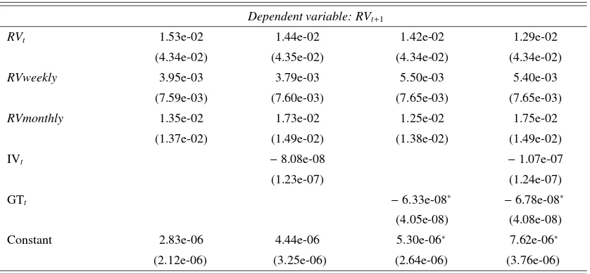
Table 2: Summary of HAR models for GAZPROM

Dependent variable: RVt+1

RVt 1.53e-02 1.44e-02 1.42e-02 1.29e-02

(4.34e-02) (4.35e-02) (4.34e-02) (4.34e-02)

RVweekly 3.95e-03 3.79e-03 5.50e-03 5.40e-03

(7.59e-03) (7.60e-03) (7.65e-03) (7.65e-03)

RVmonthly 1.35e-02 1.73e-02 1.25e-02 1.75e-02

(1.37e-02) (1.49e-02) (1.38e-02) (1.49e-02)

IVt −8.08e-08 −1.07e-07

(1.23e-07) (1.24e-07)

GTt −6.33e-08∗ −6.78e-08∗

(4.05e-08) (4.08e-08)

Constant 2.83e-06 4.44e-06 5.30e-06∗ _7.62e-06∗

(2.12e-06) (3.25e-06) (2.64e-06) (3.76e-06)

Table 3: Summary of HAR models for YANDEX

Dependent variable: RVt+1

RVt 1.97e-02 1.63e-02 1.97e-02 1.63e-02

(4.33e-02) (4.33e-02) (4.34e-02) (4.34e-02)

RVweekly −8.02e-04 −1.12e-03 −8.72e-04 −1.19e-03

(1.23e-03) (1.24e-03) (1.28e-03) (1.30e-03)

RVmonthly 8.89e-03∗ ∗ ∗ _8.72e-03∗ ∗ ∗ _8.94e-03∗ ∗ ∗ _8.78e-03∗ ∗ ∗

(2.37e-03) (2.37e-03) (2.39e-03) (2.39e-03)

IVt 9.49e-08∗ 9.49e-08∗

(5.73e-08) (5.73e-08)

GTt 5.79e-09 5.75e-09

(2.96e-08) (2.96e-08)

Constant −8.00e-07 −4.30-06∗ _{−8.47e-07 −4.34e-06}∗

(1.20e-06) (2.43e-06) (1.22e-06) (2.44e-06)

Note:∗_p<0.1;∗ ∗_p<0.05;∗ ∗ ∗_p<0.01

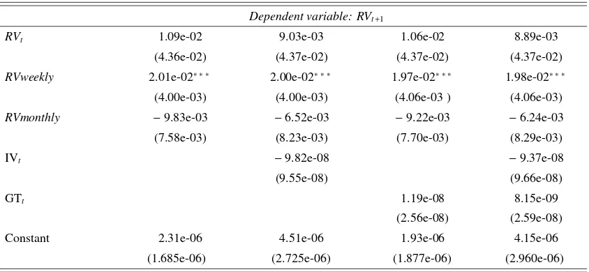
Table 4: Summary of HAR models for ROSNEFT

Dependent variable: RVt+1

RVt 1.09e-02 9.03e-03 1.06e-02 8.89e-03

(4.36e-02) (4.37e-02) (4.37e-02) (4.37e-02)

RVweekly 2.01e-02∗ ∗ ∗ _2.00e-02∗ ∗ ∗ _1.97e-02∗ ∗ ∗ _1.98e-02∗ ∗ ∗

(4.00e-03) (4.00e-03) (4.06e-03 ) (4.06e-03)

RVmonthly −9.83e-03 −6.52e-03 −9.22e-03 −6.24e-03

(7.58e-03) (8.23e-03) (7.70e-03) (8.29e-03)

IVt −9.82e-08 −9.37e-08

(9.55e-08) (9.66e-08)

GTt 1.19e-08 8.15e-09

(2.56e-08) (2.59e-08)

Constant 2.31e-06 4.51e-06 1.93e-06 4.15e-06

(1.685e-06) (2.725e-06) (1.877e-06) (2.960e-06)

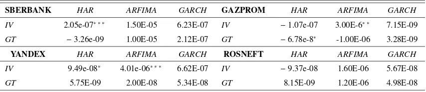
Table 5: Summary of the estimated parameters of the implied volatility and Google Trends across diff_erent

models

SBERBANK HAR ARFIMA GARCH GAZPROM HAR ARFIMA GARCH

IV 2.05e-07∗ ∗ ∗

1.50E-05 6.23E-07 IV −1.07e-07 3.00E-6∗ ∗

7.15E-09

GT −3.26e-09 1.00E-05 2.12E-07 GT −6.78e-8∗

-1.00E-06 3.28E-09

YANDEX HAR ARFIMA GARCH ROSNEFT HAR ARFIMA GARCH

IV 9.49e-08∗ _4.01e-06∗ ∗ ∗ _{6.62E-07 IV −9.37e-08 1.60E-06 5.67E-08}

GT 5.75E-09 2.00E-08 5.34E-08 GT 8.15E-09 1.20E-06 4.98E-08

Note:∗_p

<0.1;∗ ∗_p

<0.05;∗ ∗ ∗_p

<0.01

In general, only the implied volatility has a significant eff_{ect on the realized volatility}

across most stocks and estimated models. Instead, Google Trends does not seem to have

any appreciable eff_{ect on the realized volatility, thus confirming similar evidence reported}

by [10].

3.6

Out-of-sample analysis

3.6.1 Variance forecasts

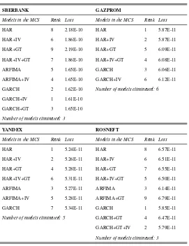
The models included in the Model Confidence Set (MCS) at the 10% confidence level and

Table 6: Models included in the MCS at the 10% confidence level and associated mean squared loss

SBERBANK GAZPROM

Models in the MCS Rank Loss Models in the MCS Rank Loss

HAR 8 2.18E-10 HAR 1 5.87E-11

HAR+IV 6 1.86E-10 HAR+IV 2 5.87E-11

HAR+GT 9 2.19E-10 HAR+GT 5 6.09E-11

HAR+IV+GT 7 1.86E-10 HAR+IV+GT 4 6.08E-11

ARFIMA 5 1.65E-10 GARCH 3 6.06E-11

ARFIMA+IV 4 1.65E-10 GARCH+IV 6 6.12E-11

GARCH 2 1.62E-10 Number of models eliminated: 6

GARCH+IV 1 1.61E-10

GARCH+GT 3 1.65E-10

Number of models eliminated: 3

YANDEX ROSNEFT

Models in the MCS Rank Loss Models in the MCS Rank Loss

HAR 1 5.24E-11 HAR 8 6.57E-11

HAR+IV 2 5.26E-11 HAR+IV 6 6.51E-11

HAR+GT 4 5.28E-11 HAR+GT 7 6.55E-11

HAR+IV+GT 6 5.31E-11 HAR+IV+GT 5 6.50E-11

ARFIMA 3 5.27E-11 ARFIMA 3 6.14E-11

ARFIMA+IV 5 5.28E-11 ARFIMA+GT 9 6.79E-11

GARCH 7 5.34E-11 GARCH 1 5.85E-11

Number of models eliminated: 5 GARCH+GT 4 6.47E-11

GARCH+GT+IV 2 5.79E-11

Number of models eliminated: 3

The models including the implied volatility tend to have smaller MSE compared to

other models, but these diff_{erences are not statistically significant and several}

compet-ing models are also included into the MCS. Interestcompet-ingly, the simple HAR and GARCH

models without additional regressors have the smallest MSE for 3 stocks out of 4, thus

showing that effi_{ciency gains more than compensate any possible model misspecifications}

3.6.2 Value-at-Risk forecasts

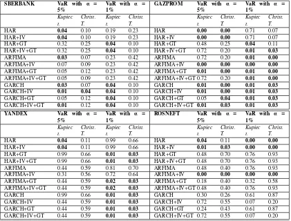
The p-values of the Kupiec and Christoff_{ersen’s tests are reported in Table 7, while the}

models included in the Model Confidence Set (MCS) at the 10% confidence level and

their associated asymmetric quantile loss are reported in Table 8.

Table 7: Kupiec tests p-values and Christoff_{ersen’s tests p-values. P-values smaller than 0.05 are in bold font.}

SBERBANK VaR with α ₌ 5%

VaR with α ₌ 1%

GAZPROM VaR with α ₌ 5%

VaR with α ₌ 1% Kupiec t. Christ. T. Kupiec t. Christ. T. Kupiec t. Christ. T. Kupiec t. Christ. T.

HAR 0.04 0.10 0.19 0.23 HAR 0.00 0.00 0.71 0.07 HAR+_{IV 0.04 0.10 0.19 0.23 HAR}+_{IV 0.00 0.00 0.71 0.07}

HAR+_{GT 0.32 0.25 0.04 0.10 HAR}+_{GT 0.48 0.25 0.04 0.11}

HAR+_IV+_{GT 0.32 0.25 0.04 0.10 HAR}+_IV+_{GT 0.72 0.20 0.01 0.03}

ARFIMA 0.03 0.07 0.23 0.42 ARFIMA 0.72 0.20 0.01 0.00

ARFIMA+_{IV 0.07 0.09 0.23 0.42 ARFIMA}+_{IV 0.00 0.00 0.00 0.00}

ARFIMA+_{GT 0.05 0.12 0.23 0.42 ARFIMA}+_{GT 0.01 0.00 0.01 0.00}

ARFIMA+_IV+_{GT 0.05 0.09 0.23 0.42 ARFIMA}+_IV+_{GT 0.72 0.20 0.01 0.00}

GARCH 0.03 0.07 0.04 0.10 GARCH 0.01 0.00 0.01 0.03

GARCH+_{IV 0.01 0.04 0.04 0.10 GARCH}+_{IV 0.01 0.00 0.01 0.03}

GARCH+_{GT 0.05 0.12 0.04 0.10 GARCH}+_{GT 0.05 0.04 0.01 0.03}

GARCH+_IV+_{GT 0.01 0.12 0.04 0.10 GARCH}+_IV+_{GT 0.01 0.03 0.01 0.03}

YANDEX VaR with α ₌ 5%

VaR with α ₌ 1%

ROSNEFT VaR with α ₌ 5%

VaR with α ₌ 1% Kupiec t. Christ. T. Kupiec t. Christ. T. Kupiec t. Christ. T. Kupiec t. Christ. T.

HAR 0.04 0.11 0.99 0.66 HAR 0.04 0.11 0.00 0.00

HAR+_{IV 0.04 0.11 0.99 0.66 HAR}+_{IV 0.01 0.03 0.00 0.00}

HAR+_{GT 0.99 0.66 0.01 0.03 HAR}+_{GT 0.48 0.70 0.76 0.93}

HAR+_IV+_{GT 0.99 0.66 0.01 0.03 HAR}+_IV+_{GT 0.48 0.70 0.76 0.93}

ARFIMA 0.44 0.59 0.81 0.70 ARFIMA 0.48 0.40 0.76 0.93 ARFIMA+_{IV 0.31 0.56 0.72 0.64 ARFIMA}+_{IV 0.00 0.00 0.00 0.00}

ARFIMA+_{GT 0.44 0.59 0.02 0.03 ARFIMA}+_{GT 0.18 0.40 0.32 0.58}

ARFIMA+_IV+_{GT 0.44 0.59 0.02 0.03 ARFIMA}+_IV+_{GT 0.48 0.40 0.76 0.93}

GARCH 0.99 0.66 0.01 0.03 GARCH 0.30 0.26 0.61 0.87 GARCH+_{IV 0.44 0.59 0.01 0.03 GARCH}+_{IV 0.72 0.55 0.07 0.20}

GARCH+_{GT 0.44 0.59 0.01 0.03 GARCH}+_{GT 0.24 0.43 0.61 0.87}

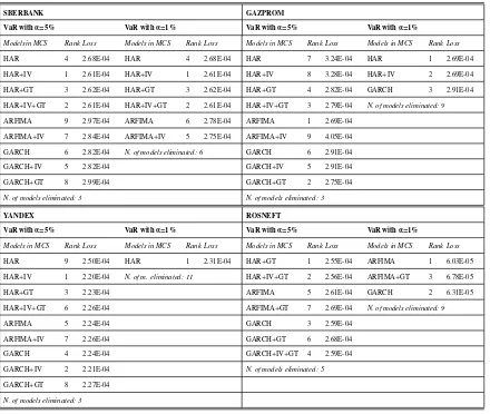
Table 8: Models included in the MCS at the 10% confidence level and associated asymmetric quantile loss.

SBERBANK GAZPROM

VaR withα₌5% VaR withα₌1% VaR withα₌5% VaR withα₌1%

Modelsin MCS Rank Loss Models in MCS Rank Loss Models in MCS Rank Loss Models in MCS Rank Loss

HAR 4 2.68E-04 HAR 4 2.68E-04 HAR 7 3.24E-04 HAR 1 2.69E-04

HAR+IV 1 2.61E-04 HAR+IV 1 2.61E-04 HAR+IV 8 3.28E-04 HAR+IV 2 2.69E-04

HAR+GT 3 2.62E-04 HAR+GT 3 2.62E-04 HAR+GT 4 2.82E-04 GARCH 3 2.91E-04

HAR+IV+GT 2 2.61E-04 HAR+IV+GT 2 2.61E-04 HAR+IV+GT 3 2.79E-04 N. of models eliminated: 9

ARFIMA 9 2.97E-04 ARFIMA 6 2.78E-04 ARFIMA 1 2.69E-04

ARFIMA+IV 7 2.84E-04 ARFIMA+IV 5 2.75E-04 ARFIMA+IV 9 4.05E-04

GARCH 6 2.82E-04 N. of models eliminated: 6 GARCH 6 2.91E-04

GARCH+IV 5 2.82E-04 GARCH+IV 5 2.91E-04

GARCH+GT 8 2.99E-04 GARCH+GT 2 2.75E-04

N. of models eliminated: 3 N. of models eliminated: 3

YANDEX ROSNEFT

VaR withα₌5% VaR withα₌1% VaR withα₌5% VaR withα₌1%

Models in MCS Rank Loss Models in MCS Rank Loss Models in MCS Rank Loss Models in MCS Rank Loss

HAR 9 2.50E-04 HAR 1 2.31E-04 HAR+GT 1 2.55E-04 ARFIMA 1 6.03E-05

HAR+IV 1 2.20E-04 N. of m. eliminated: 11 HAR+IV+GT 2 2.56E-04 ARFIMA+GT 3 6.78E-05

HAR+GT 3 2.23E-04 ARFIMA 5 2.61E-04 GARCH 2 6.31E-05

HAR+IV+GT 6 2.26E-04 ARFIMA+GT 7 2.69E-04 N. of models eliminated: 9

ARFIMA 5 2.24E-04 GARCH 3 2.59E-04

ARFIMA+IV 7 2.26E-04 GARCH+GT 6 2.68E-04

GARCH 4 2.24E-04 GARCH+IV+GT 4 2.59E-04

GARCH+IV 2 2.21E-04 N. of models eliminated: 5

GARCH+GT 8 2.27E-04

N. of models eliminated: 3

These tables show that ARFIMA and HAR models without additional regressors tend

to be the best compromise for precise VaR forecasts, particularly at the 1% level, which

is the most important quantile for regulatory purposes. The HAR model with the implied

volatility showed in several cases the lowest asymmetric quantile losses, thus confirming

the previous in-sample analysis. However, the diff_{erences with the other models were}

rather small and not statistically significant. Moreover, for two stocks (Yandex and

Ros-neft) the models with the implied volatility were excluded from the MCS for the VaR

bet-ter choice when out-of-sample forecasting is the main concern, thanks to more effi_cient

estimates in comparison to more complex specifications.

4

Conclusions

Three volatility forecasting models and several diff_{erent specifications, including also the}

implied volatility computed from option prices and Google Trends data, were used to

model and forecast the realized volatility and the VaR of four Russian stocks.

The in-sample analysis showed that only the implied volatility had a significant

ef-fect on the realized volatility across most stocks and estimated models, whereas Google

Trends did not have any significant eff_{ect on the realized volatility. The out-of-sample}

analysis highlighted that the models including the implied volatility had smaller MSE

compared to several competing models, but these diff_{erences were not statistically}

sig-nificant. Moreover, the simple HAR and GARCH models without additional regressors

showed the smallest MSE for three stocks out of four, thus showing that effi_{ciency gains}

more than compensate any possible model misspecifications and parameters biases. A

similar result was also found after performing a backtesting analysis with daily VaR

fore-casts, where ARFIMA and HAR models without additional regressors had the best results

in several cases (particularly at the 1% probability level), whereas the HAR model with

implied volatility displayed good results when forecasting the VaR at the 5% probability

level. Therefore, these findings revealed that Google Trends data did not improve the

forecasting performances of the models when a market-based predictor like the implied

volatility was included, thus confirming similar results reported by [10].

How to explain these results? One possible explanation was proposed by [10], who

put forward the idea that the informational content included in the internet search activity

as a surprise, if we consider that implied volatility is a forward-looking measure mainly

based on the expectations of institutional investors and market makers who have access

to premium and insider information, while Google Trends data are mainly based on the

expectations of small investors and un-informed traders. A second simpler explanation

is that Yandex is the main search engine in Russia with a market share close to 56% in

2018 (all platforms), while Google is second with a market share close to 42%, so that

Google Trends may not be the best proxy for Russian investors’ interest and behavior.

More research is definitely needed in this regard, and this issue is left as an avenue of

References

[1] Bauwens, L., Hafner, C. M., and Laurent, S. (2012).Handbook of volatility models and their

appli-cations (Vol. 3). John Wiley and Sons.

[2] Campos, I., Cortazar, G., and Reyes, T. (2017). Modeling and predicting oil VIX: Internet search

volume versus traditional variables.Energy Economics, 66, 194-204.

[3] Donaldson, R. G., and Kamstra, M. J. (2005). Volatility forecasts, trading volume, and the arch versus

option-implied volatility trade-off_{.Journal of Financial Research, 28(4), 519-538.}

[4] Andrei, D., and Hasler, M. (2014). Investor attention and stock market volatility. The Review of

Financial Studies, 28(1), 33-72.

[5] Vlastakis N. and R. N. Markellos. (2012) Information demand and stock market volatility.Journal of

Banking and Finance, 1808–1821.

[6] Mayhew, S. (1995). Implied volatility.Financial Analysts Journal, 51(4), 8-20.

[7] Corsi, F. (2009). A simple approximate long-memory model of realized volatility.Journal of

Finan-cial Econometrics, 174-196.

[8] Andersen, T. G., Bollerslev, T., Diebold, F. X., Labys, P. (2003). Modeling and forecasting realized

volatility.Econometrica, 71(2), 579-625.

[9] Goddard, J., Kita, A., and Wang, Q. (2015). Investor attention and FX market volatility.Journal of

International Financial Markets, Institutions and Money, 38, 79-96.

[10] Basistha, A., Kurov, A., and Wolfe, M. (2018). Volatility Forecasting: The Role of Internet Search

Activity and Implied Volatility, West Virginia University working paper

[11] Barndorff_{-Nielsen, O. E., and Shephard, N. (2002). Econometric analysis of realized volatility and}

its use in estimating stochastic volatility models.Journal of the Royal Statistical Society: Series B

(Statistical Methodology), 64(2), 253-280.

[12] Liu, L. Y., Patton, A. J., and Sheppard, K. (2015). Does anything beat 5-minute RV? A comparison

of realized measures across multiple asset classes.Journal of Econometrics, 187(1), 293-311.

[13] Hull, J. C. (2016).Options, futures and other derivatives. Pearson.

[14] Fengler, M. R. (2006). Semiparametric modeling of implied volatility. Springer Science & Business

[15] Hyndman, R. J., and Khandakar, Y. (2008). Automatic Time Series Forecasting: the forecast Package

for R.Journal of Statistical Software, 27(3).

[16] Hansen, P. R., and Lunde, A. (2005). A forecast comparison of volatility models: does anything beat

a GARCH (1, 1)?.Journal of applied econometrics, 20(7), 873-889.

[17] Hansen, P. R., Lunde, A., & Nason, J. M. (2011). The model confidence set. Econometrica, 79(2),

453-497.

[18] Gonz´alez-Rivera, G., Lee, T. H., and Mishra, S. (2004). Forecasting volatility: A reality check based

on option pricing, utility function, value-at-risk, and predictive likelihood.International Journal of

forecasting, 20(4), 629-645.

[19] Louzis, D. P., Xanthopoulos-Sisinis, S., and Refenes, A. P. (2014). Realized volatility models and

alternative Value-at-Risk prediction strategies.Economic Modelling, 40, 101-116.

[20] Kupiec, P. H. (1995). Techniques for Verifying the Accuracy of Risk Measurement Models. The

Journal of Derivatives, 3(2), 73-84.

[21] Christoff_{ersen, P. F. (1998). Evaluating interval forecasts.International economic review, 39,}